以適應性模糊類神經網路為基礎之縱向車隊強健控制

全文

(1)國立交通大學電機與控制工程學系. 碩士論文. 以適應性模糊類神經網路為基礎之縱向車隊強健控制. Robust Longitudinal Control of a Platoon of Vehicles Based on Adaptive Fuzzy Neural Approach. 研究生 : 范詠建指導教授 : 張隆國博士李祖添博士. 中華民國九十三年七月.

(2) 以適應性模糊類神經網路為基礎之縱向車隊強健控制 Robust Longitudinal Control of a Platoon of Vehicles Based on Adaptive Fuzzy Neural Approach. 學生：范詠建指導教授：張隆國博士李祖添博士. Student：Yung-Chien Fan Advisors：Lon-Kou Chang Tsu-Tian Lee. 國立交通大學電機與控制工程學系碩士論文. A Thesis Submitted to Institute of Electrical and Control Engineering College of Electrical Engineering and Computer Science National Chiao Tung University in Partial Fulfillment of the Requirements for the Degree of Master in Electrical and Control Engineering July 2004 Hsinchu, Taiwan, Republic of China. 中華民國九十三年七月.

(3) 以適應性模糊類神經網路為基礎之縱向車隊強健控制. 學生：范詠建. 指導教授：張隆國博士李祖添博士. 國立交通大學電機與控制工程學系. 摘要在本文中，我們提出以三種不同的縱向車隊控制器，包括模糊控制器，滑動模式控制器，以及以滑動模式觀測器為基礎的滑動模式控制器，並搭配非直接適應性模糊類神經網路近似器及 H ∞ 概念來滿足系統的強健性及表現。對於一列直線行進的車隊，已知隨著前車動態的變化，譬如由低速前進到高速前進，車隊中車輛間的相對距離也將隨之變動，此一車距的改變將被用來改變車隊中後方車子的行進行為。我們的控制策略是施加合理的油門控制力迫使車隊中每部車子之間相對於前方車輛保持適當的安全距離，並以舒適的加減速追隨前方的車子的行進行為。在此假設在車輛行進的過程中，車間相對位置是可量測的。在縱向車隊行進控制上，模糊控制器可呈現良好的控制效果，而滑動模式控制器提供了更穩定且可信賴的控制效果。在引入模糊類神經網路近似器及 H ∞ 概念後維持了系統的強健性及改善了系統控制輸入的切跳現象。為了更符合真實車隊系統的效益，我們假設僅能量測到車間的相對距離。在此限制下，以滑動模式觀測器為基礎的滑動模式控制器亦保證對前車位置的追蹤是全域穩定的。由模擬的結果，可以證明三種控制器的正確性和穩定性。. 關鍵字：適應性控制、模糊控制、模糊類神經網路、滑動模式控制、非線性系統、滑動模式觀測器。 i.

(4) Robust Longitudinal Control of a Platoon of Vehicles Based on Adaptive Fuzzy Neural Approach Student：Yung-Chien Fan. Advisors：Lon-Kou Chang Tsu-Tian Lee. Department of Electrical and Control Engineering National Chiao Tung University. Abstract In this Thesis, three different controllers for the longitudinal car following system, including a fuzzy logic controller, a sliding mode controller , and a sliding-observer-based sliding mode controller with indirect adaptive fuzzy neural network approximator and H ∞ performance, are proposed. For a longitudinal control of a platoon of a vehicles in a straight line, as the speed of the preceding vehicle increases or decreases, the relative distance of vehicles changes. This will be used to act the throttle ( or brake) of the follow vehicle. The main control strategy is to force the follow vehicle tracking the lead one with a safety distance. We assume that the relative distance is measurable and measured by the follow vehicle. The fuzzy logic controller for a longitudinal car-following system provides a good performance for the follow vehicle to track the lead one. The sliding mode controller provides more stable and reliable performance. After associating with the fuzzy neural network approximator and H ∞ performance, the controller performs as well as the sliding mode controller and meanwhile smooth the control actions. Under the assumption that only the relative distance is measurable, the sliding observer is combined with the former controller. It also guarantees the overall system is globally stable. Simulation results will show the validity and effectiveness of the proposed controllers. Keywords：car-following, adaptive control, sliding mode control, sliding observer, fuzzy logic control, fuzzy-neural network ii.

(5) 誌謝. 承蒙指導教授. 張隆國教授與. 李祖添教授的悉心指導與照. 顧，在電控所兩年期間，提供我理想的研究環境，並同時在學業上與待人處世上給予啟蒙與經驗傳授，使我受益良多，謹向老師們致上最誠摯的謝意。此外要感謝. 吳炳飛教授的指導與幫助，讓我在研究過. 程中遇到的問題與困難能夠迎刃而解，使我得以順利完成本論文。其次，感謝昭暐學長、保村學長、立山學長、世孟學長、欣翰學長、冠銘學長、炳榮學長、文真學姐、東樟、雅齡及逸幗，因為有你們，讓我在研究所二年的生活過得快樂而充實。最後，謹以此論文獻給我的爸爸、媽媽及姊姊，因為有你們的支持與鼓勵，讓我在修業期間能夠專心於課業上的研究，順利完成學業。謝謝你們！謝謝！. iii.

(6) Contents. 摘要……………………………………………………………………………………i Abstract………………………………………………………………………………..ii 誌謝…………………………………………………………………………………..iii Contents……………………………………………………………………………….iv List of Tables…………………………………………………………………………..v List of Figures………………………………………………………………………...vi Chapter 1. Introduction………………………………………………………………..1 1.1 Motivations……………………………………………………………...1 1.2 Literatures Survey………………………………………………………1 1.3 Thesis Organizations……………………………………………………3 Chapter 2. Descriptions of Vehicle Model and a Platoon of Vehicles…………………5 2.1 A Platoon of N Vehicles…………………………………………………5 2.2 Vehicle Model…………………………………………………………...7 2.3 Power-Limited Acceleration…………………………………………….9 Chapter 3. Fuzzy Logic Control……………………………………………………...11 3.1 Fuzzy Set and Set-Theoretical Operators……………………………...12 3.2 Fuzzifiers………………………………………………………………13 3.3 Defuzzifiers……………………………………………………………14 3.4 Fuzzy Rule Bases……………………………………………………...15 3.5 Fuzzy Inference………………………………………………………..16 3.6 Longitudinal Fuzzy Logic Control of a Platoon of Vehicles…………..17 3.7 Simulation Results……………………………………………………..19 Chapter 4. H ∞ -Observer-Based Sliding Mode Control with Adaptive Fuzzy Neural Approach…………………………………………………………..24 4.1 Fundamental Concept of Sliding Mode Control………………………24 4.2 Sliding Mode Control………………………………………………….27 4.3 Sliding Mode Control with Fuzzy Neural Network Approximator……31 4.4 Sliding Mode Control with Fuzzy Neural Network Approximator and H ∞ performance………………………………………………….36 4.5 Observer-Based Sliding Mode Control with Fuzzy Neural Network Approximator and H ∞ performance………………………..38 4.6 Simulation Results……………………………………………………..43 Chapter 5. Conclusions………………………………………………………………56 References……………………………………………………………………………58. iv.

(7) List of Tables. Table 3-1 Rule base of the fuzzy logic controller………. …………………..………19 Table 3-2 Simulation model parameters of fuzzy logic control……....……..……….20 Table 4-1 Simulation model parameters of modified sliding mode control……....….45. v.

(8) List of Figures. Figure 2-1 Configuration of a platoon of N vehicles…..……………………..………….6 Figure 2-2 Simplified model of the ith vehicle in the platoon…………...……….……...9 Figure 2-3 Performance characteristics of gasoline engine…………………………….10 Figure 3-1 Fuzzy system architecture………………………………………………….. 12 Figure 3-2 (a) Minimum inference……………………………………………………..17 Figure 3-2 (b) Product inference……………………………………………………….17 Figure 3-3 Membership functions for input and output variables……………………..18 Figure 3-4 Lead vehicle’s velocity time profile….……………………………………..21 Figure 3-5 Lead vehicle’s acceleration time profile…………………………………... 21 Figure 3-6 ~ 3-9 Simulation results with a fuzzy logic controller……………….……. 22 Figure 4-1 Boundary layer….……………………….……………………….……….26 Figure 4-2 Control interpolation in boundary layer……….……………………………27 Figure 4-3 Configuration of a fuzzy-neural approximator…………………………… 32 Figure 4-4 Block diagram of overall system……………………………...……………44 Figure 4-5 ~ 4-9 Simulation results with a sliding mode controller using boundary layer……………………………………………………………….46. vi.

(9) Figure 4-10 ~ 4-14 Simulation results with a sliding mode controller based on fuzzy neural approach……………………..…………………………….48 Figure 4-15 ~ 4-19 Simulation results with a sliding mode controller based on fuzzy neural approach and H ∞ performance……………..……………51 Figure 4-20 ~ 4-24 Simulation results with a H ∞ -observer-based sliding mode controller with the fuzzy neural approximator……………………53. vii.

(10) Chapter 1 Introduction. 1.1 Motivations Recently, collision prevention and high traffic flow are the key technologies for the intelligent vehicle highway system (IVHS) to control traffic congestion. In order to achieve these goals, much effort has been spent on various control laws for automated highway system (AHS) in which high traffic flow rates may be safely achieved. One way to carry out these objectives in the car-following system of the AHS is to decrease the inter-vehicular spacing and keep it in a safety distance, that is, we are concerned about the safe separation of automatic vehicles in a platoon of vehicles when the preceding vehicle is accelerating or decelerating. Moreover, because of the variation of vehicle mass – the sum of curb mass and passengers’ mass, and of the variant properties of different types of vehicles, passengers may take a lot of risks in the car-following period. Thus, a stable and reliable controller is needed. 1.2 Literatures Survey Up to now, many researches are studied for longitudinal control of vehicle systems [1, 7-8, 12, 14-15, 18]. Among these researches, a more detailed discussion of the vehicle model is to be found in section 2.1 and 2.2 adopted from [1].. 1.

(11) Over the past decade, fuzzy logic controller (FLC) has been successfully applied to many control problems [20-21, 28]. Because FLC contains linguistic information to model the qualitative aspects of human knowledge, it can be designed based on deficient knowledge about the complex controlled system. Since FLC can overcome the environmental variation during the movements of vehicles, many FLC are developed and implemented in many autonomous vehicle control systems [22-23, 34-36]. Besides, the control actions are smoothed through the well-built control rules. However, the global stability of FLC has also been questioned. Sliding mode control method is frequently used in many control systems because of its capability of dealing with uncertain systems, robustness under parameter variations, fast convergence speed, etc. In order to ensure global stability of the vehicle systems, we propose the controlled plant using a sliding mode controller in the thesis. However, there are two disadvantages – system dynamics must be exactly known and the control chattering occurs. To solve the disadvantage of the former, we adopt a fuzzy neural network approximator to approach the nonlinear unknown part of dynamics. Parallel to the development of FLC, neural networks are also applied to several control problems. Because both the neural network and fuzzy logic system are universal approximators, researches have been conducted to derive various fuzzy neural network controllers. A. 2.

(12) direct and indirect adaptive control schemes using fuzzy systems and neural networks for nonlinear systems is proposed [19]. Moreover, researches augmented the sliding mode method with fuzzy logic systems or neural network or both are proposed [29-31]. To solve the disadvantage of the latter in this thesis, one way is to use the boundary layer [11], and the other way is to adopt H ∞ tracking design technique [9-10]. In reality, however, utilizing some detecting sensors may be difficult or expensive to obtain accurate information of system states. Thus, the estimations of states from system output are required. Some kinds of observers are proposed [24, 32-33]. 1.3 Thesis Organizations The remainder of the thesis is organized as follows. In Chapter 2, the vehicle model and the configuration of a platoon of vehicles are described. Chapter 3 introduces the fuzzy logic controller followed by the simulation results. In Chapter 4, four classes of controllers – a sliding mode controller, a sliding mode controller based on fuzzy neural approach, a sliding mode controller with the fuzzy neural approach and. H ∞ performance, and H ∞ -observer-based sliding mode controller with the. 3.

(13) fuzzy neural approximator are introduced respectively and the simulation results are shown in the section 4.6. Lastly, conclusions are included in Chapter 5.. 4.

(14) Chapter 2 Descriptions of Vehicle Model and a Platoon of Vehicles. In this chapter, the platoon model and the longitudinal vehicle model will be introduced. Incorporated with different controllers proposed in the following chapters, the model is conducive to evaluate the performance of the designed longitudinal car following collision prevention system. Thereinafter, we will illustrate a platoon of vehicles with no communication of lead vehicle, and then make a description about the transformation from a tracking problem to a regulator problem. Considering the vehicle engine power is limited in reality, we mention the reasonable range of the throttle of the vehicle finally. 2.1 A Platoon of N Vehicles Consider a platoon of N automotive vehicles on a straight lane of a highway, described in Fig. 2-1 [1]. The platoon is assumed to move from left to right. The abscissa of the rear bumper of the ith vehicle with respect to a fixed reference point O on the road is denoted by xi . The position of the lead vehicle’s rear bumper with respect to the same fixed reference point is denoted by xl . Safety distance between every two vehicles is assigned a slot of length L along the road. As Shown, for i=1,2,…,N, ∆ i denotes the deviation of ith vehicle position from its assigned. 5.

(15) position. The subscript i is used because ∆ i is measured by the sensors located in the ith vehicle. Given the platoon configuration in Fig. 2-1, elementary geometry shows that : ∆1 = xl – x1 – L. ∆ i = xi −1 – xi – L. , i=2,3,…,N. (2.1). We assume that ∆ i is measured in the vehicle i and , together with its first and second derivatives, is used in the ith vehicle’s control law. The behavior of ith vehicle is related to the preceding vehicle’s information via sensors but not with communication. It is safer in the longitudinal control for collision prevention because it is unconcerned about loss of communication between the lead vehicle and the other vehicles in the platoon.. xN. x3. x2. x1. xl. lead vehicle. L. ∆N. L. ∆3. L. ∆2. L. Fig. 2-1 Configuration of A Platoon of N Vehicles. 6. ∆1.

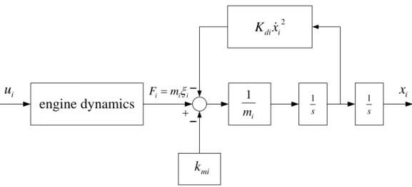
(16) 2.2 Vehicle Model. We assume that the road is horizontal, there is no wind gust, and all the vehicles travel in the same direction at all times. Fig. 2-2 shows the simplified vehicle 2. model of the ith vehicle in the platoon. The block ( K di x& i ) specifies the force due to the air resistance, where K di denotes the aerodynamic drag coefficient for the ith vehicle. ρAi C di / 2 , ρ. denotes the specific mass of air,. Ai. denotes the. cross-sectional area of the ith vehicle, and C di denotes the ith vehicle’s drag coefficient; Fi denotes the driving force produced by the ith vehicle’s engine; mi denotes the mass of the ith vehicle; ui denotes the throttle command input to the ith vehicle’s engine; and kmi denotes the ith vehicle’s mechanical drag. The longitudinal dynamics of the ith vehicle in the platoon are modeled as follows (for i=1,2,…,N) [1]: F u F&i = − i + i τ i ( x&i ) τ i ( x&i ). (2.2). mi &x&i = Fi − K di x&i − k mi. (2.3). 2. where τ i (.) denotes the engine time lag for the ith vehicle. Equation (2.2) described by a nonlinear differential equation represents the ith vehicle’s engine dynamics, and (2.3) represents Newtons’s second law applied to the ith vehicle modeled as a particle of mass mi. Differentiating both sides of (2.3) with respect to time, we have. mi&x&&i = F&i − 2 K di x&i &x&i. (2.4). 7.

(17) Substituting the expression for F&i by (2.2), (2.4) becomes mi&x&&i = −. Fi ui + − 2 K di x&i &x&i τ i ( x&i ) τ i ( x&i ). (2.5). from (2.3) and (2.5) we obtain &x&&i = −. K k  2 K di 1  1 &x&i + di x&i 2 + mi  − x&i &x&i + ui  τ i ( x&i )  mi mi  mi miτ i ( x&i ). (2.6). where &x&&i denotes the variation of the ith vehicle’s acceleration. Let xi = pi , x&i = vi , and &x&i = ai . The longitudinal ith vehicle dynamics can be written as p& i = vi   v&i = ai  a& = f (v , a ) + g (v )u i i i i i i  i. (2.7). where f i (vi , ai ) = − g i ( vi ) =. K di 2 k mi  2 K di 1  vi + vi a i −  ai + τ i ( vi )  mi mi  mi. and. 1 miτ i (vi ). The control objective is to keep ith vehicle follow it’s preceding vehicle and hold on a secure distance L, that is, xl − x1 = L, x1 − x2 = L, …, and x N −1 − x N = L . Namely, to input throttle command ui such that ∆ i can be driven to zero. At the same && are driven to zero, too. Meanwhile, we have changed a tracking time, ∆& i and ∆ i. problem to a regulator problem.. 8.

(18) K di x&i. ui. engine dynamics. Fi = miξi +. −. −. 1 mi. 2. 1 s. 1 s. xi. kmi Fig. 2-2 Simplified model of the ith vehicle in the platoon. 2.3 Power-Limited Acceleration. Maximum performance in longitudinal acceleration of a motor vehicle is determined by lots of limits; engine power is one of the most important factors of these limits. Fig. 2-3 [4] shows the performance characteristics of gasoline engine. Power and torque are related by the speed. Specifically, HorsePower(hp)=Torque(ft-lb) × Speed(rpm) ÷ 5252. (2.8). Power(kw)=0.746 × HorsePower(hp). (2.9). Also,. Thus, we obtain the reasonable range of ui is within 4000 N. Practically, with the advance of science and technology, maximum engine power limit is higher today.. 9.

(19) Fig. 2-3 Performance characteristics of gasoline engine [4]. 10.

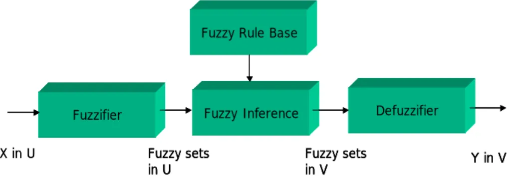
(20) Chapter 3 Fuzzy Logic Control. Fuzzy logic control is a useful methodology for system control in the presence of uncertainties and disturbances. The independence of expert knowledge of the controlled plants is a remarkable advantage in fuzzy logic controller (FLC) design. Besides, the control actions are usually smoothed through the well-built control rules. The basic principles of fuzzy logic were introduced by Zadeh in 1965, and the first application to the control of a dynamical process was reported by Mamdani in 1975. Because of the advantages such as easy implementation, suitability for complex dynamic systems, and high flexibility and robust nature, fuzzy controllers have been implemented in many fields [24-26]. The characteristic of FLC is that it adopts the linguistic control strategy to control plants without realizing their mathematical models. The linguistic control strategy of FLC is constructed according to the operator experience and/or expert knowledge. Experiences show that the FLC yields results superior to those obtained by traditional control algorithm in the complex situation where the system model or parameters are difficult to obtain. Typically, fuzzy controllers are based on four well-known stages: a fuzzification interface, a rule base, an inference engine, and a defuzzification interface as shown in Fig. 3-1. More detail descriptions for each stages are stated below.. 11.

(21) Fuzzy Rule Base. Fuzzifier X in U. Defuzzifier. Fuzzy Inference Fuzzy sets in U. Fuzzy sets in V. Y in V. Fig. 3-1 Fuzzy System Architecture 3.1 Fuzzy Set and Set-Theoretical Operators Definition 3.1 Fuzzy Set: Let U be a collection of objects, for example, U = R n , and be called the universe of discourse. A fuzzy set F in U is characterized by a membership function. µ F : U → [0,1] , with. µ F (u ) representing the grade of. membership of µ ∈U in the fuzzy set F. Definition 3.2 Support, Fuzzy Singleton: The support of a fuzzy set F is the point(s) u ∈ U at which µ F (u ) achieves its maximum value. If the support of a fuzzy set F is a. single point in U at which µ F = 1 , the F is called a fuzzy singleton. Definition 3.3 Intersection, Union, and complement: Let A and B be two fuzzy sets in U. The intersection A ∩ B of A and B is a fuzzy set in U with a membership function defined for all u ∈ U by µ A∩ B (u ) = min{µ A (u ), µ B (u )}. (3.1). The union of A ∪ B of A and B is a fuzzy set in U with the membership defined for all u ∈ U by 12.

(22) µ A∪ B (u ) = max{µ A (u ), µ B (u )}. (3.2). Usually, the intersection and union operators are denoted by ∧ and ∨ , respectively. The complement A of A is a fuzzy set in U with the membership function defined for all u ∈ U by. µ A (u ) = 1 − µ A (u ). (3.3). 3.2 Fuzzifiers The fuzzifier stage transforms crisp input from real values into fuzzy sets. Here we introduce three fuzzifiers as following: 1. Singleton fuzzifier: the singleton fuzzifier maps a real valued point x * ∈ U into the fuzzy singleton A in U, in which the membership value is 1 at x * and 0 at other points in U, i.e., 1 x = x * 0 otherwise. µ A ( x) = . (3.4). 2. Triangular fuzzifier: the triangular fuzzifier maps x * ∈ U into the fuzzy set A in U, in which the membership function is written as:  | x n − x n* | | x1 − x1* | ( 1 ) ( 1 ) if | x − x * |< bi , i = 1,2, K n − ⊗ ⊗ − L  µ A ( x) =  b1 bn 0 otherwise . (3.5). where bi are positive parameters and symbol ⊗ is often chosen as algebraic product or minimum. 3. Gaussian fuzzifier: the Gaussian fuzifier maps x * ∈ U into the fuzzy set A in U, in. 13.

(23) which the membership function is written as:. µ A ( x) = e. −(. x1 − x1*. δ1. )2. ⊗L⊗ e. −(. xn − xn*. δn. )2. (3.6). where δ i are positive parameters and symbol ⊗ is often chosen as algebraic product or minimum. Finally, we summarize the above fuzzifiers. The singleton fuzzifier greatly simplifies the computation involved in the fuzzy inference engine for all membership functions. And the Gaussian and triangular fuzzifiers do, too. The Gaussian and triangular fuzzifiers can restrain noise in the input, but the singleton fuzzifier cannot. 3.3 Deffuzzifiers The defuzzifier is defined as a mapping from a fuzzy set D in V ⊂ R to a crisp point y * ∈V . Hence, the task of the defuzzifier is to specify a point in V that represents the fuzzy set D. There are three types of defuzifiers introduced below. 1. Center of gravity Defuzzifier The center of gravity defuzzifier specifies y * as the center of the area covered by the membership function of D. y* =. ∫V yµ D ( y )dy , ∫V µ D ( y )dy. (3.7). where ∫V is the conventional integral. 2. Center Average Defuzzifier Let y l be the center of the lth fuzzy set and wl be its height. The center. 14.

(24) average defuzzifier presents y * as M. y* =. l ∑ y wl. l =1 M. (3.8). ∑ wl. l =1. 3. Maximum Defuzzifier The maximum defuzzifier chooses y * as the point in V, at which µ D ( y ) achieves its maximum value. Define hgt ( D ) = { y ∈ V | µ D ( y ) = sup µ D ( y )} . y∈V. (3.9). hgt(D) is a set of all point in V, at which µ D ( y ) achieves its maximum value. The maximum defuzzifier y * is defined as an arbitrary element in hgt(D), i.e., y * =any point in hgt(D).The mean of maximum defuzzifier is defined as:. y* =. ∫hgt yµ D ( y )dy ∫hgt µ D ( y )dy. (3.10). where ∫hgt ( D ) is an integration for the continuous part of hgt(D) and it is a summation for the discrete part of hgt(D). 3.4 Fuzzy Rule Bases The fuzzy rule base consists of fuzzy IF-THEN rules. It is the core of the fuzzy system in a sense. And all other stages are used to implement these rules in a reasonable and efficient manner. Hence, the fuzzy rule base comprises the following fuzzy IF-THEN rules: Rule i: IF x l is A1i and …and x n is Ani THEN y is D i. 15. (3.11).

(25) The canonical fuzzy IF-THEN rules in the form of (3.11) includes the following ones: (1) Partial rules: IF x1 is A1i and …and x m is Ami THEN y is D i. (3.12). (2) Or rules IF x1 is A1i and …and x m is Ami or x m +1 is Ami +1 and … x n is Ani THEN y is Di. (3.13). (3) Singles fuzzy statement y is D i. (3.14). 3.5 Fuzzy Inference The fuzzy inference is a reasoning method using the fuzzy theory, and whereby the expert knowledge is presented using linguistic rules. The fuzzy inference introduced as following. M. Product Inference: µ D ( y ) = max[sup( µ A ( x)∏ µ Al ( x i ) µ D ( y ))] l =1. x∈U. (3.15). i. M. Minimum Inference: µ D ( y ) = max[sup min( µ A ( x ), µ Al ( x1 )..., µ Al ( x n ), µ D l ( y ))] l =1. x∈U. 1. (3.16). n. The product inference and minimum inference are the most commonly used fuzzy inference in the fuzzy system and other fuzzy applications. In the Fig.3-2 shows the product inference and minimum inference [25-26].. 16.

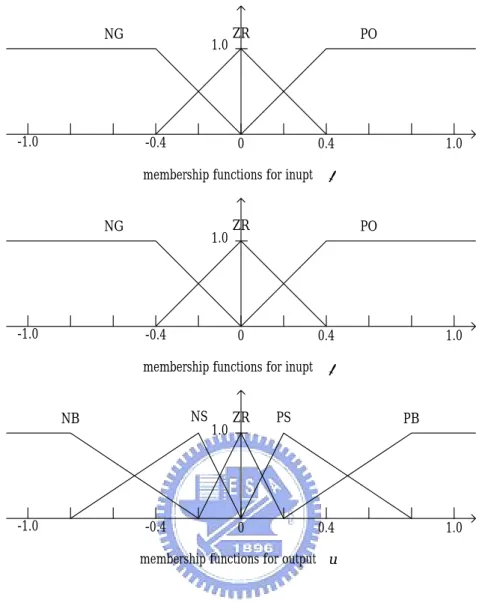
(26) y x. x. y x. x. Max. min Min. y (a) µ. µ. µ. y µ. x. x. µ. µ. y x. x. µ. Max. y (b) Fig. 3-2 (a) Minimum inference (b) Product inference. 3.6 Longitudinal Fuzzy Logic Control of a Platoon of Vehicles. In this section, we design a FLC by imitating a PD controller [6] for a platoon of vehicles. Design procedures are stated below. Step 1) Define ∆ i and ∆& i from Eq.(2.1) as two input variables of ith FLC; and ui as an output variable of ith FLC; the membership functions for input ∆ i , ∆& i and output ui are shown in Fig. 3-3.. 17.

(27) NG. -1.0. 1.0. -0.4. ZR. PO. 0. 0.4. membership functions for inupt. NG. -1.0. 1.0. -0.4. PO. 0. NS. -1.0. -0.4. 1.0. ∆. ZR. 0.4. membership functions for inupt. NB. ZR. 1.0. ∆&. PS. 0. 1.0. PB. 0.4. 1.0. membership functions for output u. Fig. 3-3 Membership function for input and output variables. Step 2) The main idea is : “ if ∆ i > 0 , input positive net force to decrease the space of two vehicles; if ∆ i < 0 , input negative net force to increase the space of two vehicles; ∆& i is used to amend the strategy above”. Table. 3-1 is the rule base we. obtain. Step 3) Select one type of the fuzzifiers, defuzzifiers, and fuzzy inferences. The most frequently used triangular membership, the center-of-gravity defuzzification, and the “max-min” reasoning method are adopted here to carry out the algorithm.. 18.

(28) ∆. ∆&. NG. ZR. PO. NG. NB. NS. ZR. ZR. NS. ZR. PS. PO. ZR. PS. PB. Table. 3-1 Rule Base of the Fuzzy Logic Controller. 3.7 Simulation Results. To examine the behavior of a platoon of vehicles under the above controller, we run simulations for a platoon consisting of 3 different types of vehicles. Three types of vehicles with their relevant parameters referring to [7][8] are shown in the Table. 3-2 and used in the simulations. In the simulation conducted, all the vehicles are assumed to be initially traveling at the steady-state velocity of v0 = 17.9 m/s (i.e., 40 mph). Beginning at time t = 0 s, the lead vehicle’s velocity is increased from its steady-state velocity value of 17.9 m/s until it reaches its final value of 21.9 m/s (i.e., 50 mph): the maximum jerk and the peak acceleration values corresponding to this velocity time profile are 0.5 m/s3 and 1m/s2 , respectively (see Fig. 3-4 and Fig. 3-5). Take three following vehicles as a simulation example, the order of vehicles in the. 19.

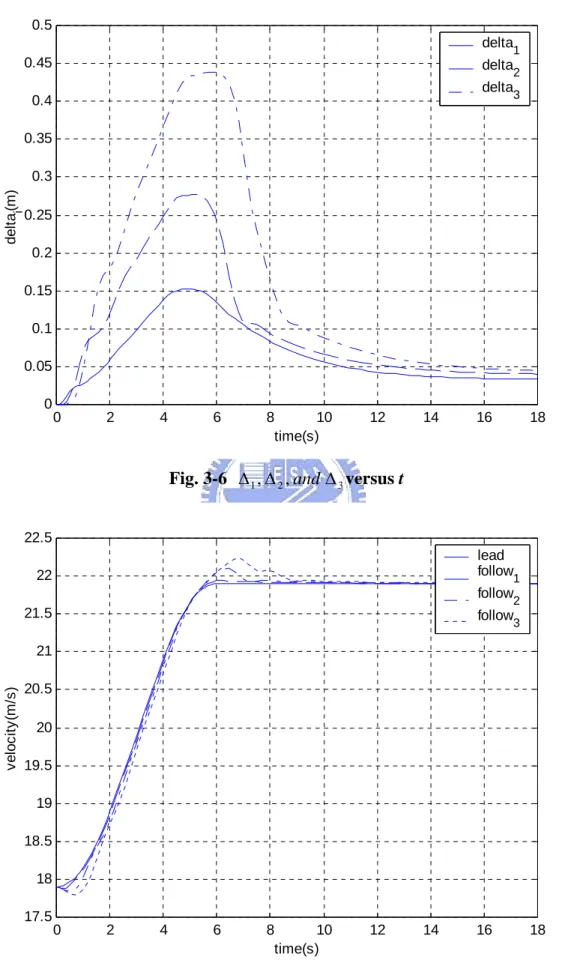
(29) platoon followed the lead vehicle is as follows: Daihatsu Charade CLS followed by Buick Regal Custom followed by BMW 750iL. Consider the vehicle loading, total mass of each following vehicle is conditioned by adding vehicle curb mass and passengers’ mass. Fig. 3-6 ~ Fig. 3-9 show the simulation results :. Type. Daihatsu Charade. Buick Regal. BMW 750iL. CLS. Custom. Vehicle i. 1. 2. 3. Curb mass(kg). 916. 1464. 1925. Passengers’ mass(kg). 91, 91, 91. 64, 64. 75. Vehicle mass mi(kg). 1189. 1592. 2000. Kdi(kg/m). 0.44. 0.49. 0.51. τ i (s). 0.2. 0.25. 0.2. kmi(N). 352. 392. 408. Table. 3-2 Simulation Model Parameters of Fuzzy Logic Control. 20.

(30) 22 21.5. lead vehicle velocity(m/s). 21 20.5 20 19.5 19 18.5 18 17.5 0. 2. 4. 6. 8 10 time(s). 12. 14. 16. 18. Fig. 3-4 Lead Vehicle’s velocity time profile: vl versus t 1 0.9. lead vehicle acceleration(m/s2). 0.8 0.7 0.6 0.5 0.4 0.3 0.2 0.1 0 0. 2. 4. 6. 8 10 time(s). 12. 14. 16. Fig. 3-5 Lead Vehicle’s acceleration time profile: al versus t 21. 18.

(31) 0.5 delta1 0.45. delta2 delta3. 0.4 0.35. deltai(m). 0.3 0.25 0.2 0.15 0.1 0.05 0 0. 2. 4. 6. 8 10 time(s). 12. 14. 16. 18. Fig. 3-6 ∆ 1 , ∆ 2 , and ∆ 3 versus t 22.5 lead follow1. 22. follow2 21.5. follow3. velocity(m/s). 21 20.5 20 19.5 19 18.5 18 17.5 0. 2. 4. 6. 8 10 time(s). 12. Fig. 3-7 vl , v1 , v 2 , and v3 versus t 22. 14. 16. 18.

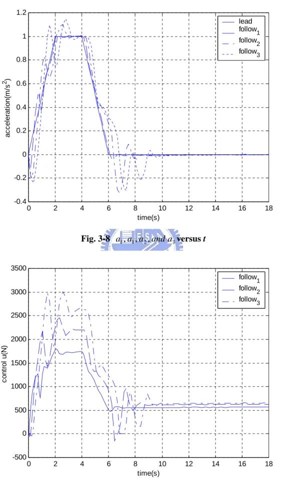
(32) 1.2 lead follow1. 1. follow2 follow3. acceleration(m/s 2). 0.8 0.6 0.4 0.2 0 -0.2 -0.4 0. 2. 4. 6. 8 10 time(s). 12. 14. 16. 18. Fig. 3-8 al , a1 , a 2 , and a3 versus t 3500 follow1 follow2. 3000. follow3 2500. control u(N). 2000 1500 1000 500 0 -500 0. 2. 4. 6. 8 10 time(s). 12. Fig. 3-9 u1 , u 2 , and u 3 versus t 23. 14. 16. 18.

(33) Chapter 4 H ∞ Observer-based Sliding Mode Control with Adaptive Fuzzy Neural Approach. 4.1 Fundamental Conceptions of Sliding Control Model imprecision, which is a common trouble in system control, can have strong adverse effects on nonlinear control systems. Therefore, any practical design must address it explicitly. A simple approach to robust control is the so-called sliding mode control (SMC) methodology. It allows an nth-order problem to be replaced by an equivalent 1st-order problem, which is intuitively easier to be addressed. For the class of systems to which it applies, sliding controller design provides a systematic approach to the problem of maintaining stability and consistent performance in the face of modeling imprecision. Take a single-input dynamic system for example: x ( n ) = f (x) + b(x)u. (4.1). where the scalar x is the output of interest, the scalar u is the control input, and x = [x. x& L x ( n −1) ]T is the state vector. In equation (4.1), f (x) (in general. nonlinear) is not exactly known, but the extent of the imprecision on f (x) is upper bounded by a known continuous function of x ; similarly, the control gain b(x) is not exactly known, but is of known sign and bounded by a known, continuous function of x . The control problem is to get the state x to track a specific 24.

(34) time-varying state x d = [ x d. x& d. L xd. ( n −1) T. ]. in the presence of model impression. on f (x) and b(x) . x = x − x d be the tracking error, and let Let ~ ~ x = x − x d = [~ x. ~ x& L ~ x ( n −1) ]T. (4.2). be the tracking error vector. Furthermore, let us define a time-varying surface s (t ) in the state-space R n by the scalar equation s (x; t ) = 0 , where  d s (x; t ) =  + λ    dt. n −1. ~ x,. (4.3). and λ is a strictly positive constant. The problem of tracking x ≡ x d is equivalent to that of remaining on the surface s (t ) for all t > 0 ; indeed s ≡ 0 represents a x ≡ 0 as t → ∞ . Thus, the linear differential equation whose unique solution is ~. problem of tracking the n-dimensional vector x d , i.e., the original nth-order tracking problem in x , can be replaced by a 1st-order problem of keeping the scalar quantity s at zero [11]. This simplified 1st-order problem of keeping s at zero can be. achieved by choosing the control law u such that outside of s (t ). 1 d 2 s ≤ −η s , 2 dt. (4.4). where η is a strictly positive constant [11]. Eq. (4.4) is called sliding condition. Essentially, (4.4) states that the squared “distance” to the surface, as measured by s 2 , decreases along all system trajectories.. 25.

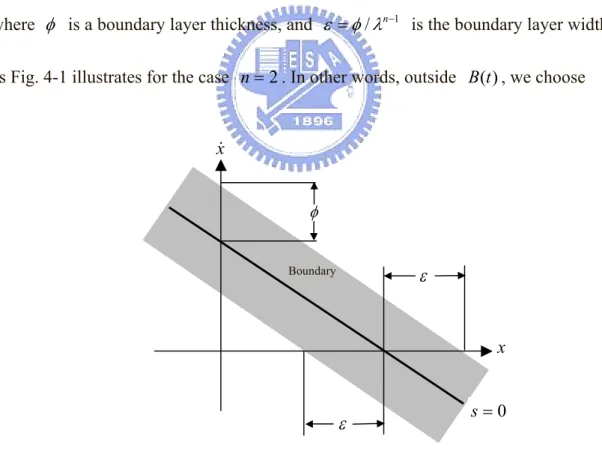
(35) However, in order to account for the presence of modeling imprecision and disturbances, the control has to be discontinuous across s (t ) . Since the implementation of the associated control switching is necessarily imperfect, this leads to chattering. In general, chattering must be eliminated for the controller to perform properly. This can be achieved by smoothing out the control discontinuity in a thin boundary layer neighboring the switching surface. B (t ) = {x, | s (x; t ) |≤ φ}. φ > 0,. (4.5). where φ is a boundary layer thickness, and ε = φ / λn −1 is the boundary layer width, as Fig. 4-1 illustrates for the case n = 2 . In other words, outside B (t ) , we choose. x& φ. ε. Boundary. x. ε. Fig. 4-1 Boundary layer. 26. s=0.

(36) u. φ. −φ. s. Fig. 4-2 Control interpolation in boundary layer. control u satisfying sliding condition (4.4), which guarantees that the boundary layer is attractive - hence invariant: all trajectories starting inside B(t=0) remain inside B(t) for all t ≥ 0 . Then, we interpolate u inside B(t), as illustrated in Fig. 4-2. This leads to tracking within a guaranteed precision ε (rather than “perfect” tracking), and in the meantime eliminates the chattering. 4.2 Sliding Mode Control. Let’s consider the first two vehicles in the forefront of the platoon. We will discuss the first couple of vehicles for detail thereinafter since the behavior of other couples of vehicles are similar. By rearranging (2.7) the first follow vehicle dynamic is written as. 27.

(37) p& 1 = v1   v&1 = a1  a& = f (v , a ) + g (v )u 1 1 1 1 1 1  1. (4.6). where f1 (v1 , a1 ) = −. g1 (v1 ) =. K d 1 2 k m1  2 K d 1 1  v1 + v1 a1 a1 + − m1 τ 1 (v1 )  m1  m1. and. 1 m1τ 1 (v1 ). And, the lead vehicle dynamic is stated as  p& l = vl   v&l = al a& = Va(t )  l. (4.7). where pl = xl , vl = x& l , al = &x&l , and Va is the variation of acceleration of the lead vehicle for increasing its velocity from v 0 to v f in a period of time. Substituting Eq. (4.6) and (4.7) to Eq. (2.1), we have &∆&& = Va(t ) − f (v , a ) − g (v )u 1 1 1 1 1 1. (4.8). && = e (3) , (4.8) is rewritten where ∆ 1 = xl − x1 − L . Let ∆ 1 = e1 (1) , ∆& 1 = e1 (2) , and ∆ 1 1. as e&1 (1) = e1 (2)   e&1 (2) = e1 (3)  e& (3) = Va(t ) − f (v , a ) − g (v )u 1 1 1 1 1 1 1. (4.9). where Va (t ) − f1 (v1 , a1 ) is a nonlinear function which depends on v1 and a1 , and u1. stands. for. the. control. input.. Let. F1 (v1 , a1 ) = Va (t ) − f1 (v1 , a1 ). G1 (v1 ) = − g1 (v1 ) . Therefore, (4.8) and (4.9) become 28. and.

(38) &∆&& = F (v , a ) + G (v )u 1 1 1 1 1 1 1. (4.10). e&1 (1) = e1 (2)   e&1 (2) = e1 (3)  e& (3) = F (v , a ) + G (v )u 1 1 1 1 1 1 1. (4.11). and. Let e 1= [e1 (1) e1 (2) e1 (3)] . The control target of this case is to find an appropriate T. control law u1 such that the tracking error e1 is zero. Furthermore, let the sliding surface s (t ) be expressed in the state-space R 3 by the scalar equation s(e 1 ; t ) = 0 as 2. d  s (e 1 ; t ) =  + λ  e1 (1) = e1 (3) + 2λ e1 ( 2) + λ2 e1 (1) , λ > 0  dt . (4.12). From (4.11), (4.12), and following similar derivations in [5], we can use the sliding mode control method and obtain a control law derived in Lemma 1. Lemma 1: Consider the nonlinear system (4.11) with given nonlinear function F1 (v1 , a1 ) . Suppose that control input is chosen as. u1 = G1 (v1 ) −1 [− F1 (v1 , a1 ) − λ2 e1 (2) − 2λe1 (3) − p 21e1 (1) − p 22 e1 (2) − k sign( s (e 1 ; t ))] (4.13) and that P is positive definite symmetric matrix, P ∈ R 2x2 satisfies the Lyapunov matrix equation T. A 1 P + PA 1 = −Q. (4.14). 29.

(39)  1 if s (e 1 ; t ) > 0 where sign( s (e 1 ; t )) =  − 1 if s (e 1 ; t ) < 0. ,.  0 A1 =  2 − λ. 1  is Hurwitz, p 21 , − 2λ . p 22 are elements of P, and Q > 0 is given. Then s → 0 and e 1 → 0 as t → ∞ .. □. Proof: From Eq.(4.12), we have e1 (3) = −λ2 e1 (1) − 2λe1 (2) + s . Let e1 = [e1 (1) e1 (2)]T , then  0 T e& 1 = [e1 (2) e1 (3)] =  2 − λ. 1  0  e1 +    − 2λ  s. (4.15). Consider a Lyapunov function candidate as following: v=. 1 2 1 T s + e1 P e1 2 2. (4.16). here P is positive definite symmetric matrix. By using (4.11), (4.12), (4.14), and (4.15), the time derivative of (4.16) is  0 T T v& = ss& + e1 P e& 1 = s[λ2 e1 (2) + 2λe1 (3) + F1 + G1u1 ] + e1 P(  2 − λ T T 0  = s[λ2 e1 (2) + 2λe1 (3) + F1 + G1u1 ] + e1 PA 1 e1 + e1 P   s = s[λ2 e1 (2) + 2λe1 (3) + F1 + G1u1 ] +. 1  0  e1 +   )  − 2λ  s. 1 T T T 0 e1 [PA 1 + A 1 P]e1 + e1 P   2 s. (4.17). Apply (4.13) to (4.17), we have the following relationship: 1 T 1 T v& = − ks ⋅ sign( s) − e1 Q e1 = −k s − e1 Q e1 < 0 ∀s ≠ 0 and e1 ≠ 0 2 2. (4.18). We conclude s → 0 and e1 → 0 (e 1 → 0) as t → ∞ . This completes the proof. □. Note that if we include the design of (4.5), (4.13) becomes 30.

(40) u1 = G1 (v1 ) −1 [− F1 (v1 , a1 ) − λ2 e1 (2) − 2λe1 (3) − p 21e1 (1) − p 22 e1 (2) − ksat ( s(e 1 ; t ) / φ )] ; φ > 0 (4.19)  s /φ if s / φ ≤ 1 where sat ( s (e 1 ; t ) / φ ) =  sign( s / φ ) otherwise. ,.  1 if ( s/φ ) > 0 sign( s/φ ) =  . − 1 if ( s / φ ) < 0 4.3 Sliding Mode Control with Fuzzy Neural Network Approximator. In practical applications, however, F1 (v1 , a1 ) is generally uncertain rather than given. The controller of (4.13) derived above is not always obtainable. Therefore, a new controller needs to be designed taking into account the unknown nonlinear function, which will be adequately approximated by a fuzzy-neural approximator. The configuration of the fuzzy-neural network shown in Fig. 4-3 consists of a fuzzy system and neural network. The fuzzy system can be divided into two parts: some fuzzy IF-THEN rules and a fuzzy inference engine. The fuzzy inference engine uses the fuzzy IF-THEN rules to perform a mapping from an input linguistic vector e 1 = [e1 (1) e1 (2) e1 (3)] ∈ R 3 to an output linguistic variable o(e 1 ) ∈ R . T. The ith fuzzy IF-THEN rule is written as Ri: If e1 (1) is A1i and e1 (2) is A2i and e1 (3) is A3i. than y i is B i. (4.20). where A1i , A 2i , A3i and B i are fuzzy sets with membership functions µ Ai (e1 ( j )) j. and µ B i ( y i ) . And y i is the point at which µ Bi ( y i ) = 1 . By using produce inference, center-average and singleton fuzzifier, the output of the fuzzy-neural network can be 31.

(41) expressed as. ϕ1. e1 (1). L A1i. y1. ϕ2. e1 ( 2). L A2i. y2. o (e 1 ). L. L ϕ. e1 (3). h. yh. L A3i. Layer I. Layer II. Layer III. Layer IV. Fig. 4-3 Configuration of a fuzzy-neural approximator.  3  i y ∏ µ Aij (e1 ( j )) ∑ i =1  j =1  o(e 1 ) = h  3  ∏ µ Aij (e1 ( j )) ∑ i =1  j =1  T = θ ϕ (e 1 ) h. (4.21). where µ Ai (e1 ( j )) is the membership function value of the fuzzy variable e1 ( j ) , j. h is the total number of the IF-THEN rules , y i is the point at which µ Bi ( y i ) = 1 , θ = [ y1. y 2 L y h ]T. is. an. adjustable. parameter. vector,. ϕ = [ϕ 1 ϕ 2 L ϕ h ]T is a fuzzy basis vector, where ϕ i is defined as 32. and.

(42) 3. ϕ (e 1 ) =. ∏µ j =1. i. Aij. (e1 ( j )).   3 ∏ µ Aij (e1 ( j )) ∑ i =1  j =1  h. .. (4.22). When the inputs are given into the fuzzy-neural network shown in Fig. 4-3, the truth value ϕ i (layer III) of the antecedent part of the ith implication is calculated by (4.22). Among the commonly used defuzzification strategies, the output (layer IV) of the fuzzy-neural network is expressed as (4.21). Therefore, the fuzzy logic approximator based on the neural network can be established. Fig. 4-3 shows the configuration of the fuzzy-neural function approximator. The approximator has four layers. At layer I, input nodes stand for the input linguistic variables e1 (1), e1 (2) , and e1 (3) . At layer II, nodes represent the values of the membership functions. At layer III, nodes are the values of the fuzzy basis vector ϕ . Each node of layer III performs a fuzzy rule. The links between layer III and layer IV are full connected by the weighting factors θ = [ y1. y 2 L y h ]T , i.e., the adjusted parameters. At layer IV, the output stands. for the value of o(e 1 ) . To approximate the uncertain nonlinear function F1 (v1 , a1 ) in (4.11), adaptive update laws to adjust the parameter vector θ in (4.21) of the fuzzy-neural approximator need to be developed. Let Fˆ1 be the estimation function for the uncertain nonlinear function F1 . That is, Fˆ1 (e 1 | θ) = θ T ϕ (e 1 ). (4.23) 33.

(43) In order to derive the adaptive update law, the following assumption is required. Assumption 1 [27]: Let e 1. belongs to a compact set U e1 = { e 1 ∈ R 3 : e 1 ≤ me1 < ∞. }. and me is. designed parameter. It is known a prior that the optimal parameter vector θ * = arg min[ sup F1 − Fˆ1 (e 1 | θ) ]. lies. θ∈M θ e ∈U 1 e1. M θ = { θ ∈ R 3 : θ ≤ mθ. } , where the radius. in. some. convex. region. mθ is constant.. □. Thus, to approximate the uncertain nonlinear term F1 , Eq. (4.10) becomes &∆&& = θ *T ϕ (e ) + G (v )u + w 1 1 1 1 1. (4.24). T. where w = F1 − θ * ϕ (e 1 ) is the lumped uncertainty. To facilitate the design process of the controller, the lumped uncertainty is generally assumed to have an upper bound, w ≤ wu ,. w u is a positive constant. (4.25). Based on above condition, a control law via fuzzy-neural approximator can be obtained from Lemma 2 below. Lemma 2: Consider the nonlinear system (4.11) with uncertain nonlinear function F1 (v1 , a1 ) , which is approximated as (4.24). Suppose Assumption 1 and (4.25) are. satisfied and control input is chosen as. 34.

(44) u1 = G1 (v1 ) −1 [−θˆ T ϕ (e 1 ) − λ2 e1 (2) − 2λe1 (3) − p 21e1 (1) − p 22 e1 (2) − k sign( s (e 1 ; t ))] (4.26) where θˆ is the estimate of θ * , and the update law is chosen as & θˆ = Γsϕ. (4.27). where Γ >0 is the adaptation matrix, k = k 2 + w u , k2>0, and s is the sliding surface. Then s → 0 and e 1 → 0 as t → ∞ . □. Proof: Consider the Lyapunov function v=. 1 2 1 T 1~ ~ s + e1 P e1 + θ T Γ −1 θ 2 2 2. (4.28). ~ where θ = θ * − θˆ .. The time derivative of (4.28) is v& = ss& +. 1 T & 1&T 1~ ~& 1 ~& ~ e1 P e1 + e1 P e1 + θ T Γ −1 θ + θ T Γ −1 θ 2 2 2 2. ~ & T = s[λ2 e&1 (1) + 2λe&1 (2) + e&1 (3)] + e1 P( A 1 e1 + [0 s ]T ) + θ T Γ −1 (−θˆ ) T 1 T ~ & T T = s[λ2 e1 (2) + 2λe1 (3) + θ* ϕ(e1 ) + G1 (v1 )u1 + w] + e1 (PA1 + A1 P)e1 + e1 P[0 s]T + θT Γ−1 (−θˆ ) 2. [. ]. = s λ2 e1 (2) + 2λe1 (3) + θ ∗T ϕ (e 1 ) + G1 (v1 )u1 + w − ~ & + s (e1 (1) p12 + e1 (2) p 22 ) − θ T Γ −1θˆ. 1 T & e1 Q e1 θˆ 2 (4.29). Apply (4.26) and (4.27) to (4.29), and let k = k 2 + w u , we have following relationship:. 35.

(45) 1 T ~ ~ & v& = s[ θ T ϕ (e 1 ) − p 21 e1 (1) − p 22 e1 (2) − k sign( s (e 1 ; t )) + w] − e1 Q e1 + s(e1 (1) p 21 + e1 (2) p 22 ) − θ T Γ −1θˆ 2 1 T ~ ~ = s[θ T ϕ (e 1 ) − k sign( s (e 1 ; t )) + w] − e1 Q e1 − θ T Γ −1 (Γsϕ (e 1 )) 2 = s [ − ( k 2 + w u ) sign ( s ) + w ] −. < −k 2 s −. 1 T e 1 Q e1 < 0 2. 1 T e 1 Q e1 2. ∀s ≠ 0 and e1 ≠ 0. (4.30). We conclude s → 0 and e 1 → 0 as t → ∞ . This completes the proof. □. 4.4 Sliding Mode Control with Fuzzy Neural Network Approximator and H ∞ performance As shown in (4.25) and (4.26), k = k 2 + w u needs to be determined in advance to construct the control input u1 , In practical applications, however, the exact upper bound w u cannot be chosen so as to attenuate the uncertainties, large control chattering nevertheless occurs. Simulation with a sliding mode controller illustrate this effects for different k selected. To relax the impractical constraint, a new control law is designed by using the H ∞ tracking design technique based on a much relaxed assumption [5], The lumped uncertainty is assumed such that w ∈ L2 [0, T ], ∀T ∈ [0, ∞). (4.31). Lemma 3: Consider the nonlinear system (4.11) with uncertain nonlinear function F1 (v1 , a1 ) , which is approximated as (4.24). Suppose Assumption 1 ,Eq. (4.25), and Eq. (4.31). 36.

(46) are satisfied; the control input is chosen as s u1 = G1 (v1 ) −1 [−θˆ T ϕ (e1 ) − λ2 e1 (2) − 2λe1 (3) − p 21e1 (1) − p 22 e1 (2) − ] 2ρ 2 (4.32) and the update law as (4.27), where ρ > 0 is the design constant serving as an attenuation level, s is the sliding surface. Then the H ∞ tracking performance [9], [10] for the overall system satisfies the following relationship: T 1 T T 1 1 T 1~ 1 ~ e1 Q e1 dτ ≤ s 2 (0) + e1 (0)P e1 (0) + θ T (0)Γ −1 θ (0) + ρ 2 ∫ w 2 (τ )dτ ∫ 0 2 0 2 2 2 2. (4.33) ~ where θ = θ * − θˆ .. □. Proof: Consider the Lyapunov function v=. 1 2 1 T 1~ ~ s + e1 P e1 + θ T Γ −1 θ 2 2 2. (4.34). The time derivative of (4.34) is (see (4.29)) T. v& = s[λ 2 e1 (2) + 2λe1 (3) + θ * ϕ (e 1 ) + G1 (v1 )u1 + w] −. 1 T ~ & e1 Q e1 + s (e1 (1) p12 + e1 (2) p 22 ) − θ T Γ −1θˆ 2. (4.35) Apply (4.27) and (4.32) to (4.35), we have v& =. −1 T 1 s 1 1 −1 T e1 Q e1 − ( − ρw) 2 + ρ 2 w 2 ≤ e1 Q e1 + ρ 2 w 2 2 2 ρ 2 2 2. By (4.31), we integrate (4.36) from t=0 to t=T, and obtain. 37. (4.36).

(47) T 1 T T 1 e1 (τ )Q e1 (τ )dτ ≤ v(0) + ρ 2 ∫ w 2 (τ )dτ ∫ 0 2 0 2. (4.37). Substituting (4.34) to (4.37), we have the H ∞ tracking performance, satisfying (4.33) T 1 T T 1 1 T 1~ 1 ~ e1 Q e1 dτ ≤ s 2 (0) + e1 (0)P e1 (0) + θ T (0)Γ −1 θ (0) + ρ 2 ∫ w 2 (τ )dτ ∫ 0 2 0 2 2 2 2. This completes the proof. □. Remark: If a set of initial condition e1 (0) = 0 , s (0) = 0 , θˆ (0) = θ * (0) can be obtained, and Q=I, then control performance of the overall system satisfies. sup w∈L2. where e1. 2 2. T. e1. w. = ∫ e1 (τ ) e1 (τ )dτ , w 0. T. 2 2. 2. ≤ρ. (4.38). 2 T. = ∫ w 2 (τ )dτ . That is, an arbitrary attenuation 0. level can be obtained, if ρ is adequately chosen. 4.5 Observer-based Sliding Mode Control with Fuzzy Neural Network Approximator and H ∞ performance. Utilizing sensors to obtain the measurements of the parameters in the vehicle system, such as the velocity, the acceleration,… etc., is difficult or expensive. Considering the technical difficulties and the economic benefits, we adopt an observer to estimate the plant output state vector while we assume that only the headway information of two vehicles is measurable. Under this constraint, a sliding mode 38.

(48) observer is proposed for state estimation [3][37]. The sliding observers offer advantages similar to those of sliding controllers such as robustness to parameter uncertainty and easy application to important classes of nonlinear systems. In this section, our task is to combine the plant and controller with an sliding observer which estimates the state vector e 1 ; the estimated vector is denoted as eˆ 1 and used as the input both of the sliding mode controller and of the adaptive fuzzy-neural network approximator instead of state feedback e 1 used before. Rewrite (4.11) as  e&1 (1) = e1 (2)   e&1 (2) = e1 (3) e& (3) = H (e , u ) 1 1 1 1. (4.39). where H 1 (e 1 , u1 ) = F1 + G1u1 . Consider the following observer [3][37][32]:  eˆ&1 (1) = eˆ1 (2) + λ1 sign(e1 (1) − eˆ1 (1))  &  eˆ1 (2) = eˆ1 (3) + λ 2 sign(e1 (1) − eˆ1 (1)) eˆ& (3) = H (eˆ , u ) + λ sign(e (1) − eˆ (1)) 1 1 1 3 1 1 1. (4.40). where eˆ 1 = [eˆ1 (1) eˆ1 (2) eˆ1 (3)]T are the observer output states; Po is positive definite symmetric matrix, Po ∈ R 2x2 satisfies the Lyapunov matrix equation T. A o P o + P o A o = −I  λ2 − λ o where A =  1  − λ3  λ1. (4.41).  1  is Hurwitz. Thus, the applied control to (4.39) and (4.40) is 0  39.

(49) solution of (4.32) replacing e 1 by eˆ 1 . Such an observer leads to the error ( ~e1 = e 1 − eˆ 1 ) dynamic of the form:  e~&1 (1) = e~1 (2) − λ1 sign(e~1 (1)) ~& ~ ~ e1 (2) = e1 (3) − λ 2 sign(e1 (1))  e~& (3) = ∆H − λ sign(e~ (1)) 1 3 1  1. (4.42).  1 if e~1 (1) > 0 where ∆H 1 = H 1 (e 1 , u1 ) − H 1 (eˆ 1 , u1 ) , and sign(e~1 (1)) =  ~ − 1 if e1 (1) < 0 .. Then, we assume that: Assumption 2: ∆H 1 (⋅) | ~e1 =0. is. globally. Lipschitz. continuous. in. its. first. argument. ∆H 1 (e 1 , u1 ) ≤ k 3 e 1 .. □. Assumption 3: 1 > P2o , where P2o is the 2nd column of matrix Po solution of (4.41). 2k 3 □. Theorem 1: Consider the nonlinear system (4.11) with uncertain nonlinear function F1 (v1 , a1 ) , which is approximated as (4.24). And with control defined as in Lamma 3,. to which observer (4.40) is associated. Suppose Assumption 1-3, (4.25), and (4.31) are satisfied. Then for any initial conditions, the state eˆ 1 of the observer converges toward the state e 1 of the system. □ 40.

(50) Proof: Consider. the. partial. Lyapunov. function. v=. 1~ 2 e1 (1) 2. leading. to. v& = e~1 (1)e~&1 (1) = e~1 (1)[e~1 (2) − λ1 sign(e~1 (1))] , with the constraint ~ e1 (2) max < λ1 we can obtain v& < ( ~ e1 (2) − λ1 ) ⋅ e~1 (1) < −σ e~1 (1) and ~ e (1) → 0. in finite time (t1). The. remaining estimation error can then be shown to decay exponentially using Filippov’s work. Taking a convex combination of the dynamics on each side, we have  e~&1 (1) = γ (e~1 (2) + λ1 ) + (1 − γ )(e~1 (2) − λ1 ) ~& ~ ~ e1 (2) = γ (e1 (3) + λ 2 ) + (1 − γ )(e1 (3) − λ 2 )  e~& (3) = γ (∆H + λ ) + (1 − γ )(∆H − λ ) 1 3 1 3  1. (4.43). For t＞t1, eliminating γ from above equations, (4.43) becomes   e~&1 (1) = 0  λ2 ~ ~& ~ ⋅ e1 (2) e1 (2) = e1 (3) − λ1  λ3 ~ ~& e1 (3) = ∆H 1 − λ ⋅ e1 (2) 1 . (4.44). Let e′1 = [e~1 (2) e~1 (3)]T . This is. e& 1′ = A o e1′ + [0 ∆H 1 (e1′ )]T. (4.45). Select Lyapunov function as V o = e1′ P o e1′ , T. T T T T V& o = 2e′1 P o e& ′1 = 2e′1 P o ( A o e′1 + [0 ∆H 1 (⋅)]T ) = 2e′1 P o A o e′1 + 2e′1 P o [0 ∆H 1 (⋅)]T. = −e′1 Ie′1 + 2e′1 P2o ∆H 1 (⋅) = − e′1 T. V& o ≤ − e′1. T. 2. + 2 e′1 P2o ∆H (⋅) ≤ − e′1. V& o ≤ −(1 − 2k 3 P2o ) e′1. 2. 2. 2. + 2e′1 P2o ∆H 1 (⋅) T. + 2 e′1 P2o k 3 e′1. ≤0. 41. (4.46).

(51) and thus ensures that e1′ decreases to zero □. Remark: In many applications, the sign(e~1 (1)) in (4.42) is replaced by a saturation function of the form. sign(e~1 (1)) if e~1 (1) > φ O ~ sat (e1 (1)) =  ~ O if e~1 (1) < φ O  e1 (1) / φ in order to remedy the control chattering [24]. Naturally, to prove asymptotic stabilization of the controlled plant plus the observer, we use the following Lyapunov function : W =. 1 2 1 T 1~ ~ sˆ + e′1′ Pe′1′ + θ T Γ −1 θ 2 2 2. (4.47). ~ where θ = θ * − θˆ , and e′1′ = [eˆ1 (1) eˆ1 (2)]T . Let sˆ = λ2 eˆ1 (1) + 2λeˆ1 (2) + eˆ1 (3) .. The time derivative of (4.47) is 1 T 1 T 1~ ~& 1 ~& ~ W& = sˆsˆ& + e′1′ Pe& ′1′ + e& ′1′ Pe′1′ + θ T Γ −1 θ + θ T Γ −1 θ 2 2 2 2 ~ & T = sˆ[λ2 eˆ&1 (1) + 2λeˆ&1 (2) + eˆ&1 (3)] + e′1′ P ( A 1 e′1′ + [0 sˆ]T ) + θ T Γ −1 (−θˆ ) T 1 T ~ & T T = sˆ[λ2 eˆ1 (2) + 2λeˆ1 (3) + θ* ϕ(eˆ 1 ) + G1uˆ1 + w] + e′1′ (PA1 + A1 P)e′1′ + e′1′ P[0 sˆ]T + θT Γ−1 (−θˆ ) 2 T 1 T ~ & = sˆ[λ 2 eˆ1 (2) + 2λeˆ1 (3) + θ * ϕ (eˆ 1 ) + G1uˆ1 + w] − e ′1′ Qe ′1′ + sˆ(eˆ1 (1) p12 + eˆ1 (2) p 22 ) − θ T Γ −1θˆ 2. (4.48) Apply. −1 uˆ1 = G1 [−θˆ T ϕ (eˆ 1 ) − λ2 eˆ1 (2) − 2λeˆ1 (3) − p 21eˆ1 (1) − p 22 eˆ1 (2) − k sign( sˆ(eˆ 1 ; t ))]. to (4.48), and let k = k 2 + w u , we have following relationship: 42.

(52) 1 T ~ ~ & W& = sˆ[ θ T ϕ (eˆ 1 ) − p 21 eˆ1 (1) − p 22 eˆ1 (2) − k sign( sˆ(eˆ 1 ; t )) + w] − e ′1′ Qe ′1′ + sˆ(eˆ1 (1) p 21 + eˆ1 (2) p 22 ) − θ T Γ −1θˆ 2 1 T ~ ~ = sˆ[θ T ϕ (eˆ 1 ) − k sign( sˆ(eˆ 1 ; t )) + w] − e ′1′ Qe ′1′ − θ T Γ −1 (Γsˆϕ (eˆ 1 )) 2 = sˆ[ − ( k 2 + w u ) sign ( sˆ ) + w ] −. 1 T e ′1′ Q e 1′′ 2. 1 T < − k 2 sˆ − e′1′ Qe′1′ < − k2 sˆ 2. < 0. (4.49). This completes the proof. □. 4.6 Simulation Results To examine the behavior of a platoon of vehicles under the above controller, we run simulations for a platoon consisting of 3 different types of vehicles again. Three types of vehicles with their relevant parameters are the same to the ones shown in the Table. 3-2 and are used in the simulations. In the simulation conducted, all the vehicles are assumed to be initially traveling at the steady-state velocity of v0 = 17.9 m/s (i.e., 40 mph). Beginning at time t = 0 s, the lead vehicle’s velocity is increased from its steady-state velocity value of 17.9 m/s until it reaches its final value of 21.9 m/s (i.e., 50 mph): the maximum jerk and the peak acceleration values corresponding to this velocity time profile are 0.5 m/s3 and 1m/s2 , respectively (also see Fig. 3-4 and Fig. 3-5). Take three following vehicles as an simulation example, the order of vehicles in the platoon followed the lead vehicle is as follows: Daihatsu Charade CLS followed by Buick Regal Custom followed by BMW 750iL. Consider the vehicle. 43.

(53) loading, total mass of each following vehicle is conditioned by adding vehicle curb mass and passengers’ mass. From Fig. 4-5 to Fig. 4-9 are the simulations of the application using a sliding mode controller with the boundary layer. From Fig. 4-10 to Fig. 4-14, we can see that the fuzzy neural approximator can approximate the uncertain nonlinear term of the system. From Fig. 4-15 to Fig. 4-19 , we apply the H ∞ performance with the control law obtained in section 4.3. It shows that the. performance is better and the chattering is attenuated, too. From Fig. 4-20 to Fig. 4-24, the observer is associated to estimate the system states, it shows that performance is still acceptable.. ∆( n ) = F + Gu + d. ∆ ~ ∆. + _. ∆ˆ. Observer. u. − Fˆ + (.....) u= G Controller. θ& = Γsϕ. Fˆ = θ T ϕ. Fig. 4-4 Block Diagram of Overall System. 44. ∆ˆ & ∆ˆ && ∆ˆ.

(54) symbols. parameters(values). λ. 1. λ1. 1. λ2. 2. λ3. 1. k. 1.2. ρ. 0.3. P21. 0.5. P22. 1.5. φ. 1.0. ∆ˆ 1 |t =0. -0.1. ∆ˆ 2 |t =0. 0.2. ∆ˆ 3 |t =0. 0.1. Γ1. 50I. Γ2. 40I. Γ3. 40I. Table. 4-1 Simulation Model Parameters of Modified Sliding Mode Control. 45.

(55) Fig. 4-5 ∆ 1 , ∆ 2 , and ∆ 3 versus t. Fig. 4-6 pl , p1 , p 2 , and p3 versus t. 46.

(56) Fig. 4-7 vl , v1 , v 2 , and v3 versus t. Fig. 4-8 al , a1 , a 2 , and a3 versus t. 47.

(57) Fig. 4-9 u1 , u 2 , and u 3 versus t. Fig. 4-10 ∆ 1 , ∆ 2 , and ∆ 3 versus t. 48.

(58) Fig. 4-11 pl , p1 , p 2 , and p3 versus t. Fig. 4-12 vl , v1 , v 2 , and v3 versus t. 49.

(59) Fig. 4-13 al , a1 , a 2 , and a3 versus t. Fig. 4-14 u1 , u 2 , and u 3 versus t. 50.

(60) Fig. 4-15 ∆ 1 , ∆ 2 , and ∆ 3 versus t. Fig. 4-16 pl , p1 , p 2 , and p3 versus t. 51.

(61) Fig. 4-17 vl , v1 , v 2 , and v3 versus t. Fig. 4-18 al , a1 , a 2 , and a3 versus t. 52.

(62) Fig. 4-19 u1 , u 2 , and u 3 versus t. Fig. 4-20 ∆ 1 , ∆ 2 , and ∆ 3 versus t. 53.

(63) Fig. 4-21 pl , p1 , p 2 , and p3 versus t. Fig. 4-22 vl , v1 , v 2 , and v3 versus t. 54.

(64) Fig. 4-23 al , a1 , a 2 , and a3 versus t. Fig. 4-24 u1 , u 2 , and u 3 versus t. 55.

(65) Chapter 5 Conclusions. In this thesis, we modeled mathematically both vehicle and car-following systems. In order to gain better performance and ensure the robustness and global stability, a sliding mode controller with the fuzzy-neural network approximator and H ∞ performance was proposed. Moreover, considering the technical difficulties and the economic benefits, we assumed that only the relative distance of two vehicles was measurable. Thus, an observer-based modified sliding mode controller was developed. The control performance of the proposed system were simulated. Simulation results demonstrated the validity and effectiveness of the controlled systems. The system with the modified sliding mode controller showed a better performance than the one controlled by a sliding mode controller did. With these two controllers, the robustness and the global stability were both guaranteed during the vehicles-following process in the presence of the uncertainties and disturbances. In designing the output feedback control law of an observer-based modified sliding mode controller, no differentiation of system outputs was performed in order to avoid the noise amplification associated with numerical differentiation, and no knowledge on nonlinearities of the nonlinear parts of the system was required. This. 56.

(66) controller is subject to on-line tuning for a nonlinear system. Although the performance of the car-following system with an observer is not as good as the one with a modified sliding mode controller which were combined with an aprroximator and H ∞ performance conception, it is still satisfying.. 57.

(67) References. [1]. Shahab Sheikholeslam and Charles A. Desoer, “Longitudinal control of a platoon of vehicles with no communication of lead vehicle information: a system level study,” IEEE Transactions on Vehicular Technology, Vol. 42, No. 4, pp.546-554, November 1993.. [2]. Michel Fliess, “Generalized controller canonical forms for linear and nonlinear dynamics,” IEEE Transactions on Automatic Control, Vol. 35, No. 9, pp.994-1001, September 1990.. [3]. W. Perruquetti, T. Floquet, and P. Borne, “A note on sliding observer and controller for generalized canonical forms,” Decision and Control, Proceedings of the 37th IEEE Conference on , Vol. 2 , pp.1920-1925, December 1998.. [4]. Thomas D. Gillespie, Fundamentals of Vehicle Dynamics, Warrendale, PA./Society of Automatic Engineers,Inc. 1992.. [5]. Wei-Yen Wang, Mei-Lang Chan, Chen-Chien James Hsu, and Tsu-Tian Lee, “ H ∞ tracking-based sliding mode control for uncertain nonlinear systems via an adaptive fuzzy-neural approach,” IEEE Transactions on Systems, Man, and Cybernetics – Part B: Cybernetics, Vol. 32, No. 4, pp.483 – 492, August 2002.. [6]. 孫宗瀛、楊英魁, Fuzzy 控制:理論、實作與應用, 全華科技圖書股份有限公司出版, 83 年 10 月 58.

(68) [7]. Shahab Sheikholeslam and Charles A. Desoer, “A system level study of the logitudinal control of a platoon of vehicles,” ASME J. Dynamic Systems, Measurement, and Control, Vol. 114, pp.286-292, June 1992.. [8]. Shahab Sheikholeslam and Charles A. Desoer, “Combined longitudinal and lateral control of a platoon of vehicles: a system level study,” PATH Technical Memorandum 91-3, September 1991.. [9]. Bor-Sen Chen, Ching-Hsiang Lee, and Yeong-Chan Chang, “ H ∞ tracking design of uncertain nonlinear SISO systems: Adaptive fuzzy approach,” IEEE Transactions on Fuzzy Systems, Vol. 6, No. 1, pp.32-43, February 1996.. [10] Wei-Yen Wang, Mei-Lang Chan, Tsu-Tian Lee, and Cheng-Hsin Liu, “Adaptive fuzzy control for strict-feedback canonical nonlinear systems with H ∞ tracking performance,” IEEE Transactions on Systems, Man, and Cybernetics – Part B: Cybernetics, Vol. 30, No. 6, pp.878 – 885, December 2000. [11] J. J. E. Slotine and Weiping Li, Applied nonlinear control, Englewood Cliffs, NJ: Prentice-Hall, 1991. [12] D. Yanakiev and I. Kanellakopoulos, “Longitudinal control of heavy-duty vehicles for automated highway systems,” Proceedings of the American Control Conference , Vol. 5, pp:3096-3100, June 1995 [13] L. X. Wang, Adaptive fuzzy systems and control: design and stability analysis,. 59.

(69) Englewood Cliffs, NJ: Prentice-Hall, 1994. [14] M. Tai and M. Tomizuka, “Robust longitudinal velocity tracking of vehicles using traction and brake control,” Advanced Motion Control, Proceedings of the 6th International Workshop on, pp:305 – 310, March/April 2000. [15] D. N. Godbole and J. Lygeros, “Longitudinal control of the lead car of a platoon,” IEEE Transactions on Vehicular Technology, Vol. 43, No. 4, pp.1125-1135, November 1994. [16] Chin-Teng Lin and C. S. George Lee, Neural fuzzy systems: a neuro-fuzzy synergism to intelligent systems, Upper Saddle River, NJ: Prentice Hall PTR, 1995 [17] 陳永平, 可變結構控制設計, 全華科技圖書股份有限公司出版, 88 年 9 月 [18] W. Wang, “Modeling scheme for vehicle longitudinal control,” Proceedings of the 31st IEEE Conference on Decision and Control, Vol. 1, pp:549-554, December 1992. [19] J. T. Spooner and K. M. Passino, “Stable adaptive control using fuzzy systems and neural networks,” IEEE Transactions on Fuzzy Systems, Vol. 4, pp.339-359, June 1996. [20] Li-Xin Wang, “Stable adaptive fuzzy controllers with application to inverted pendulum tracking,” IEEE Transactions on Systems, Man, and Cybernetics –. 60.

(70) Part B: Cybernetics, Vol. 26, No. 5, pp.677-691, October 1996. [21] Li-Xin Wang, “Stable adaptive fuzzy control of nonlinear systems,” IEEE Transactions on Fuzzy Systems, Vol. 1, No. 2, pp.146-155, May 1993. [22] Chih-Min Lin, C. F. Hsu, “Self-learning fuzzy sliding-mode control for antilock bracking systems,” IEEE Transactions on Control Systems Technology, Vol. 11, No. 2, pp.273-278, March 2003. [23] T. Hessberg, M. Tomizuka, “Fuzzy logic control for lateral vehicle guidance,” Second IEEE Conference on Control Applications, Vol. 2, pp.581-586, September 1993. [24] Y. G. Leu, T. T. Lee, and W. Y. Wang, “Observer-based adaptive fuzzy-neural control for unknown nonlinear dynamical systems,” IEEE Transactions on Systems, Man, and Cybernetics – Part B: Cybernetics, Vol. 29, No. 5, pp.583-591, October 1999. [25] C. C. Lee, “Fuzzy logic in control system: fuzzy logic controller-part I,” IEEE Transactions on Systems, Man, and Cybernetics, Vol. 20, pp.404-418, March/April 1990. [26] C. C. Lee, “Fuzzy logic in control system: fuzzy logic controller-part II,” IEEE Transactions on Systems, Man, and Cybernetics, Vol. 20, pp.419-435, March/April 1990.. 61.

(71) [27] K. S. Tsakalis and P. A. Ioannou, Linear Time-Varying Systems. Englewood Cliffs, NJ: Prentice-Hall, 1993. [28] Byung-Jae Choi, Seong-Woo Kwak, and Byung Kook Kim, “Design and stability analysis of single-input fuzzy logic controller,” IEEE Transactions on Systems, Man, and Cybernetics, Vol. 30, No. 2, pp.303-309, April 2000. [29] Ji-Chang Lo and Ya-Hui Kuo, “Decoupled fuzzy sliding-mode control,” IEEE Transactions on Fuzzy Systems, Vol. 6, No. 3, pp.426-435, August 1998. [30] Jacob S. Glower and Jeffrey Munighan, “Designing fuzzy controllers from a variable structures standpoint,” IEEE Transactions on Fuzzy Systems, Vol. 5, No. 1, pp.138-144, February 1997. [31] Byungkook Yoo and Woonchul Ham, “Adaptive fuzzy sliding mode control of nonlinear system,” IEEE Transactions on Fuzzy Systems, Vol. 6, No. 2, pp.315-321, May 1998. [32] Iqbal Husain, Sameer Sodhi, and Mehrdad Ehsani, “A sliding mode observer based controller for switched reluctance motor drives,” Industry Applications Society Annual Meeting , Conference Record of the 1994 IEEE , Vol. 1, pp.635-643, October 1994. [33] Cem Unsal and Pushkin Kachroo, “Sliding mode measurement feedback control for antilock braking systems,” IEEE Transactions on Control Systems. 62.

(72) Technology, Vol. 7, No. 2, pp.271-281, March 1999. [34] N. J. Schouten, M. A. Salman, and N. A. Kheir, “Fuzzy logic control for parallel hybrid vehicles,” IEEE Transactions on Control Systems Technology, Vol. 10, No. 3, pp.460-468, May 2002. [35] N. Jalil and N. Kheir, “Energy management studies for a new generation of vehicles (Milestone #5: Fuzzy logic for the series hybrid),” Tech. Rep., Dept. Elect. Syst. Eng., School Eng. Comput. Sci., Oakland Univ.,Rochester, MI, Mar. 1998. [36] N. Jalil and N. Kheir, “Energy management studies for a new generation of vehicles (Milestone #6: Fuzzy logic for the parallel hybrid),” Tech. Rep., Dept. Elect. Syst. Eng., School Eng. Comput. Sci., Oakland Univ.,Rochester, MI, Mar. 1998. [37] Ahmed-Ali and Francoise Lamnabhi-Lagarrigue, “Sliding Observer-Controller Design for Uncertain Triangular Nonlinear Systems,” IEEE Transactions on Automatic Contro, Vol. 44, No. 6, pp.1244-1249, June 1999.. 63.

(73)