Dynamic adjusting migration rates for multi-population genetic algorithms

(1)

Dynamically Adjusting Migration Rates for Multi-Population

Genetic Algorithms

Abstract

In this paper, the issue of adapting migration parameters for MGAs is investigated. We examine, in particular, the effect of adapting the migration rates on the performance and solution quality of MGAs. Thereby, we propose an adaptive scheme to evolve the appropriate migration rates for MGAs. If the individuals from a neighboring sub-population can greatly improve the solution quality of a current population, then the migration from the neighbor has a positive effect. In this case, the migration rate from the neighbor should be increased; otherwise, it should be decreased. According to the principle, an adaptive multi-population genetic algorithm which can adjust the migration rates is proposed. Experiments on the 0/1 knapsack problem are conducted to show the effectiveness of our approach. The results of our work have illustrated the effectiveness of self-adaptation for MGAs and paved the way for this unexplored area.

Keywords: Soft computing, genetic algorithm,

multi-population, parameter adaptation, migration rate.

1 Introduction

Genetic Algorithms (GAs) are robust search and optimization techniques that were developed based on the ideas and techniques from genetic and evolutionary theory. Historically, genetic algorithms are characterized as an evolutionary scheme performed on a single population of individuals.

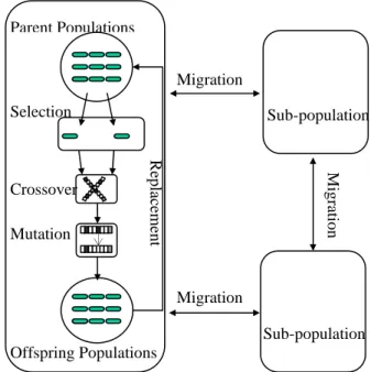
Multi-population genetic algorithms (MGAs) [7] is an extension of traditional single–population genetic algorithms (SGAs) by dividing a population into several sub-populations within which the evolution proceeds and individuals are allowed to migrate from one sub-population to another. This model is analogous to that used in parallel island GAs [2], without emphasizing the parallelism issue. Indeed, the MGA is more identical to the natural genetic evolution. For example, the human species consist of groups distant from each other while individuals within a group would migrate to another group. A typical MGA can be described as Figure 1. First, each sub-population evolves independently till some specific generations to reach the theoretical

equilibrium, resulting in many local optimal solutions in sub-populations. Each sub-population then migrates with its neighborhood(s). This punctuates the equilibrium and forces each sub-population evolving again to escape the local optimum and exploiting toward the global optimum.

Figure 1: A typical MGA with three sub-populations

Until recently, researchers have found that MGAs are more effective both in algorithmic cost and solution quality [6][10][13][14], such as:

1. It would shorten the number of generations needed to find the optimal or near optimal solution.

2. It usually can find more than one optimal solution.

3. It is more resistance to premature convergence. Despite of these advantages, the behavior and performance of MGAs are still heavily affected by a judicious choice of parameters, such as connection

topology (the topology that defined the connection

between the subpopulations), migration policy,

migration interval (a parameter that controls how

Tzung-Pei Hong, Wen-Yang Lin

Dept. of Computer Sci. and Info. Engineering

National University of Kaohsiung

Kaohsiung 811, Taiwan

tphong@nuk.edu.tw, wylin@nuk.edu.tw

Shu-Min Liu, Jian-Hong Lin

Dept. of Information Management

I-Shou University

Kaohsiung 840, Taiwan

Shumin.Liu@msa.hinet.net, jhlin@isu.edu.tw

Migration M ig ratio n Migration Sub-population Replacement Selection Mutation Parent Populations Offspring Populations Sub-population Crossover

(2)

often the migration occurs), migration rate (a parameter that controls how many individuals migrate), and population size (the number of subpopulations), etc. To our knowledge, most of the previous work focused on providing guidelines to choose those parameters empirically or rationally [3][4][13], and no work was devoted to the effect of adapting these parameters.

In this paper, the issue of adapting migration parameters for MGAs is investigated. We in particular examine the effect of adapting migration rates on performance and solution quality of MGAs. Thereby, we propose an adaptive scheme to evolve appropriate migration rates for MGAs. Experiments on the well-known 0/1 knapsack problem showed that our approach was superior to MGAs with static migration intervals and migration rates.

2 Previous Work

Grosso [8] was probably the first one that gives a systematic study of multi-population genetic algorithms. The MGA model he considered consisted of five subpopulations and each exchanged individuals with all the others with a fixed migration rate. With controlled experiments, he observed that the migration rate had great effect on the performance of MGAs. MGAs with migration rate below a critical point would have a similar effect to that with no migration at all.

Another study conducted by Pettey et al. [15] used a similar model but with different migration strategy. The migration occurs after each generational evolution, for which a copy of the best individual in each subpopulation is sent to all its neighbors.

In a parallel implementation of MGAs on a 4-D hypercube proposed by Tanese [17], migration occurred at fixed intervals between processors along one dimension of the hypercube. The migrants were chosen probabilistically from the best individuals in each subpopulation, and replaced the worst individuals in the receiving subpopulations. From experiments of different migration intervals, she observed that migrating too frequently or too infrequently degraded the performance of the algorithm. Another work of Tanese [18] showed that MGAs with migration performed significantly better than those without migration. Recently, a study conducted by Belding [1] using Royal Road function exhibited a similar conclusion.

In experiments with the parallel MGA, Cohoon et al. [6] noticed that there was relatively little change between migrations, but new solutions were found shortly after individuals were exchanged.

In the majority of multi-population GAs, migration is synchronous, which means that it occurs at predetermined constant intervals. Grosso [8] was also the first one to consider an asynchronous

migration scheme, where migration is enabled until the population was close to converge.

Braun [2] used the same idea and presented an algorithm where migration occurred after the populations converged completely. The same migration strategy was used later by Munetomo et al. [14], and so by Cant’u-Paz and Goldberg [5].

3 Experimental Analysis for Migration

Interval and Migration Rate

In this paper, we will study the effects of the two migration parameters, migration interval and

migration rate, on multi-population genetic

algorithms. Based on the effects, we will then propose promising adaptive algorithms to improve the performance of MGAs. In this section, we will discuss the influence of the two parameters through a wide variety of experiments on the 0/1 knapsack problem, which belongs to the class of knapsack-type problems and is well known to be NP-hard [11].

The 0/1 knapsack problem is stated as follows. Given a set of objects, ai, for 1 ≤ i ≤ n, together with

their profits Pi, weights Wi, and a capacity C, the 0/1

knapsack problem will try to find a binary vector x =

x1, x2, …, xn, such that: C W x n i i i⋅ ≤

∑

=1 , and

∑

= ⋅ n i i i P x 1 is maximal.

Following the suggestion made in [11], the data were generated with the following parameter settings:

v = 10, n = 250, Wi and Pi are random(1..v), and C =

2v, for which the optimal solution contained very few

items. Here, v is the maximum possible weight or

profit.

To facilitate the study, we consider the most adopted model of MGAs as shown in Figure 1 [2][9]. There are γ subpopulations, all of which are isolated and connected with as a ring structure. Individuals in MGA are migrated after every (migrate interval) generations and the best-worst migration policy is used [1][8][11]. That is, the best ρ (migration rate) of individuals in one subpopulation are selected to migrate to its neighbor subpopulations, and replace the worst individuals therein.

To be consistent with the crossover and mutation operators considered, the binary encoding scheme is used. Each bit represents the inclusion or exclusion of an object. It is, however, possible to generate infeasible solutions with this representation. That is, the total weights of the selected objects may exceed the knapsack capacity. In the literature, two different ways of handling this constraint violation [12] have been proposed. One way is to use a penalty function to penalize the fitness value of the infeasible candidate to diminish its chance of survival. Another approach is to use a repair mechanism to correct the representation of the infeasible candidate. In [12], the

(3)

repair method was more effective than the penalty approach. Hence, the repair approach is adopted in our implementation.

The repair scheme adopted here is a greedy approach. All the objects in a knapsack represented by an overfilled bit string are sorted in decreasing order of their profit-weight ratios. The last object is then selected for elimination (the corresponding bit of “1” was changed to “0”). This procedure is executed until the total weight of the remaining objects is less than the total capacity.

The parameters used in the proposed approach are set as follows.

♦ Number of populations: 16; ♦ Sub-population size: 30;

♦ Initial population: generated by random; ♦ Connection topology: ring;

♦ Crossover rate: 0.65; ♦ Mutation rate: 0.05;

♦ Selection method: tournament selection;

♦ Replacement method: keeping better individuals of old and new populations;

♦ Migration policy: selecting the best individuals to replace the worst ones of the neighbor sub-populations;

♦ Termination condition: 2000 generations; ♦ Number of experiments: 15 runs (get the average).

Different migration intervals and migration rates will be tested in the experiments.

The used multi-population genetic algorithm fixes both the migration intervals and migration rates. It is stated as follows.

The Multi-population Genetic Algorithm with Fixed Migration Intervals and Migration Rates:

Initialize the parameters;

Generate N sub-population P1, P2, …, PN randomly;

generation←1;

while generation≦max_gen do

for each sub-population Pi do

Use a fitness function to evaluate each individual in Pi;

Perform crossover in Pi; Perform mutation in Pi; Perform replacement in Pi; endfor generation←generation+1; if (generation % migration-interval ==0)

Perform migration at the fixed migration rate;

endwhile

To examine the performance of MGAs on different migration intervals and migration rates, the algorithm mentioned above is run with different combinations of constant migration intervals and migration rates. The test problem is the 0/1 knapsack problem. Experiments are first made to compare the solution quality along with different migration rates when the migration interval is fixed. The best fitness

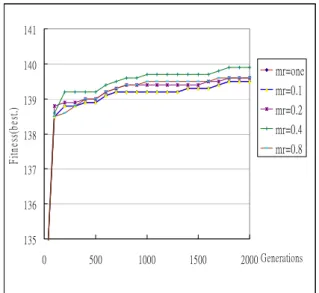
values for different migrate rates when the migration interval is fixed at 40 are shown in Figure 2. The line with mr = one individual represents one individual (the best one) is migrated each time the migration interval is reached and mr = 0.1 represents 10% of the

population will be migrated. In Figure 2, the line for

mr=one nearly completely overlaps with the line for mr=0.1. 135 136 137 138 139 140 141 0 500 1000 1500 2000 Generations Fi tn es s( be st .) mr=one mr=0.1 mr=0.2 mr=0.4 mr=0.8

Figure 2: The best fitness values for different migrate rates when the migration interval is fixed

at 40

It can be easily seen from Figure 2 that too high or too low migration rates will not cause the best fitness values. Instead, the middle migration rate 0.4 will get a good result in this case.

The average fitness values along with different migration rates are shown in Figure 3. Comparing Figures 2 and 3, it can be easily seen that the above conclusion is valid as well.

135 136 137 138 139 140 141 0 500 1000 1500 2000 Generations F itn es s( avg .) mr=one mr=0.1 mr=0.2 mr=0.4 mr=0.8

(4)

Figure 3: The average fitness values for different migrate rates when the migration interval is fixed

at 40

Next, experiments are made to compare the solution quality along with different migration intervals when the migration rate is fixed. The best fitness values for different migrate intervals when the migration rate is fixed at one individual being migrated are shown in Figure 4.

130 132 134 136 138 140 142 0 500 1000 1500 2000 Generations F itn ess( be st. ) mi= one mi= 10 mi= 20 mi= 40 mi= 80

Figure 4: The best fitness values for different migrate interval when the migration rate is fixed at

one individual

It can be easily seen from Figure 4 that different migration intervals may have their respective best fitness values in the genetic process.

The average fitness values along with different migration intervals are shown in Figure 5. Comparing Figures 4 and 5, it can be easily seen that the above conclusion is valid as well.

130 132 134 136 138 140 142 0 500 1000 1500 2000Generations F itn es s( av g. ) mi= one mi= 10 mi= 20 mi= 40 mi= 80

Figure 5: The average fitness values for different migrate intervals when the migration rate is fixed

at one individual

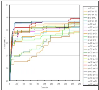
Next, different combinations of migration rates and migration intervals are compared. The experimental results for the best fitness values in the population are shown in Figure 6 Again, different combinations of migration intervals and migration rates may have the best effect in different stages of the genetic process. 135 136 137 138 139 140 141 0 200 400 600 800 1000 1200 1400 1600 1800 2000 Generation F itn ess( be st. ) mi=1/ mr=1 mi=1/ mr= 0.1 mi=1/ mr= 0.2 mi=1/ mr=0.4 mi=1/ mr= 0.8 mi=10/ mr=1 mi=10/ mr= 0.1 mi=10/ mr= 0.2 mi=10/ mr=0.4 mi=10/ mr= 0.8 mi=20/ mr=1 mi=20/ mr= 0.1 mi=20/ mr= 0.2 mi=20/ mr=0.4 mi=20/ mr= 0.8 mi=40/ mr=1 mi=40/ mr= 0.1 mi=40/ mr= 0.2 mi=40/ mr=0.4 mi=40/ mr= 0.8 mi=80/ mr=1 mi=80/ mr= 0.1 mi=80/ mr= 0.2 mi=80/ mr=0.4 mi=80/ mr= 0.8

Figure 6: The best fitness values for different combinations of migration intervals and migration

rates

The experimental results for the average fitness values in the population are shown in Figure 7.

135 136 137 138 139 140 141 0 500 1000 1500 2000 Generation fitn es s( av g. ) mi=1/ mr=1 mi=1/ mr= 0.1 mi=1/ mr= 0.2 mi=1/ mr=0.4 mi=1/ mr= 0.8 mi=10/ mr=1 mi=10/ mr= 0.1 mi=10/ mr= 0.2 mi=10/ mr=0.4 mi=10/ mr= 0.8 mi=20/ mr=1 mi=20/ mr= 0.1 mi=20/ mr= 0.2 mi=20/ mr=0.4 mi=20/ mr= 0.8 mi=40/ mr=1 mi=40/ mr= 0.1 mi=40/ mr= 0.2 mi=40/ mr=0.4 mi=40/ mr= 0.8 mi=80/ mr=1 mi=80/ mr= 0.1 mi=80/ mr= 0.2 mi=80/ mr=0.4 mi=80/ mr= 0.8

Figure 7: The average fitness values for different combinations of migration intervals and migration

rates

Traditional multi-population genetic algorithms use only a single migration interval and a migration

(5)

rate to exchange individuals among sub-populations and to prevent premature. The experimental results in this section show that different migration intervals and migration rates can, however, produce different fitness values, thus affecting the performance of the applied multi-population genetic algorithm. Designing a new multi-population genetic algorithm to automatically apply appropriate migration intervals and migration rates is then necessary.

4 The Proposed Migration-Rate Adjusting

Approach

If the individuals from a neighboring sub-population can greatly improve the solution quality of a current population, then the migration from the neighbor has a positive effect. In this case, the migration rate from the neighbor should be increased; otherwise, it should be decreased. According to the principle, an adaptive multi-population genetic algorithm which can adjust the migration rates is proposed as follows.

The Migration-Rate Adjusting Multi-population Genetic Algorithm:

Initialize the parameters;

Generate N sub-population P1, P2, …, PN randomly;

generation←1;

while generation≦max_gen do

for each sub-population Pi do

Use a fitness function to evaluate each individual in Pi; Perform crossover in Pi; Perform mutation in Pi; Perform replacement in Pi; endfor generation←generation+1; if (generation % migration-interval ==0)

Calculate the fitness increase new_FIi of

the best individual in each Pi ;

if (new_FIi > old_FIi)

increase the migration rate;

if (new_FIi < old_FIi)

decrease the migration rate;

Perform migration at the current migration rate;

endwhile

Note that in the above algorithm, the variable

old_FI represents the fitness increase in the last

migration interval. It is the difference of two fitness values in two neighboring migration intervals. Also different rules can be used to change the migration rate. The change may depend on the proportion of the fitness difference between two migration intervals or on a constant ratio.

5 Experimental Results

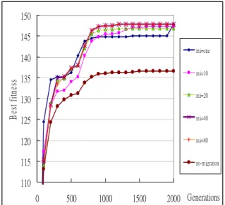
In this section, experiments are made for showing the performance of the proposed algorithm (4.1) for adjusting migration rates based on fitness values. The migration rates will be dynamically adjusted according to the improvement degrees from the neighbors. The initial migration rate is set at 0.4. Experimental results with dynamic migration and without migration are first compared. The fitness values are measured along different generations for migrations intervals fixed respectively at 1, 10, 20, 40 and 80. The experimental results for the best fitness values are shown in Figure 8.

110 115 120 125 130 135 140 145 150 0 500 1000 1500 2000 Generations B es t f itn es s mi=one mi=10 mi=20 mi=40 mi=80 no-migration

Figure 8: The best fitness values along with different generations for the above algorithm

It can be easily seen form Figure 8 that the experimental results with dynamic-rate migration are better than those without migration no matter what migration intervals are set at. The average fitness values along with different generations are shown in Figure 9. 80 90 100 110 120 130 140 150 0 500 1000 1500 2000Generations A vg fitne ss mi=one mi=10 mi=20 mi=40 mi=80 no-migration

(6)

Figure 9: The average fitness values along with different generations for the above algorithm

It can be seen that the results with dynamic-rate migration are also better than those without migration. Besides, when the migration interval is fixed at one (mi = one), the algorithm generates the best effect.

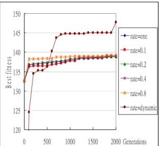
Next, experiments are made for comparing the performance with and without dynamic migration-rate adjusting. When the migration interval is fixed at one (mi = one), the results for different fixed migration rates (0.1、0.2、0.4、0.8、one individual) and for dynamic migration rates are shown in Figure 10.

120 125 130 135 140 145 150 0 500 1000 1500 2000 Generations B es t f itn es s rate=one rate=0.1 rate=0.2 rate=0.4 rate=0.8 rate=dynamic

Figure 10: The best fitness values for different fixed migration rates and for dynamic migration

rates when the migration interval is fixed at one

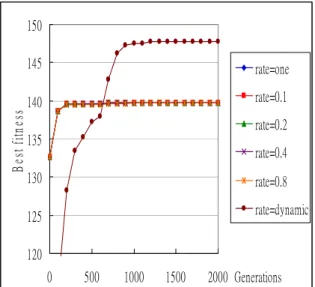
It can be easily seen from Figure 10 that the approach with dynamic migration-rate adjusting gets a better fitness value than those at fixed migration rates. The same experiments are then made for different intervals. When the intervals are set at 10, 20, 40 and 80, the results are respectively shown in Figures 11 to 13. 120 125 130 135 140 145 150 0 500 1000 1500 2000 Generations B es t fitn es s rate=one rate=0.1 rate=0.2 rate=0.4 rate=0.8 rate=dynamic

rates when the migration interval is fixed at 10

rates when the migration interval is at 20.

(7)

It can be concluded from these figures that the proposed algorithm has a good effect for all the different interval settings at 1, 10, 20, 40 and 80. The experimental results for the average fitness values are similar to the above ones.

6 Conclusions

In this paper, we have studied the issue of adapting migration parameters for MGAs, in particular, about how to adapt migration rates and migration intervals to improve performance and solution quality of MGAs. An adaptive scheme has been devised, which adjusts migration rates. A preliminary study on 0/1 knapsack problem has showed that the proposed adaptive approach can c o m p e t e w i t h a s t a t i c a p p r o a c h 120 125 130 135 140 145 150 0 500 1000 1500 2000 Generations B es t f itn es s rate=one rate=0.1 rate=0.2 rate=0.4 rate=0.8 rate=dynamic

with the best-tuned migration rate and migration interval.

As future works, we will conduct more experiments on other benchmarks, and devise methods to pursue an appropriate convergence threshold. We also will consider incorporating other representative parameters of MGAs, such as connection topology and migration policy, into our adaptive model.

Acknowledgements

This research was supported by the National Science Council of the Republic of China under contract NSC94-2213-E-390-005.

References

[1] T.C. Belding, “The distributed genetic algorithm revisited,” in Proceedings of the Sixth International Conference on Genetic Algorithms,

pp. 114-121, 1995.

[2] H.C. Braun, “On solving travelling salesman problems by genetic algorithms,” in

Proceedings of the First Workshop on Parallel Problem Solving from Nature, pp. 129-133, 1991.

[3] E. Cant'u-Paz, “A survey of parallel genetic algorithms,” Calculateurs Paralleles, Reseaux et Systems Repartis, Vol. 10, No. 2, pp. 141-171,

1998.

[4] E. Cant'u-Paz, “Migration policies and takeover time in parallel genetic algorithms,” in

Proceedings of Genetic and Evolutionary Computation Conference, 1999.

[5] E. Cant'u-Paz and D.E. Goldberg, “Efficient parallel genetic algorithms: Theory and practice,” Computer Methods in Applied Mechanics and Engineering.

[6] J.P. Cohoon, S.U. Hegde, W.N. Martin, and D.S. Richard, “Punctuated equilibria: A parallel genetic algorithm,” in Proceedings of the Second International Conference on Genetic Algorithms, pp. 148-154, 1987.

[7] J.P. Cohoon, W.N. Martin, and D.S. Richards, “Punctuated equilibria: A parallel genetic algorithm,” in Proceedings of the Second International Conference on Genetic Algorithms,

pp. 148-154, 1987.

[8] J.J. Grefenstette, “Parallel adaptive algorithms for function optimization,” Technical Report No. CS-81-19, Vanderbilt University, Computer Science Department, Nashville, TN, 1981. [9] P.B. Grosso, Computer Simulations of Genetic

Adaptation: Parallel Subcomponent Interaction in a Multilocus Model, Doctoral Dissertation,

The University of Michigan, 1985.

[10] S.C. Lin, W.F. Punch III, and E.D. Goodman, “Coarse-grain parallel genetic algorithms: categorization and new approach,” in

Proceedings of the Fifth International Conference on Genetic Algorithms, pp. 28-37,

1994.

[11] S. Martello and P. Toth, Knapsack Problems,

Jonh Wiley, UK, 1990.

[12] Z. Michalewicz, Genetic Algorithms + Data Structures = Evolution Programs,

Springer-Verlag, 1994.

[13] H. Muhlenbein, M. Schomisch, and J. Born, “The parallel genetic algorithm as function optimizer,” in Proceedings of the Fourth

International Conference on Genetic Algorithms,

(8)

[14] M. Munetomo, Y. Takai, and Y. Sato, “An efficient migration scheme for subpopulation-based asynchronously parallel genetic algorithms,” in Proceedings of the Fifth International Conference on Genetic Algorithms,

1993.

[15] C.B. Pettey, M.R. Leuze, and J.J. Grefenstette, “A parallel genetic algorithm,” in Proceedings of the Second International Conference on Genetic Algorithms, pp. 155-161, 1987.

[16] D. Schlierkamp-Voosen and H. Muhlenbein, “Adaptation of population sizes by competing subpopulations,” in Proceedings of IEEE International Conference on Evolutionary Computation, pp. 330-335, 1996.

[17] R. Tanese, “Parallel genetic algorithm for a hypercube,” in Proceedings of the Second International Conference on Genetic Algorithms,

pp. 434-439, 1987.

[18] R. Tanese, “Distributed genetic algorithms,” in

Proceedings of the Third International Conference on Genetic Algorithms, pp. 177-183,