創新動態中的最佳化能力集合轉化

全文

(1)國立交通大學資訊管理研究所博士論文. 創新動態中的最佳化能力集合轉化 Optimal Transformation of Competence Set in Innovation Dynamics. 研究生：賴宗智指導教授：游伯龍. 教授. 中華民國九十七年六月.

(2) 創新動態中的最佳化能力集合轉化 Optimal Transformation of Competence Set in Innovation Dynamics. 研究生：賴宗智. Student：Tsung-Chih Lai. 指導教授：游伯龍. Advisor：Po-Lung Yu. 國立交通大學資訊管理研究所博士論文. A Dissertation Submitted to Institute of Information Management College of Management National Chiao Tung University in Partial Fulfillment of the Requirements for the Degree of Doctor of Philosophy in. Information Management June 2008 Hsinchu, Taiwan, Republic of China. 中華民國九十七年六月.

(3) 創新動態中的最佳化能力集合轉化研究生：賴宗智. 指導教授：游伯龍. 教授. 國立交通大學資訊管理研究所. 中文摘要. 我們的記憶、觀念、想法、判斷、反應（統稱為念頭和思路）雖然是動態的，但經過一段時間以後，如果沒有重大事件的刺激，會漸漸地穩定下來，而停在一個固定的範圍內。這些念頭和思路的綜合範圍，包括它們的動態和組織，就是我們的習慣領域（habitual domain, HD）。當我們面對一個決策問題時，相對應的存在一個能力集合（competence set, CS），包括能使我們得到滿意解答所須的想法、知識、技能、資源等等。因為能力集合是我們習慣領域針對某一決策問題的投影，如果習慣領域僵化了，我們的能力集合便無法擴展，進而會阻礙創新的展現。若沒有持續不斷地擴展、升級我們的習慣領域與能力集合，我們就很有可能走入決策陷阱或做出錯誤的決策而不自知。本論文基於習慣領域理論及能力集合分析，提出運作領域（working domain）的概念以及創新循環模式（innovation dynamics）。此模式可以使我們的運作領域能更加的靈活、有彈性。接著我們將著眼於創新循環模式中能力集合轉化的部份，討論最佳化能力集合調整問題。給定一個目標解，我們提出能力集合調整模式（competence set adjustment model, CSA model）求得生產參數的最佳調整，使得該目標解得以被達成。當目標解無法被達成時，我們透過二分法（bisection algorithm）或模糊線性規劃（fuzzy linear programming）的方法修正此目標解。最後，我們利用多準則多資源水準限制線性規劃模式（multiple criteria and multiple constraint levels linear programming, MC2LP）探討可變生產參數的線性規劃模式。這些參數包括單位利潤、可用資源以及投入產出參數。在這些參數會隨著投資或時間而改變的情況下，我們將探討如何找到動態最佳解使得「接單時虧損，交貨時獲利」（紅色接單、黑色出貨）的目標得以實現。. 關鍵詞：習慣領域、能力集合、創新動態、能力集合調整、多目標決策、多準則多資源水準限制數學規劃、紅色接單黑色出貨. -i-.

(4) Optimal Transformation of Competence Set in Innovation Dynamics Student：Tsung-Chih Lai. Advisor：Dr. Po-Lung Yu Institute of Information Management National Chiao Tung University. Abstract Habitual domain (HD) is a collection of ways of thinking, coupled with its formation, interaction and dynamics, which can gradually stabilize as time passes. Unless extraordinary events occur, our thinking process will reach a steady state. For a decision problem E, there exists a corresponding competence set (CS) consisting of ideas, knowledge, skills, and resources to successfully solve the problem. Being a projection of our habitual domains with respect to E, our competence set may not be expanded as our habitual domains get ossified. This can conceal our innovation. Therefore, without continuous expanding and upgrading our HD and CS, we may unconsciously step into decision traps and make wrong decisions. Based on HD theory and CS analysis, the dissertation presented here introduces the concepts of working domain and innovation dynamics. The model of innovation dynamics helps our working domain become more flexible and agile. We, in advance, focus on the transformation of competence set in the innovation dynamics to investigate the problem of optimal adjustment of competence set. The program is formulated into a linear programming model called competence set adjustment model (CSA model). By means of the CSA model, we study how to optimally adjust the relevant coefficients so that a given target solution could be attainable. In case the target is unattainable, we may either utilize the bisection method or the fuzzy linear programming techniques to revise the target as to make it a reachable one. Finally, we utilize multiple criteria and multiple constraint levels linear programming (MC2LP) model and its extended techniques to explore the linear programming models with changeable parameters. The parameters include: unit profit, available resources and input-output coefficients of production function. With those parameters changed with capital investment and/or time, we study how to find dynamic best solutions to make "taking loss at the ordering time and making profit at the time of delivery" feasible. For more general cases we also sketch a generalized mathematical programming model with changeable parameters and control variables. Keywords: Habitual Domains, Competence Set Analysis, Innovation Dynamics, Competence Set Adjustment, Multiple Criteria Decision Making, Multiple Criteria and Multiple Constraint Levels Linear Programming, Red in-Black out -ii-.

(5) 誌. 謝. 本論文得以順利完成，首先得感謝游伯龍教授的悉心指導。在國立交通大學碩、博士班修業的八年當中，幸有游老師不時花費時在觀念上進行討論，才得以有今天的成果。在平時的討論中，游老師就有如良師益友般，時常給予我精神上的鼓勵與肯定，並常提供、分享一些以往的求學經驗，解除了我在求學路上的迷惑。游老師宏觀的視野與嚴謹的研究態度，著實使我獲益良多。在此謹致上我最深及最誠摯的感謝之意。. 同時由衷地感謝口試委員王小璠老師、曾國雄老師、姜林杰祐老師、黎漢林老師、林妙聰老師與李永銘老師對於本論文提供寶貴的指教與建議，使得本論文不完美之處得以更加完整，在此亦致上對口試委員們的謝意。. 除了師長們在研究上的教導與指正，在此同時感謝同研究室的學弟妹們，彥曲、靜芳及鴻順在日常生活上的相互扶持。本所諸位優秀的同窗夥伴們，俊龍、嘉輝、韓英、勇紹、美靜、韻嵐等人，有你們的陪伴使我在漫長的研究路上不感孤單。在研究期間於學業與生活上的低潮時刻，感謝鼎元、友義在我心煩與精神不濟時對我的關懷與信心喊話。也謝謝本所助理淑惠在許多事務上給予協助。. 最後，更要感謝我的父母與家人在我研究期間的支援，以及妻子翠玲的鼓勵與支持，讓我能夠無後顧之憂地攻讀學位。如今，完成學業、論文付梓，謹獻上最真誠的謝意給我親愛的家人，並他們分享這喜悅的一刻。本論文謹獻給任何幫助我的朋友們。謝謝您們。. 賴宗智國立交通大學資訊管理研究所中華民國九十七年六月. -iii-.

(6) TABLE OF CONTENTS. 中文摘要 .....................................................................................................................................i Abstract .....................................................................................................................................ii 誌. 謝 .......................................................................................................................................iii. TABLE OF CONTENTS ........................................................................................................iv LIST OF FIGURES ................................................................................................................vii LIST OF TABLES ...................................................................................................................ix CHAPTER 1 INTRODUCTION.............................................................................................1 1.1 Research Background ...................................................................................................1 1.2 Motivation and Objective .............................................................................................3 1.3 Overview of Dissertation..............................................................................................5 CHAPTER 2 LITERATURE REVIEW ON HABITUAL DOMAINS THEORY AND COMPETENCE SET ANALYSIS ..........................................................................................8 2.1 Habitual Domains Theory ............................................................................................8 2.1.1 Behavior Mechanism.........................................................................................9 2.1.2 The Four Basic Elements of Habitual Domain................................................13 2.1.3 Degree of Habitual Domain Expansion...........................................................15 2.2 Competence Set Analysis ...........................................................................................17 2.2.1 α-core Competence Set....................................................................................18 2.2.2 Four Elements of Competence Set ..................................................................19 2.2.3 Classification of Decision Problems ...............................................................21 CHAPTER 3 WORKING DOMAIN AND INNOVATION DYNAMICS .........................24 3.1 Property of the Activation Probability........................................................................24 3.2 Working Domain ........................................................................................................27. -iv-.

(7) 3.3 Classification of Decision Problems...........................................................................29 3.4 How Working Domain Get Trapped...........................................................................31 3.5 Innovation Dynamics..................................................................................................34 CHAPTER 4 OPTIMAL ADJUSTMENT OF COMPETENCE SET WITH LINEAR PROGRAMMING..................................................................................................................40 4.1 Introduction to Optimal Competence Set Adjustment Problems ...............................40 4.2 Problem Statement......................................................................................................42 4.3 Optimal Adjustment of Competence Set ....................................................................45 4.4 Bisection Algorithm....................................................................................................51 4.5 Target Revision by the Fuzzy Linear Programming...................................................56 CHAPTER 5 LINEAR PROGRAMMING MODELS WITH CHANGEABLE PARAMETERS - THEORETICAL ANALYSIS ON "TAKING LOSS AT THE ORDERING TIME AND MAKING PROFIT AT THE DELIVERY TIME" ..................61 5.1 Introduction to Linear Programming Models with Changeable Parameters ..............62 5.2 Preliminary: MC2-simplex Method ............................................................................63 5.3 Parameter Changes through Investment on Resources and Marketing ......................66 5.3.1 A Concrete Example ........................................................................................67 5.3.2. Parameter Changes by Investment in Resources and Markets .......................74 5.4 “Red in-Black out” Phenomenon-Parameter Changes in c and d due to Time Advancement ............................................................................................................................76 5.4.1. An Illustrative Example ..................................................................................76 5.4.2. Generalized Model for Parameter Changes in c and d due to Time Advancement ....................................................................................................................80 5.5 Generalized Model for Parameter Changes Including Elements of A........................86 5.5.1. An Illustrative Example ..................................................................................86 5.5.2. A Generalization, Including Changes in Elements of A .................................88 5.5.3. Further Generalization with Parameters as Control Variables........................91. -v-.

(8) CHAPTER 6 CONCLUSIONS AND REMARKS ..............................................................93 ACKNOWLEDGEMENTS ...................................................................................................96 REFERENCES .......................................................................................................................96 Appendix 1 Behavior Mechanism – 8 hypotheses..............................................................104 Appendix 2 Eight Methods for Expansion of Habitual Domains.....................................106 Appendix 3 Nine Principles of Deep Knowledge ...............................................................108 Appendix 4 Seven Self-perpetuation Operators ................................................................ 110. -vi-.

(9) LIST OF FIGURES. Figure 1-1 Two domains of competence set analysis [10]. ........................................................3 Figure 1-2 The organization of the dissertation..........................................................................7 Figure 2-1 The behavior mechanism [11]................................................................................. 11 Figure 2-2 A vivid illustration of PDt, RDt, and ADt. ...............................................................15 Figure 2-3 Illustration of α-core competence set [12]. .............................................................19 Figure 2-4 Four basic elements of competence set and their relationships [12]. .....................20 Figure 2-5 Routine problems....................................................................................................21 Figure 2-6 Trt(E) is only fuzzily known. ..................................................................................22 Figure 2-7 Competence set of challenging problems. ..............................................................23 Figure 3-1 The activation probability for circuit patterns at t1. ................................................25 Figure 3-2 The activation probability for circuit patterns at t2. ................................................25 Figure 3-3 The activation probability for circuit patterns at t3. ................................................26 Figure 3-4 The activation probability for circuit patterns at t3 when the activation continuity assumption is held. ...........................................................................................................27 Figure 3-5 Multiple-component model of working memory [24]............................................28 Figure 3-6 Clockwise Innovation Dynamics. ...........................................................................36 Figure 3-7 Counter-clockwise Innovation Dynamics...............................................................38 Figure 4-1 Graphical representation of the optimal adjustment of competence set in Example 4.1. ....................................................................................................................................51 Figure 4-2 Graphical representation of the bisection method. .................................................53 Figure 4-3 Flow chart of the Algorithm 4.1. ............................................................................54 Figure 4-4 The membership functions of the fuzzy sets Ã and b ...........................................58 Figure 5-1 The potential solution structure of model (35) when y and z are not limited. ........72 Figure 5-2 The potential solution structure of model (35) with investment constraints (36)...73 -vii-.

(10) Figure 5-3 Trends of optimal solutions and objective values at different time interval...........78 Figure 5-4 Intersecting points of the line of y=z with the potential solution structure in parameter space. ...............................................................................................................80 Figure 5-5 Two situations for sj to be an empty set. .................................................................83 Figure 5-6. Flow chart of Algorithm 5.4.1. ..............................................................................85. -viii-.

(11) LIST OF TABLES. Table 2-1 A structure of goal functions [12].............................................................................12 Table 2-2 Eight basic methods for expanding habitual domains..............................................17 Table 2-3 Nine principles for deep knowledge.........................................................................17 Table 4-1 Optimal adjustment of competence set with different α values...............................60 Table 5-1 Unit profits, resource consumption rates and available resource levels in Example 5.3.1 ..................................................................................................................................67 Table 5-2 Profit rates and resource levels change for each unit of investment. .......................68 Table 5-3 MC2-simplex tableaus for the potential bases of model (35). ..................................70 Table 5-4 The optimal parameter spaces for the potential solutions of model (35). ................71 Table 5-5 Example 5.4.1 in a nutshell. .....................................................................................77 Table 5-6 The optimal solutions and their objective values for different t values for (41). .....77 Table 5-7 A summary of the problem of Example 5.5.1...........................................................86. -ix-.

(12) CHAPTER 1 INTRODUCTION. 1.1 Research Background In the last few decades, habitual domains (HDs) theory has attracted enormous managers and researchers to study it. HDs theory can be of help in developing leadership skills [1], generating innovative ideas [2], preventing from decision traps [3], and forming winning strategies [4]. Having also noticed the benefit of the HDs theory to fundamental education, the Ministry of Education in Taiwan funded the seed teacher training program of HDs in 2007 and 2008. More than 120 teachers, mostly from center of general education, have plunged into researching and/or teaching the HDs theory. Undoubtedly, the importance of HDs theory has increased day by day.. The concept of HDs was initiated by Yu [5]. Its main idea is that the set of ideas and knowledge which are stored in our mind can gradually stabilize over a period of time. Unless extraordinary events occur, our thinking process will reach some steady state [6]. This phenomenon continuously takes place in our daily life. For example, someone learns how to drive a car. At the beginning, he/she may feel that controlling a car is quite difficult. However, after times of practice, he/she may feel more comfortable to drive a car (a steady state).. Our habitual domains can be stabilized. This can be mathematically proved [7] based on commonly observed facts:. 1.. The more we learn, the less the likelihood that an arriving event or piece of information is new to us.. -1-.

(13) 2.. To interpret arriving events, we tend to relate them to past experiences.. 3.. We tend to look for rhythms in our lives and force arriving events to conform to those rhythms.. Our HDs go wherever we go and have great impact on our decision making both individual level and organizational level.. From the individual point of view, given a decision problem or event E we need a set of ideas, knowledge, skills, and resources that could be of help to obtain a satisfactory solution. The set is called a competence set (CS), denoted by CS(E). The concept of CS is also proposed by Yu [8], [9]. As an extension of HDs, a competence set is a projection of our habitual domains with respect to E. Once we have acquired the competence set, CS(E), it could be transformed into services or products to relieve pains and frustrations.. Each organization, in abstract, is a living entity and hence has its HD and CS. If the organization wants to be more competitive than its competitors, its CS must be adequately flexible and adaptable. That is, to be powerful, the organization should abidingly create new product or service which fulfills target customers’ requirements by the fusion of innovative ideas and the required resources. The process must be flexible and adaptable so that the CS of the organization can be properly adjusted according to both internal and external environment changes.. Competence set analysis (CSA) contains two inherent domains: competence domain and problem domain. As shown in Figure 1-1, there are two kinds of short-term problems in CSA:. 1.. Given a problem or set of problems, what is the needed competence set, and how to acquire or obtain it? -2-.

(14) 2.. Given a set of competence, what kind of problems can be solved as to maximize the value of the competence?. What problems can be solved to create value?. Problem domain. Competence domain. What competence set are needed? How to acquire effectively?. Figure 1-1 Two domains of competence set analysis [10].. The former problem is called the problem-oriented competence set analysis, and the latter is called the skill-oriented competence set analysis. In the long term, we want to expand our competence set over time as to maximize the value of our individual live, or maximize the value of the organization over its time of existence. Further discussion on competence set analysis can be found in [11], [12].. 1.2 Motivation and Objective With the advances of information technologies (ITs) including computer, network, etc. knowledge management (KM) has been rapidly innovated in recent years. KM is useless if it cannot help some people release their frustrations and pains, or if it cannot help them make better decisions. The challenging for KM nowadays is how it can be developed to maximize its value to help solve complex problems.. -3-.

(15) KM has helped many people in making decision and transactions. Nevertheless, being a projection of our HDs with respect to a given decision problem, our competence sets can not be expanded if our HDs get trapped. As a consequence, KM may lead us to decision traps and make wrong decisions if we do not continuously expand and upgrade our HD and CS.. In order to prevent us from stepping into decision traps, we introduce the concepts of HD and CS analysis in such a way that we could see where KM can commit decision traps and how to avoid them. Innovation dynamics, as an overall picture of continued enterprise innovation, is also introduced so that we could know the areas and directions in which KM can make maximum contributions and create value. As a result, KM empowered by HD can make KM even more powerful.. Providing services or products to relieve customers’ pains and frustrations is fundamental to the value creation of the companies. Once a service or product has been chosen to be produced, companies have to efficiently transform its existent competence set, including skills, resources, and facilities, etc, so that the service or product could be realized. Some targets for producing the service or product may be set in the process of competence transformation. To reach the targets, management by objectives (MBO) is an effective way for enterprise management [15].. By setting the targets of the productivity the companies try their best, including adjustment of resource allocation and competence, to reach the targets. Within the same framework of productivity and of resources the targets may not be attainable. However, by stretching a little bit, human capacity, resources, the production coefficients, and other relevant parameters may be adjusted so as to make the target feasible. This dissertation proposed a linear programming model and studied how to optimally adjust the relevant coefficients so that the target solution can be attainable. -4-.

(16) The companies’ competence set not only can be actively adjusted through capital investment, but also be dynamically changed overtime, which can explain the phenomenon of "taking loss at the ordering time and making profit at the time of delivery". Such phenomenon has existed in practice for a long time, but there are no mathematical model that can explain it adequately. Therefore, we utilize multiple criteria and multiple constraint levels linear programming (MC2LP) model and its extended techniques to explore the linear programming models with changeable parameters.. 1.3 Overview of Dissertation Chapter 2 contains the literature reviews which include the concept of habitual domains and that of competence set analysis.. In chapter 3, we introduce the concept of working domain (WD). We could see in this chapter how WD can commit decision traps and how to avoid them. Innovation dynamics, as an overall picture of continued enterprise innovation, is also introduced so that we could know the areas and directions in which KM can make maximum contributions and create value.. In chapter 4, we shall focus on the optimal adjustment of the competence set for reaching a target. It emphasizes on optimal adjustment of competence set to accomplish a target or fixed value. We formulate the program into linear programming model and study how to optimally adjust the relevant coefficients so that the target solution can be attainable. In case the target is unattainable, we may either utilize the bisection method or the fuzzy linear programming techniques to revise the target as to make it a reachable one.. In chapter 5, we shall explore the potential value of a given adjustable competence set over a time horizon. It emphasizes more on identifying potential value of the competence set -5-.

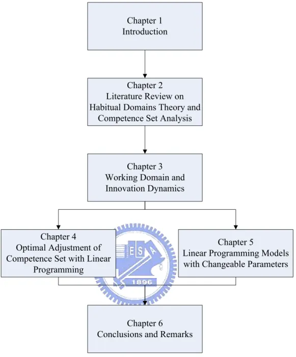
(17) than on the adjustment of the competence set to reach a target. We utilize multiple criteria and multiple constraint levels linear programming (MC2LP) model and its extended techniques to explore the linear programming models with changeable parameters. The parameters include: unit profit, available resources and input-output coefficients of production function. With those parameters changed with capital investment and/or time, we study how to find dynamic best solutions to make “taking loss at the ordering time and making profit at the time of delivery” feasible. For more general cases we also sketch a generalized mathematical programming model with changeable parameters and control variables. Chapter 6 concludes this work and proposes the future work. Finally, the references and appendices are attached at the end of the dissertation.. Figure 1-2 depicts the organization of the dissertation as follows.. -6-.

(18) Chapter 1 Introduction. Chapter 2 Literature Review on Habitual Domains Theory and Competence Set Analysis. Chapter 3 Working Domain and Innovation Dynamics. Chapter 4 Optimal Adjustment of Competence Set with Linear Programming. Chapter 5 Linear Programming Models with Changeable Parameters. Chapter 6 Conclusions and Remarks. Figure 1-2 The organization of the dissertation.. -7-.

(19) CHAPTER 2 LITERATURE REVIEW ON HABITUAL DOMAINS THEORY AND COMPETENCE SET ANALYSIS. In order to facilitate the latter discussion, we shall in this chapter introduce the habitual domains theory and the competence set analysis.. 2.1 Habitual Domains Theory Each person has a unique set of behavioral patterns resulting from his/her ways of thinking, judging, responding, and handling problems, which gradually stabilized within a certain boundary over a period of time (see Yu [11], [12], [13]). This collection of ways of thinking, judging, etc., accompanied with its formation, interaction, and dynamics, is called habitual domain (HD). Let us take a look at an example.. Example 2.1. Chairman Ingenuity. A retiring corporate chairman invited to his ranch two finalists, say A and B, from whom he would select his replacement using a horse race. A and B, equally skillful in horseback riding, were given a black and white horse respectively. The chairman laid out the course for the horse race and said, “Starting at the same time now, whoever’s horse is slower in completing the course will be selected as the next Chairman!” After a puzzling period, A jumped on B’s horse and rode as fast as he could to the finish line while leaving his horse behind. When B realized what was going on, it was too late! Naturally, A was the new Chairman.. Most people consider that the faster horse will be the winner in the horse race (a habitual. -8-.

(20) domain). When a problem is not in our HD, we are bewildered. The above example makes it clear that one’s habitual domain can be helpful in solving problems but it also can come his or her way of thinking. Moreover, one may be distorting information in a different way.. 2.1.1 Behavior Mechanism Habitual domain is very closely related to our life goals, behavior, and decision making. To understand habitual domains theory in advance, it is necessary to know how our wonderful brain and mind work. Yu [11], [12], [13] has tried to capture the behavior mechanism through eight basic hypotheses based on the findings and observations of psychology and neuron science. The eight hypotheses are listed in the Appendix 1.. The basic concept of the behavior mechanism is originated from the abilities of internal information process and problem solving. With the help of these abilities, we can perform variety of activities and handle diversity of events. The brain is the internal information process center. Our memory and thought processes are summarized according to four basic hypotheses: circuit pattern hypothesis, unlimited capacity hypothesis, efficient restructuring hypothesis, and analogy/association hypothesis. Understanding each hypothesis thoroughly is essential to understanding human behavior. The remaining four hypotheses are related to how our mind works: goal setting and state evaluation hypothesis, charge structures and attention allocation hypothesis, discharge hypothesis, and information input hypothesis.. Let us briefly state five aspects of the dynamics of behavior mechanisms as follows. These five aspects continuously interact with each other, resulting in infinite wonderful human behavior patterns.. 1.. Experience, learning and memory are the bases for interpreting and judging arriving. -9-.

(21) events;. 2.. The dynamics of unfavorable discrepancies, between the ideal goal states (or equilibriums) and the perceived states, create the dynamic change of charge structure, which commands attention allocation and prompts actions, passively or actively; (the charge, a kind of mental force, is a precursor to drive or stress.). 3.. Dynamic attention allocation, at any given point in time, to the events perceived as most significant (measured in terms of charges) is a fundamental element in human information processing;. 4.. The least resistance principle, which is the way that human beings release their charges, includes active problem solving or avoidance justification;. 5.. External information is necessary for human beings to achieve and maintain their ideal goals; unless attention is paid, the external information is not processed.. The above dynamics of human behavior can be depicted in Figure 2-1. The human brain. -10-.

(22) Problem Solving or Avoidance Justification. Physiological Monitoring. Unsolicited Information Solicited Information. Self-suggestion Figure 2-1 The behavior mechanism [11].. is the internal information-processing center, which receives all kinds of information from various sources. Each one of us has a set of living goals and for each living goal we have an ideal state or equilibrium point to reach and maintain (goal setting). Yu [12] classified living goals as a structure of goal functions comprised of seven goals which has shown in Table 2-1.. -11-.

(23) Table 2-1 A structure of goal functions [12]. (i). Survival and Security: physiological health (correct blood pressure, body temperature and balance of biochemical state); right level and quality of air, water, food, heat, clothes, shelter and mobility; safety; acquisition of money and other economic goods;. (ii) Perpetuation of the Species: sexual activities; giving birth to the next generation; family love; health and welfare; (iii) Feelings of Self-Importance: self-respect and self-esteem; esteem and respect from others; power and dominance; recognition and prestige; achievement; creativity; superiority; accumulation of money and wealth; giving and accepting sympathy and protectiveness; (iv) Sensuous Gratification: sexual; visual; auditory; smell; taste; tactile; (v) Cognitive Consistency and Curiosity: consistency in thinking and opinions; exploring and acquiring knowledge, truth, beauty and religion; (vi) Self-Actualization: ability to accept and depend on the self, to cease from identifying with others, to rely on one’s own standard, to aspire to the ego-ideal and to detach oneself from social demands and customs when desirable.. We continuously monitor, consciously or subconsciously, where we are relative to the ideal state or equilibrium point (state evaluation). Goal setting and state evaluation are dynamic, interactive and are subject to physiological forces, self-suggestion, external information forces, current memory and information processing capacity. When there is an unfavorable discrepancy of the perceived value from the ideal, each living goal will produce various levels of charge. The totality of the charges by all living goals is called the charge structure and it can change dynamically. At any point in time, our attention will be paid to the event which has the most influence on our charge structure. To release charges, we tend to -12-.

(24) select the action (which belongs to either active problem solving or avoidance justification) which yields the lowest remaining charge (the remaining charge is the resistance to the total discharge) and this is called the least resistance principle. When we try to relieve pains or frustrations, external information inputs may not be processed unless attention is paid.. 2.1.2 The Four Basic Elements of Habitual Domain Our habitual domains go wherever we go and have great impact on our decision making. As our HD, over a period of time, will gradually become stabilized, unless there is an occurrence of extraordinary events or we purposely try to expand it, our thinking and behavior will reach some kind of steady state and predictable. Our habitual domains are comprised of the following four elements.. 1.. Potential domain (PD). This is the collection of all thoughts, concepts, ideas, and actions that can be potentially activated by one person or by one organization. The potential domain at time t is denoted by PDt.. 2.. Actual domain (AD). This is the collection of all thoughts, concepts, ideas, and actions, which actually catch our attention and mind. The actual domain at time t is denoted by ADt.. 3.. Activation Probability (AP). This represents the probability that the ideas, concepts and actions in the potential domain that can be actually activated. The activation probability at time t is denoted by APt. Furthermore, we denote the activation probability of an idea i at time t by APt(i). That is, the activation probability of the ith element in the potential domain. Note that the activation probability of an idea will be strengthened by repeatedly activating the idea.. -13-.

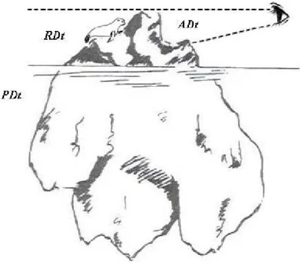
(25) 4.. Reachable domain (RD). This is the collection of thoughts, concepts, ideas, actions and operators that can be generated from initial actual domain. The reachable domain that generated from an idea set It and the operator set Ot at time t is denoted by RDt(It, Ot).. At any point in time habitual domains, denoted by HDt, will mean the collection of the above four subsets. That is, HDt = (PDt, ADt, APt, RDt(It, Ot)). In general, the actual domain is only a small portion of the reachable domain; in turn, the reachable domain is only a small portion of potential domain, and only a small portion of the actual domain is observable. That is, ADt ⊂ RDt(It, Ot) ⊂ PDt. Note that HDt changes with time. We will take an example to illustrate PDt, ADt, and RDt.. Example 2.2. Assume we are taking an iceberg scenic trip. At the moment of seeing an iceberg, we can merely see the small part of the iceberg which is above sea level and faces us. We cannot see the part of iceberg under sea level, nor see the seal behind the back of iceberg (see Figure 2-2). Let us assume t is the point of time when we see the iceberg, the portion which we actually see may be considered as the actual domain (ADt), in turn, the reachable domain (RDt) could be the part of iceberg above sea level including the seal. The potential domain (PDt) could be the whole of the iceberg including those under the sea level.. -14-.

(26) Figure 2-2 A vivid illustration of PDt, RDt, and ADt.. At time t, if we do not pay attention to the backside of the iceberg, we will never find the seal. In addition to this, never can we see the spectacular iceberg if we do not dive into the sea. Some people might argue it is nothing special to see a seal on the iceberg. But, what if it is a box of jewelry rather than a live seal! This example illustrates that the actual domain can easily get trapped in a small domain resulting from concentrating our attention on solving certain problems. In doing so, we might overlook the tremendous power of the reachable domain and potential domain.. 2.1.3 Degree of Habitual Domain Expansion In studying the expansion of habitual domains, we shall focus only on how we expand the actual domains (ADs) from its initial sets at an initial point of time, say s (starting time), to another time, t. Let ADst be the actual domain accumulated from s to t.. -15-.

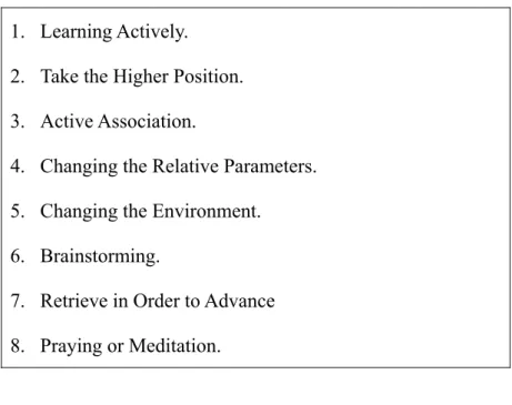
(27) There are three kinds of expansions of the actual domains as follows [12]:. 1.. Zero degree expansion. Starting from the original set ADs, one can expand the actual domains to a subset of the reachable domains. Mathematically speaking, ADst has a zero degree expansion if ADst \ ADs ≠∅ and RDs ⊃ ADst. Note, RDs is a function of ADs. There are no extraordinary events within the time interval [s, t] to trigger a new conception that is outside of the reachable domain RDs.. 2.. First degree expansion. By expansion of first degree, we mean that the actual domain ADst is not contained by the reachable domain RDt, but is still contained in the potential domain PDs. That is, ADst \ RDt ≠ ∅ and PDs ⊃ ADst.. 3.. Second degree expansion. By second degree expansion we mean that through external information inputs or self-suggestion we acquire new concepts or operators which are not contained by our previous potential domains. Therefore, the actual domain ADst is not contained by PDs. That is, ADst \ PDs ≠ ∅.. There are many methods for helping us to improve or expand our habitual domains and avoid decision traps. We list some of them in the following Table 2-2 and Table 2-3. In the Appendix 2 and 3, we briefly provide eight basic methods and nine principles for deep knowledge which are some mental operators (thinking procedure and attitudes). The interested reader is referred to [11], [12], and [13] for more detail. -16-.

(28) Table 2-2 Eight basic methods for expanding habitual domains. 1. Learning Actively. 2. Take the Higher Position. 3. Active Association. 4. Changing the Relative Parameters. 5. Changing the Environment. 6. Brainstorming. 7. Retrieve in Order to Advance 8. Praying or Meditation.. Table 2-3 Nine principles for deep knowledge. 1. Deep and Down Principle. 2. Alternating Principle. 3. Contrasting and Complementing Principle. 4. Revolving and Cycling Principle. 5. Inner Connection Principle. 6. Changing and Transforming Principle. 7. Contradiction Principle. 8. Cracking and Ripping Principle. 9. Void Principle.. 2.2 Competence Set Analysis For each decision problem or event E, there is a competence set consisting of ideas, knowledge, skills, and resources for its effective solution [8], [9]. When the decision maker. -17-.

(29) (DM) thinks he/she has already acquired and mastered the competence set as perceived, he/she would feel comfortable making the decision. Note that conceptually, competence set of a problem may be regarded as a projection of a habitual domain on the problem. Thus, it also has potential domain, actual domain, reachable domain, and activation probability as described in subsection 2.1.2. Also note that through training, education, and experience, competence set can be expanded and enriched (i.e. its number of elements can be increased and their corresponding activation probability can become larger).. 2.2.1 α-core Competence Set Given an event or a decision problem E which catches our attention at time t, the probability or propensity for an idea I or element in our habitual domains that can be activated is denoted by Pt(I, E). Like a conditional probability, we know that 0 ≤ Pt(I, E) ≤ 1, that Pt(I, E) = 0 if I is unrelated to E or I is not an element of Pt (potential domain) at time t; and that Pt(I, E) = 1 if I is automatically activated in the thinking process whenever E is presented. Empirically, like probability functions, Pt(I, E) may be estimated by determining its relative frequency. For instance, if I is activated 7 out of 10 times whenever E is presented, then Pt(I, E) may be estimated at 0.7. Probability theory and statistics can then be used to estimate Pt(I, E). The α-core of competence set at time t, denoted by Ct(α, E), is defined to be the collection of skills or elements of our habitual domains that can be activated with a propensity larger than or equal to α. That is, Ct(α, E)={I| Pt(I, E) ≥ α} as depicted in Figure 2-3 for illustration.. -18-.

(30) Figure 2-3 Illustration of α-core competence set [12].. 2.2.2 Four Elements of Competence Set For a given problem E there are four basic elements of competence set and they are interrelated as depicted in Figure 2-4.. 1.. The true competence set (Tr(E)): consists of ideas, knowledge, skills, attitudes, information and resources that are truly needed for solving problem E successfully;. 2.. The perceived competence set (Tr*(E)): The true competence set as perceived by the decision maker (DM);. 3.. The DM’s acquired skill set (Sk(E)): consists of ideas, knowledge, skills, attitudes, information and resources that have actually been acquired by the DM;. 4.. The perceived acquired skill set (Sk*(E)): The acquired skill set as perceived by the DM.. -19-.

(31) Tr(E) The True Competence Set. Ignorance, Uncertainty Illusion. Decision Quality. Sk(E) The Acquired Skill Set. Tr*(E) The Perceived Competence Set Confidence, Risk Taking. Illusion Ignorance, Uncertainty. Sk*(E) The Perceived Acquired Skill Set. Figure 2-4 Four basic elements of competence set and their relationships [12].. Note that the above four elements are some special subsets of the habitual domain (HD) of a decision problem E, see [11] for details. For simplicity and without confusion, we shall drop E for the following discussion. The four elements are closely related. For instance:. 1.. The gaps between the true competence set (Tr or Sk) and perceived competence set (Tr* or Sk*) are due to ignorance, uncertainty, illusion and wishful thinking;. 2.. If Tr* is much larger than Sk* (i.e. Tr*⊃⊃Sk*), the DM would feel uncomfortable and lack confidence to make decisions; conversely, if Sk* is much larger than Tr* (i.e. Sk*⊃⊃Tr*), the DM would be fully confident in making decisions;. 3.. If Sk is much larger than Sk* (i.e. Sk⊃⊃Sk*), the DM underestimates his own competence; conversely, if Sk* is much larger than Sk (i.e. Sk*⊃⊃Sk), the DM overestimates his own competence;. 4.. If Tr is much larger than Tr* (i.e. Tr⊃⊃Tr*), the DM underestimates the difficulty of the problem; conversely, if Tr* is much larger than Tr (i.e. Tr*⊃⊃Tr), the DM overestimates -20-.

(32) the difficulty of the problem;. 5.. If Tr is much larger than Sk (i.e. Tr⊃⊃Sk), and decision is based on Sk, then the decision can be expected to be of low quality; conversely, if Sk is much larger than Tr (i.e. Sk⊃⊃Tr), then the decision can be expected to be of high quality.. 2.2.3 Classification of Decision Problems Let the truly need competence set at time t, the acquired skill set at time t, and the α-core of an acquired skill set at time t be denoted by Trt(E), Skt(E), and Ct(α, E), respectively. Depending on Trt(E), Skt(E), and Ct(α, E), we may classify decision problems into following categories:. 1.. If Trt(E) is well-known and Trt(E)⊂Ct(α, E) with high value of α or α→1, as depicted in Figure 2-5, then the problem is a routine problem, for which satisfactory solutions are readily known and routinely used.. Figure 2-5 Routine problems.. 2.. Mixed-routine problem consists of a number of routine sub-problems, we may decompose it into a number of routine problems to be solved.. 3.. If Trt(E) is only fuzzily known, the ideas, concepts and skills are elements of the -21-.

(33) potential domain PDt, even if they may not contained in Ct(α, E) with a high value of α, as depicted in Figure 2-6, then the problem is a fuzzy problem, for which solutions are fuzzily known. Note that once the Trt(E) is gradually clarified and contained in α-core with a high value of α, the fuzzy problem may gradually become routine problem.. Figure 2-6 Trt(E) is only fuzzily known.. 4.. If Trt(E) \ Ct(α, E) is very large relative Ct(α, E) no matter how small is α or Trt(E) is unknown and difficult to know, which implies that Trt(E) contains some elements outside of the existing potential domain, as depicted in Figure 2-7. Then the problem is a challenging problem. Because of the fact that the most part of Trt(E) is unknown and there are many parameters, which can vary over certain ranges or domains, challenging decision problems are very complex. Yu and Chianglin (2006) described this kind of problems as decision problems with changeable spaces (parameters). A system scheme based on HDs theory has been introduced to help us reduce decision blinds and avoid decision traps so that we could make quality decisions.. -22-.

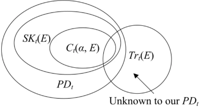
(34) SKt(E). Ct(α, E). Trt(E). PDt Unknown to our PDt. Figure 2-7 Competence set of challenging problems.. -23-.

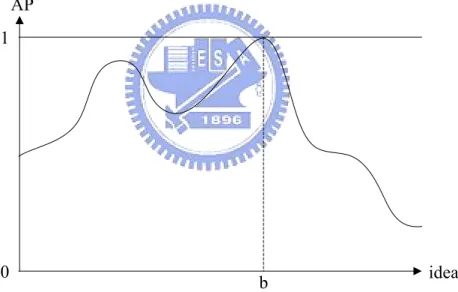
(35) CHAPTER 3 WORKING DOMAIN AND INNOVATION DYNAMICS. Based on HD theory and CS analysis, we shall in this chapter introduce the concepts of working domain and innovation dynamics. We could see how our working domains can commit decision traps and how to avoid them. The model of innovation dynamics helps our working domains become more flexible and agile.. 3.1 Property of the Activation Probability In order to facilitate the later discussion, we shall introduce the activation continuity assumption [14]: let s and t be two distinct point of time, i.e., s≠t, all activated ideas and operators for solving a given decision problem can be continuously activated again within the time interval [s, t] if needed. In general, the activation continuity assumption is held when either of the following two cases occurs:. 1.. the time interval [s, t] is sufficiently small;. 2.. all the activated ideas, concepts, and information for solving the decision problem can be properly recorded and saved.. If the activation continuity assumption does not hold, let t1, t2, t3∈[s, t] and s<t1<t2<t3<t. Suppose that the activation probability for each circuit pattern at t1, t2, and t3, denoted by APt1 ,. APt2 , and APt3 , is shown in Figure 3-1, 3-2, and 3-3, where the actual domains with respect to t1, t2, and t3 are ADt1 = {a} , ADt2 = {b} , and ADt3 = {c} respectively. -24-.

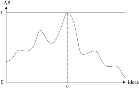
(36) Figure 3-1 The activation probability for circuit patterns at t1.. AP 1. 0. b. ideas. Figure 3-2 The activation probability for circuit patterns at t2.. -25-.

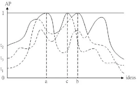
(37) AP 1. 0. ideas. c. Figure 3-3 The activation probability for circuit patterns at t3.. Suppose that the time interval [s, t] is sufficiently small (i.e., the activation continuity assumption is held). Figure 3-4 depicts the activation probability for circuit patterns at t3. The corresponding actual domain is then ADt3 = {a, b, c} since all the activated ideas and operators could be retrieved if needed. By the activation continuity assumption, the activation probability for each circuit pattern at time t2 and t3 can be denoted by. {. }. APt2 ( i ) = max APt1 ( i ) , APt2 ( i ) ,. (1). and. {. }. APt3 ( i ) = max APt1 ( i ) , APt2 ( i ) , APt3 ( i ) .. (2). For generalization, let t0 be the time that we encounter a decision problem. The activation probability for an idea i at time tnow ≥ t0 can be denoted by APtnow ( i ) = max. {t0 ≤ t ≤ tnow }. -26-. { AP ( i )} . t.

(38) Figure 3-4 The activation probability for circuit patterns at t3 when the activation continuity assumption is held.. By (1), (2) and Figure 3-4, if the activation continuity assumption is held, the activation probability would be increased when time passes. On the other hand, the ideas and operators in our brains would be increased and more easily to be retrieved when time passes. Therefore, how to make the activation continuity assumption be held is very important for solving a decision problem.. 3.2 Working Domain The memory of humanity is one of extensive research issues studied by psychologists. A number of classifications and models related to the memory are introduced. Working memory (WM) plays a vital role in our life especially when cognitive works such as learning, comprehending, and reasoning etc. [16], [17] are performed. WM will be used when we try to look up a telephone number and remember it to dial it without writing it down [18], [19]. Atkinson and Shiffrin [20], [21] proposed that short-term memory works as WM which allows us to retain useful information as to solve the problem to use it. Olton et al. [22], [23] -27-.

(39) proposed that WM is a system which is responsible for the maintenance of the information related to the works we have to do so that we could perform efficiently.. Baddeley and Hitch [24] gave the definition of WM which is a system used to temporarily store and manipulate information to help us in complicated cognitive work and developed the multiple-component model of WM, as shown in Figure 3-5.. Phonological Loop. Central Executive. VisuoSpatial Sketchpad. Long-term Memory. Figure 3-5 Multiple-component model of working memory [24].. The model consisted of two slave systems (phonological loop and visuo-spatial sketchpad) and a central executive. The former are responsible for short-term maintenance of information, and the latter is responsible for the supervision of information integration and for coordinating the slave systems. Subsequently, Baddeley [25] added episodic buffer, a fourth component, to the model. The episodic buffer is the third slave system which is responsible for linking information across domains to form integrated units of visual, spatial, and verbal information with time sequencing (or chronological ordering), such as the memory of a story. -28-.

(40) Based on habitual domains theory, working domain (WD) refers to the set of all the ideas and the operators used to relieve our charge structure, which is inflicted by a decision problem. For example, when sharing the knowledge about the breeding of dogs, all the related special experiences, such as the name, the figure, and the barks of the dog, will be retrieved. Hence, we may portray the WD as the set of ideas which has been actually activated for solving the decision problem or the set of ideas whose activation probabilities are greater than α (0≤α≤1). The former is denoted by. WD ( E ) = {i ∈ HDt | APt (i ) = 1, ∀t ∈ [t1 , t2 ]} ,. (3). and the latter is denoted by. WDα ( E ) = {i ∈ HDt | APt (i )≧ α, ∀t ∈ [t1 , t2 ]} ,. (4). where i denotes an idea; APt(i) denotes the activation probability of the idea i at time t, t1 is the point of time when a decision problem is constituted, and t2 is the point of time when the decision problem is solved.. Note that the actual domains are emphasized in (3), and both the actual domains and the reachable domains are included in (4).. 3.3 Classification of Decision Problems Let the needed competence set, the potential domain, and the working domain with respect to a given decision problem or event E at time t are denoted by CSt(E), PDt(E), and WDt(α, E), respectively. We may restate the four categories mentioned in subsection 2.2.2 into the following:. 1.. If CSt(E) is well-known and CSt(E)⊂WDt(α, E)⊂PDt(E), α→1, then the problem is a -29-.

(41) routine problem. When encounter this class of problems, we know the truly needed competence set without ambiguous so that the problem could be efficiently solved. That is, our working domain can immediately react to solve it.. 2.. Mixed-routine problem consists of a number of routine sub-problems, we may decompose it into a number of routine problems to be solved.. 3.. If CSt(E) is only fuzzily known and may not contained in WDt(α, E) with a high value of α, then the problem is a fuzzy problem, for which solutions are fuzzily known. That is, CSt(E)\WDt(α, E)≠∅, and CSt(E)⊂PDt(E). Note that once the CSt(E) is gradually clarified and contained in α-core with a high value of α, the fuzzy problem may gradually become routine problem.. 4.. If CSt(E) is unknown or a small part of CSt(E) is known and the remaining part is not in PDt(E), then the problem is a challenge problem. That is, CSt(E)\WDt(α, E)≠∅, and CSt(E)\PDt(E)≠∅. Note that no matter how low the degree of α is, CSt(E) can not be included by WDt(α, E).. These four decision problems can be easily seen in our life. Information technologies (ITs) only can facilitate us to solving routine problems and mixed-routine problems other than challenge problems due to the unknown CSt(E). Even if a small part of CSt(E) is known, the remaining part is not in our habitual domains. Let us see the following example.. Example 3.1. Adopted from [26]. Archimedes, a great scientist, was summoned by the. King of Greece to verify if his new crown was made of pure gold. Of course, in the verification process, the beautiful crown should not be damaged. The problem was a great challenge and created a very high level of charge on Archimedes. The scientist’s curiosity was. -30-.

(42) increased and his reputation was at stake. The burning desire to solve the problem kept Archimedes awake day and night. One day, when Archimedes was in his bathtub watching the water fill up and overflow, a solution suddenly struck him. He rushed out of the bathtub shouting “eureka” (means “I found it” in Greek) and in his excitement, he even forgot to put on his clothes. His discovery which is the well-known displacement principle states that the volume of the displaced water should be equal to the volume of his entire body in the water. Thus the crown, when immersed in the water, should displace its own volume. By comparing the weight of the crown with an equivalent weight of pure gold of the same volume, one should be able to verify if the crown is made of pure gold. What a relief to Archimedes!. The problem whether the new crown of the King of Greece was made of pure gold without damage is a challenge problem to Archimedes. When Archimedes was taking a bath (routine problem) in his bathtub, he noticed the water fill up and overflow (information input). His working domain was expanded through active association so that he came up with a simple but great solution for verifying if the new crown was made of pure gold.. 3.4 How Working Domain Get Trapped With rapid advancement of Information Technology (IT), Knowledge Management (KM) has enjoyed its rapid growth [27]. In the market, there are many software available to help people make decisions or transactions, such as supply chain management (SCM), enterprise resource planning (ERP), customer relationship management (CRM), accounting information system (AIS), etc. [28], [29], [30]. In the nutshell, KM is useful because it can help certain people to relieve the pains and frustrations for obtaining useful information to make certain decisions or transactions. For salesperson, KM could provide useful information as to close sales. For credit card companies, KM could provide useful information about card holders’. -31-.

(43) credibility. For supply chain management, KM can efficiently provide where to get needed materials, where to produce and how to transport the product and manage the cash flow, etc.. It seems, KM could do “almost everything” to help people make “any decision” with good results. Let us consider the following example.. Example 3.2. Breeding Mighty Horses. For centuries, many biologists paid their. attention and worked hard to breed endurable mighty working horses so that the new horse could be durable, controllable and did not have to eat. To their great surprise, their dream was realized by mechanists, who invented a kind of “working horse”, tractors. The biologists’ decision trap and decision blind are obvious.. Biologists habitually thought that to produce the mighty horses, they had to use ”breeding methods”−a bio-tech, a decision trap in their mind. Certainly, they made progress. However, their dream could not be realized.. IT or KM, to certain degree, is similar to breeding, a biotech. One wonders: is it possible that IT or KM could create traps for people as to make wrong decision or transactions? If it is possible, how could we design a good KM that can minimize the possibility to have decision traps and maximize the benefits for the people who use it?. In the information era, even the advances of IT and KM can help solve people’s decision problems, our working domain could still easily get trapped, leading us to make wrong decision or action.. Example 3.3. Dog Food. A dog food company designed a special package that not only. was nutritious, but also could reduce dogs’ weight. The statistical testing market was positive. The company started “mass production”. Its dog food supply was far short from meeting the -32-.

(44) overwhelming demand. Therefore, the company doubled its capacity. To their big surprise, after one to two months of excellent sales, the customers and the wholesalers began to return the dog food package, because the dogs did not like to eat it.. Clearly, a decision trap was committed by using statistics on buyers, not on the final users (dogs). The KM used statistical method on “wrong” subject and committed the trap. If the RD (reachable domain) of the KM could include the buyers and the users, the decision traps and wrong decisions might be avoided.. So far, KM with IT can accelerate decisions for the routine or mixed-routine problems. There still are many challenging problems, which cannot be easily solved by KM with IT. This is because the needed competence set (Trt(E)) of a challenging problem is unknown or only partially known, especially when humans are involved. The following illustrates this fact.. Example 3.4. Alinsky’s Strategy. Adapted from [31]. In 1960 African Americans living. in Chicago had little political power and were subject to discriminatory treatment in just about every aspect of their lives. Leaders of the black community invited Alinsky, a great social movement leader, to participate in their effort. Alinsky clearly was aware of deep knowledge principles. Working with black leaders he came up with a strategy so alien to city leaders that they would be powerless to anticipate it. He would mobilize a large number of people to legally occupy all the public restrooms of the O’Hare Airport. Imagine thousands of individuals visit the airport daily who were hydraulically loaded (very high level of charge) rushed for restroom but there would be no place for all these persons to relieve themselves.. How embarrassing when the newspaper and media around the world headlined and dramatized the situation. As it turned, the plan never was put into operation. City authorities -33-.

(45) found out about Alinsky’s strategy and, realizing their inability to prevent its implementation and its potential for damaging the city’s reputation, met with black leaders and promised to fulfill several of their key demands.. The above example shows us the importance of understanding one’s potential domain. At the beginning, African Americans did not entirely know the habitual domain of city authorities (a challenging problem). Their campaigns, such as demonstration, hunger strike, etc., failed to reach their goal (an working domain). Alinsky observed a potentially high level of charge of the city authorities, the public opinion (potential domain), that could force them to act. As a result, the authorities agreed to meet the key demands of the black community, with both sides claiming a victory.. 3.5 Innovation Dynamics Without creative ideas and innovation, our lives will be bound in a certain domain and become stable. Similarly, without continuous innovation, our business will lose its vitality and competitive edge [32], [33]. Bill Gates indicated that Microsoft would collapse in about two years if they do not continue the innovation.. In this section, we are going to explore innovation dynamics based on Habitual Domains (HD) and Competence Set (CS) Analysis as to increase competitive edge. From HD theory and CS analysis, all things and humans can release pains and frustrations for certain group of people at certain situations and time. Thus all humans and things carry the competence (in broad sense, including skills, attitudes, resources, and functionalities). For instance, a cup is useful when we need a container to carry water as to release our pains and frustrations of having no cup.. -34-.

(46) The competitive edge of an organization or human can be defined as the capability to provide right services and products at right price to the target customers earlier than the competitors, as to release their pains and frustrations and make them satisfied and happy.. To be competitive, we therefore need to know what would be the customers’ needs as to produce the right products or services at a lower cost and faster than the competitors. At the same time, given a product or service of certain competence or functionality, how to reach out the potential customers as to create value (the value is usually positively related to how much we could release the customers’ pains and frustrations).. If we abstractly regard all humans and things as a set of different CS, then producing new products or services can be regarded as a transformation of the existent CS to a new form of CS. Based on this, we could draw clockwise innovation dynamics as in Figure 3-6:. -35-.

(47) Figure 3-6 Clockwise Innovation Dynamics.. Although Figure 3-6 is self-explaining, the following are worth mentioning. The numbers are corresponding to that of the figure.. Note 1: According to HD Theory, when the current states and the ideal goals have unfavorable discrepancies (for instance losing money instead of making money, technologically behind, instead of ahead of, the competitors), these discrepancies will create mental charge which can prompt us to work harder to reach our ideal goals.. Note 2: Producing product and service is a matter of transforming CS from the existing one to -36-.

(48) a new form.. Note 3: Our product could release the charges and pains of certain group of people and make them satisfied and happy.. Note 4: The organization can create or release charges of certain group of people through advertising, marketing and selling.. Note 5: The target group of people will experience the change of charges. When their pains and frustrations, by buying our products or services, are relieved and become happy, the products and services can create value, which is Note 6.. Note 7 and Note 8 respectively are the distribution of the created value and reinvestment. To gain the competitive edge, products and services need to be continuously upgraded and changed. The reinvestment, Note 8, is needed for research and development for producing new product and service.. In a contrast, the innovation dynamics can be counter-clockwise. We could draw counter-clockwise innovation dynamics as in Figure 3-7:. -37-.

(49) Figure 3-7 Counter-clockwise Innovation Dynamics.. Note 1: According to HD Theory, when the current states and the ideal goals have unfavorable discrepancies will create mental charge which can prompt us to work harder to reach our ideal goals.. Note 2: In order to make profit, organization must create value.. Note 3: According to CS analysis, all things carry competence which can release pains and frustrations for certain group of people at certain situations and time.. Note 4: New business opportunities could be found by understanding and analyzing the pains and frustrations of certain group of people.. Note 5: Reallocation or expansion of competence set is needed for innovating products or. -38-.

(50) services to release people’s pains and frustrations.. Innovation needs creative ideas, which are outside the existing HD and must be able to relieve the pains and frustrations of certain people. From this point of view, the method of expanding and upgrading our HDs becomes readily applicable. Innovation can be defined as the work and process to transform the creative ideas into reality as to create the value expected. It includes planning, executing (building structures, organization, processes, etc.), and adjustment. It could demand hard working, perseverance, persistence and competences. Innovation is, therefore, a process of transforming the existing CS toward a desired CS (product or service).. -39-.

(51) CHAPTER 4 OPTIMAL ADJUSTMENT OF COMPETENCE SET WITH LINEAR PROGRAMMING. The innovation dynamics could be portrayed as a process of transforming the existent competence set to a new form of competence set. It includes planning, executing (building structures, organization, processes, etc.), and adjustment. After having known the innovation dynamics, we shall in this chapter focus on the optimal adjustment of competence set so that an expected state could be achieved. To make our studies specific and mathematically precise we shall limit ourselves to linear models based on management by objectives (MBO).. 4.1 Introduction to Optimal Competence Set Adjustment Problems MBO is an efficient and effective managerial system [34]. Goal setting is the first crucial step in the system of MBO. At this step the participants identify the targets to be achieved. The company then mobilizes all resources and competence, including their reallocation, to reach the targets, or to move toward the targets as close as possible. Therefore, achieving the targets becomes one of the most important criteria in the system of MBO. In order to achieve the targets some relevant parameters, such as the constraint coefficients and the right hand sided resource level in linear programming (LP) problems, need to be adjusted and/or expanded.. One of the well-known researches on the adjustment of parameters is the inverse LP optimization. In the class of inverse LP problems, the parameters of the objective function. -40-.

(52) with the minimum deviation from the original ones are sought so that a given feasible solution x′ becomes an optimal one [35]. Zhang and Liu [36] studied inverse assignment and. minimum cost flow problems under L1-norm based on optimality conditions for LP problems. Zhang and Liu [37] further took L∞-norm into account and investigated inverse 0-1 programming and network programming problems. Ahuja and Orlin [38] considered more general inverse LP problems under both L1- and L∞-norms. In addition, Troutt et al. [39] investigated a so-called linear programming system identification problem in which both objective function coefficients and constraint matrix are evaluated to best fit a set of historical decisions and its corresponding used resources.. A competence set is a collection of ideas, knowledge, information, resources, and skills for satisfactorily solving a given decision problem [11], [12]. By using mathematical programming, a number of researchers have focused on searching for the optimal expansion process from an already acquired competence set to a needed one [9], [40], [41]. Feng and Yu [42] proposed a minimum spanning table algorithm to find the optimal competence set expansion process without formulating the related mathematical program. However, the competence set so far has been assumed to be discrete and finite so as to represent its elements by nodes of a graph. This makes the applications of the competence set expansion in these studies somehow limited, because the number of feasible solutions of a linear system might not be discrete and finite.. In this chapter, we focus on linear systems. While the literature on inverse LP optimization treats only a feasible target, we intend to determine the optimal adjustment of constraint coefficients in a linear system so that a given target, originally unattainable, can be achieved. Given a target solution, we set up a competence set adjustment model (CSA model) to study the optimal adjustment of the related competence sets. The model will enable us to. -41-.

(53) find the optimal adjustment whenever the target is reachable.. In case the target is unattainable, we utilize the bisection method or the fuzzy linear programming techniques to help the DM revise the target as to make it an achievable one. The former is to find a solution which is as close as possible to the target and the latter is to interactively select an achievable target. Then the optimal adjustment could be derived from the aforementioned CSA model with the revised target.. 4.2 Problem Statement Consider a standard LP model as follows. max s.t.. z ( x ) = cx Ax ≤ b,. (5). x ≥ 0,. where c=[ci] is the 1×n objective coefficient vector, x=[xj] denotes the n×1 decision vector, A=[aij] is the m×n consumption (or productivity) matrix, and b=[bi] is the m×1 resource. availability vector. The sensitivity analysis helps us to investigate whether the optimal basis changes if ci, aij, or bi has been changed. It provides us insight into the ranges over which the parameters of a model can vary without changing the optimal basis. While the sensitivity analysis considers the changes on ci, aij, or bi, we consider the simultaneous changes on aij and bi so that a given target can be reached. Suppose that x0 is a target solution set by decision maker (DM). Let D be a parameter matrix whose element, δij, denotes the deviation from aij, and γ be a parameter vector whose component, γi, denotes the deviation from bi. By changing D and γ, we tried to construct X0(D,γ), where X0(D,γ)={x|(A+D)x≤b+γ}.. -42-.

(54) Since aij=0 implies that the resource i has no impact on the product j. Thus, aij is not subject to adjustment. Consequently, we have δij=0 if aij=0. Definition 4.1. Given a target x0, a feasible adjustment is a pair (D,γ) such that. (A+D)x0≤b+γ. Thus, x0∈X0(D,γ). Let Ψ={(D,γ)|x0∈ X0(D,γ)} be the set of all feasible adjustments, and Φ={(i,j)|aij≠0}, Definition 4.2. Given a target solution x0, and (D0, γ0)∈Ψ, define the relative adjustment. measure of (D0, γ0) by. ℜ( D 0 , γ 0 ) =. ∑. ( i , j )∈Φ. m. rij ( D 0 ) + ∑ si (γ 0 ) , i =1. where rij ( D 0 ) = | δ ij0 | | aij | , aij≠0,. and si(γ0)= | γ i0 | / hi ,. where ⎧| bi | if bi ≠ 0, hi = ⎨ ⎩| M i | if bi = 0.. Note that rij(D0), aij≠0, is a relative adjustment measure with respect to the parameter aij, while si(γ0) is that with respect to bi. Note, when bi=0, | γ i0 | / | bi | is not defined. The positive number Mi needs to be chosen properly to reflect the impact of the adjustment on bi. Remark 4.1. When needed, ℜ(D0, γ0), rij and si can be changed into other forms of cost. functions to fit the cost of adjustment.. -43-.

(55) Definition 4.3. A feasible adjustment alternative (D*, γ*) is optimal if (D*, γ*) minimizes. the relative adjustment measure over Ψ. That is, ℜ(D*, γ*) = min{ℜ(D, γ) | (D, γ)∈Ψ}.. The adjustment deviation measure as defined in Definition 4.2 is not a linear form because of “absolute value”. To eliminate the sign of the absolute value in Definition 4.2, the following Lemma 4.1 is useful.. Lemma 4.1. Given D=[δij] and γ=[γi], let aij =aij+δij and bi =bi+γi. Define D + = [δ ij+ ] , D − = [δ ij− ] , γ + = (γ 1+ ,… , γ m+ ) , and γ − = (γ 1− ,… , γ m− ) with. ⎧aij − aij ⎩ 0 ⎧a − a δ ij− = ⎨ ij ij ⎩ 0. δ ij+ = ⎨. ⎧bi − bi. γ i+ = ⎨. ⎩ 0. if aij > aij , otherwise; if aij > aij , otherwise; if bi > bi , otherwise;. ⎧bi − bi. if bi > bi ,. ⎩ 0. otherwise.. γ i− = ⎨ Then:. (i) δ ij = δ ij+ − δ ij− and γ i = γ i+ − γ i− , or D = D + − D − and γ = γ + − γ − . (ii) δ ij = δ ij+ + δ ij− and γ i = γ i+ + γ i− . (iii) δ ij+ , δ ij− , γ i+ , γ i− ≥ 0.. Proof.. -44-. (6) (7). (8). (9).

(56) (i) Since aij =aij+δij, we have δ ij = aij − aij . We may replace (7) by (10) as follows. if aij > aij ,. ⎧. 0 ⎩aij − aij. δ ij− = ⎨. otherwise.. (10). By subtracting (10) from (6) on both sides, we have ⎧ aij − aij. if aij > aij ,. δ ij+ − δ ij− = ⎨ ⎩ aij − aij. otherwise.. (11). By (11), we have δ ij = δ ij+ − δ ij− . That γ i = γ i+ − γ i− could be proved in a similar way.. (ii) By definition, ⎧ δ ij ⎩−δ ij. δ ij = ⎨. if δ ij > 0, otherwise.. (12). We may rewrite (12) as follows. ⎧ aij − aij. δ ij = ⎨ ⎩ aij − aij. if aij > aij , otherwise.. (13). Observe that (13) could be obtained by adding (10) to (6). Thus, | δ ij |= δ ij+ + δ ij− . That | γ i |= γ i+ + γ i− can be proved similarly.. (iii) It is obviously from (6)-(9).. □. Note that δ ij+ is the value of aij exceeding aij and δ ij− is that of aij below aij, while. γ i+ is the value of bi exceeding bi and γ i+ is that of bi below bi.. 4.3 Optimal Adjustment of Competence Set Given a target x0, we try to identify the optimal adjustment alternative (D*, γ*) by -45-.