國 立 交 通 大 學
電子工程學系 電子研究所碩士班
碩 士 論 文
頻寬-位元率-失真最佳化之移動估測
Bandwidth-Rate-Distortion Optimized Motion Estimation
研 究 生: 戴瑋呈
指導教授: 張添烜
頻寬-位元率-失真之移動估測
Bandwidth-Rate-Distortion Optimized Motion Estimation
研 究 生: 戴瑋呈 Student : Wei-Cheng Tai 指導教授: 張添烜 博士 Advisor: Tian-Sheuan Chang
國 立 交 通 大 學 電子工程學系 電子研究所碩士班
碩 士 論 文
A Thesis
Submitted to Department of Electronics Engineering & Institute of Electronics College of Electrical and Computer Engineering
National Chiao Tung University in Partial Fulfillment of Requirements
for the Degree of Master In
Electronics Engineering September 2008
Hsinchu, Taiwan, Republic of China
I
頻寬-位元率-失真最佳化之移動估測
研究生: 戴瑋呈 指導教授: 張添烜 博士 國立交通大學電子研究所碩士班 摘 要 移動估測在 H.264 視訊編碼的過程中,具有龐大的運算量和記憶體需求,然而 傳統的移動估測只考慮位元率和失真,未將記憶體頻寬納入考量,因此,在頻寬受 限的情形下,位元率和失真並未做到最佳化。為了解決以上因素,在此本論文提出 一個頻寬-位元率-失真最佳化的移動估測演算法,首先,我們提出一個頻寬-位元 率-失真最佳化的模型,藉由設立一個合理的搜尋範圍,在允許的頻寬下提升位元 率和失真的最大效能。其次,我們提出兩個方法來進一步提高前者模型的效能,一 種方法為隨內容感測的跳躍預測演算法,藉由跳躍預測所節省的頻寬來提升其餘複 雜畫面的編碼品質;另一方法為搜尋範圍邊界預測演算法,藉由設立一個適宜的搜 尋範圍邊界而對搜尋範圍作進一步的修正。相較於之前的研究,對於靜態畫面影像, 我們的設計在相同位元率與失真,以及平均搜尋範圍為 16 的情形下,頻寬可節省 70%,若加上跳躍預測演算法,則頻寬可節省 84%;對於動態畫面影像,我們的設 計在低頻寬的環境下,位元率可降低 13%,同時峰值信噪比也可提升 0.1dB。總結 我們的設計對於不同的頻寬環境變化下,不僅維持了效能,甚至更進一步提升了效 能,這顯現出我們的設計可適用於改進移動估測的處理。III
Bandwidth-Rate-Distortion Optimized Motion Estimation
Student: Wei-Cheng Tai Advisor: Tian-Sheuan Chang
Institute of Electronics National Chiao Tung University
Abstract
Motion estimation (ME) processing is the most computational and memory intensive component in H.264 encoder. However, traditional ME algorithms focus on rate and distortion performance and thus do not take memory bandwidth into consideration. Therefore, the rate and distortion performance are not optimized under bandwidth constraint. In this thesis, we propose bandwidth-rate-distortion (B-R-D) optimized ME algorithm to solve the issue mentioned above. First, we mainly propose a B-R-D optimized modeling method to determine an appropriate search range (SR) for maximizing rate distortion efficiency while can dynamically meet the available bandwidth. Then, we propose two methods, skip mode detection with content-aware scheme and SR boundary prediction method, to enhance the performance of B-R-D optimized modeling method. The skip mode detection with content-aware scheme is presented to save the most memory bandwidth and thus gives other complex MBs more bandwidth for better quality, and the SR boundary prediction method is presented to determine a feasible SR boundary for SR refinement. Compared with reference software [3], when coding in low motion sequence, the simulation result shows the proposed BRD design could improve the bandwidth saving up to 70% with almost the same performance at bit rate and PSNR under average search range size 16, and up to 84% with negligible PSNR degradation with skip design added; while coding in high motion sequence, the simulation result shows our design could save average bit rate up to 13% and at the same time increase average PSNR up to 0.1dB under low bandwidth constraint. In summary, our design could achieve the same and sometimes even better performance under various bandwidth constraints and thus it is suitable for improving ME process.
V
誌 謝
在交大的兩年時光裡,經歷了許多研究的困難,能夠順利地得到這個學位,得 感謝許多人的幫助。首先,要感謝我的指導教授—張添烜博士,這兩年來給我的支 持與鼓勵,無論在研究或生活上,每當遇到問題總是能給予我建議與協助,亦師亦 友般地訓練自己獨立思考的能力,讓我克服難關,順利地完成學業。另外,我也要 感謝我的口試委員們,交大資工彭文孝教授和清華電機陳永昌教授,感謝你們百忙 中抽空指導我,你們的寶貴意見使我獲益良多,讓我的論文更加完備。 感謝 VSP 實驗室的好夥伴們,特別感謝引我入門的林佑昆學長,帶領我一步 一步的做好研究,不厭其煩的給予指導,使我順利的完成研究。謝謝張彥中、李國 龍、李得瑋、郭子筠、林嘉俊、吳秈璟、廖英澤學長,教導我 IC 設計與 H.264 編 碼的觀念與技巧。再來要感謝曾宇晟、蔡宗憲、詹景竹同學,和你們一同討論研究、 嬉鬧彼此的過程,是一段很難忘的回憶。還有感謝張瑋城同學,從大學至今的相互 砥礪,一起在研究室或寢室熬夜趕研究,是一段很珍貴的日子。另外感謝實驗室的 學弟妹們:黃筱珊、許博淵、沈孟維、蔡政君、陳之悠、廖元歆,活潑的你們,使 我的研究生涯充滿歡樂。還要謝謝呂進德、李韋磬,和你們一同聊天運動,是我減 輕壓力的最好方式。 謝謝我的女友,無論任何時刻,總是在第一時間傾聽我、包容我,一同分享我 的喜怒哀樂,有時假日更陪著我在實驗室裡奮鬥,滿滿的感動溢於言表,沒有妳的 支持與鼓勵,就不會有成為碩士生的我。 最後要感謝支持我的家人們,我的爸媽和兩個弟弟們,在電話的另一端給予我 愛的鼓勵,你們的溫暖是我努力的最大支柱。 在此,僅將本論文獻給所有愛我與所有我愛的人。VII
C
C
o
o
n
n
t
t
e
e
n
n
t
t
1. Introduction ... 1
1.1. Background ... 1
1.2. Motivation and contribution ... 2
1.3. Thesis organization ... 2
2. Overview of environment-aware motion estimation algorithms ... 3
2.1. Overview of variable block-based motion estimation ... 3
2.2. Review of adaptive search range motion estimation ... 5
2.3. Review of power-aware motion estimation ... 6
2.4. Review of computation-aware motion estimation ... 7
2.5. Review of skip mode detection algorithm ... 8
2.5.1. Lagrangian cost motion estimation ... 9
2.5.2. All zero DCT blocks detection ... 9
3. Proposed B-R-D optimized motion estimation algorithm ... 11
3.1. Introduction ... 12
3.2. Proposed skip mode detection with content-aware scheme ... 13
3.2.1. Review of SAD-4x4-block threshold... 13
3.2.2. Refinement of SAD-4x4-block threshold ... 15
3.3. Proposed B-R-D optimized modeling method ... 16
3.4. SR boundary prediction method ... 24
3.5. Summary ... 25
4. Simulation and Analysis ... 27
4.1. BW pattern setting ... 27
4.2. Experimental result ... 29
VIII
4.2.2. The distribution of MB for skip mode analysis ... 46
4.2.3. Timing comparison with skip detection ... 48
4.2.4. Completion time comparison of BW random patterns ... 49
4.3. Summary ... 51
5. Hardware implementation ... 53
5.1. Hardware design ... 53
5.2. Implementation result ... 54
6. Conclusion and future work ... 55
6.1. Conclusion ... 55
6.2. Future work ... 56
7. Reference ... 57
IX
L
L
i
i
s
s
t
t
o
o
f
f
F
F
i
i
g
g
u
u
r
r
e
e
Fig. 2-1 (a)The mode hierarchy and (b) its block size for H.264 ... 4
Fig. 2-2 Different modes for H.264 motion estimation ... 4
Fig. 2-3 Search range prediction using neighboring vectors ... 5
Fig. 2-4 Power aware multimedia systems [8]... 7
Fig. 3-1 The total BRD optimized motion estimation algorithm flow ... 12
Fig. 3-2 Skip mode detection flow ... 13
Fig. 3-3 The trend between boundary and SAD (Normalized to Akiyo) ... 15
Fig. 3-4 (a) SAD and SAD-4x4-block threshold under different QP Threshold estimation under (b) QP20 (c) QP24 (d) QP28 (e) QP32 (f) QP36 .. 16
Fig. 3-5 B-R-D optimized modeling method flow ... 17
Fig. 3-6 Illustration of BW budget ... 17
Fig. 3-7 Illustration of BW prediction ... 20
Fig. 3-8 Illustration of bandwidth boundary determination ... 20
Fig. 3-9 Illustration of SR decision ... 22
Fig. 3-10 Illustration of SR modification ... 23
Fig. 3-11(a) Search range boundary predicted method flow ... 24
Fig. 4-1 6 kind of BW patterns: (a) SR constant 8 (b) SR constant 16 (c) SR constant 24 (d) SR random 8 (e) SR random 16 (f) SR random 24 ... 28
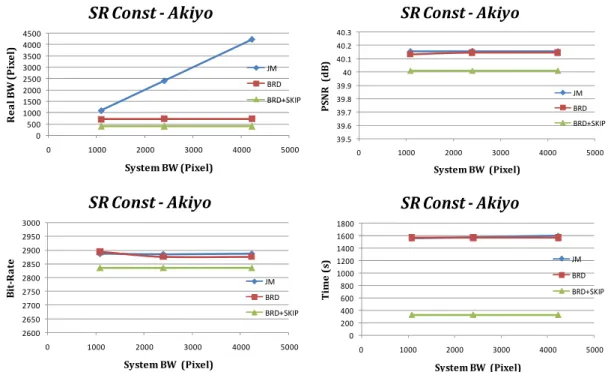
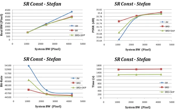
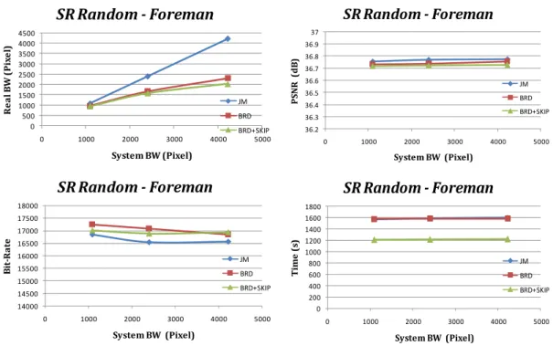
Fig. 4-2 The example of dynamically adjust the SR (a) The performance example of dynamiclly adjust the SR: (b) PSNR (c) Bit-rate . 29 Fig. 4-3 Performance comparison in (a) BW (b) PSNR (c)Bit-rate (d) Time ... 34
Fig. 4-4 Performance comparison in (a) BW (b) PSNR (c)Bit-rate (d) Time ... 34
Fig. 4-5 Performance comparison in (a) BW (b) PSNR (c)Bit-rate (d) Time ... 35
Fig. 4-6 Performance comparison in (a) BW (b) PSNR (c)Bit-rate (d) Time ... 35
Fig. 4-7 Performance comparison in (a) BW (b) PSNR (c)Bit-rate (d) Time ... 36
Fig. 4-8 Performance comparison in (a) BW (b) PSNR (c)Bit-rate (d) Time ... 36
Fig. 4-9 RD curve comparison under SR constant 8 for “Akiyo” sequence ... 40
X
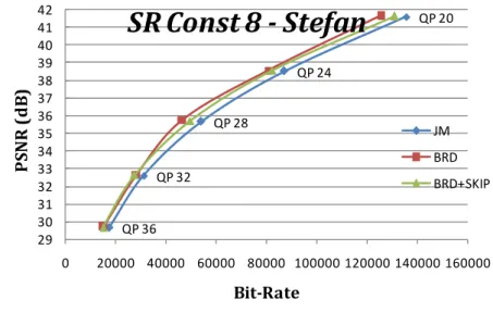
Fig. 4-11 RD curve comparison under SR constant 8 for “Stefan” sequence ... 40
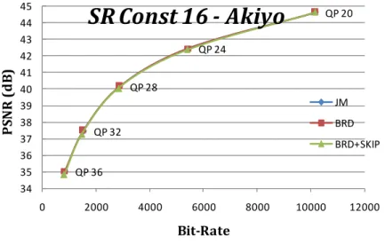
Fig. 4-12 RD curve comparison under SR constant 16 for “Akiyo” sequence ... 41
Fig. 4-13 RD curve comparison under SR constant 16 for “Foreman” sequence ... 41
Fig. 4-14 RD curve comparison under SR constant 16 for “Stefan” sequence ... 41
Fig. 4-15 RD curve comparison under SR constant 24 for “Akiyo” sequence ... 42
Fig. 4-16 RD curve comparison under SR constant 24 for “Foreman” sequence ... 42
Fig. 4-17 RD curve comparison under SR constant 24 for “Stefan” sequence ... 42
Fig. 4-18 RD curve comparison under SR random 8 for “Akiyo” sequence ... 43
Fig. 4-19 RD curve comparison under SR random 8 for “Foreman” sequence ... 43
Fig. 4-20 RD curve comparison under SR random 8 for “Akiyo” sequence ... 43
Fig. 4-21 RD curve comparison under SR random 16 for “Akiyo” sequence ... 44
Fig. 4-22 RD curve comparison under SR random 16 for “Foreman” sequence ... 44
Fig. 4-23 RD curve comparison under SR random 16 for “Stefan” sequence ... 44
Fig. 4-24 RD curve comparison under SR random 24 for “Akiyo” sequence ... 45
Fig. 4-25 RD curve comparison under SR random 24 for “Foreman” sequence ... 45
Fig. 4-26 RD curve comparison under SR random 24 for “Stefan” sequence ... 45
Fig. 4-27 The distribution of MB for “Akiyo” sequence ... 47
Fig. 4-28 The distribution of MB for “foreman” sequence ... 47
Fig. 4-29 The distribution of MB for “Stefan” sequence ... 47
Fig. 4-30 Coding time curve with skip detection of CIF sequences under: (a) SR constant 8 (b) SR constant 16 (c) SR constant 24 (d) SR random 8 (e) SR random 16 (f) SR random 24 patterns ... 49
Fig. 4-31 Completion time comparison under SR random 8 pattern ... 50
Fig. 4-32 Completion time comparison under SR random 16 pattern ... 50
Fig. 4-33 Completion time comparison under SR random 24 pattern ... 51
Fig. 4-34 Illustration of completion time comparison under different SR random pattern ... 51
Fig. 5-1 BRD optimized motion estimation algorithm hardware architecture ... 53
XI
L
L
i
i
s
s
t
t
o
o
f
f
T
T
a
a
b
b
l
l
e
e
TABLE 3-1 Boundary determination of QP 28 (mean, variance, boundary and maxima
for the 4x4-block SAD distribution which higher than T0) ... 14
TABLE 3-2 Spike threshold under different QP ... 14
TABLE 3-3 Boundary determination under different QP ... 14
TABLE 3-4 The boundary and SAD value under QP28 of different sequences ... 15
TABLE 3-5 The boundary and SAD value under QP 28 of different sequences (Normalized to Akiyo) ... 15
TABLE 4-1 Bandwidth usage of one MB ... 29
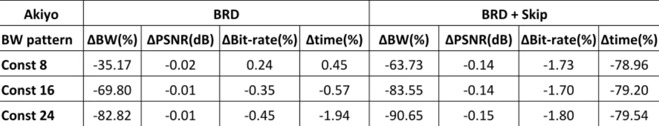
TABLE 4-2 Performance of BRD and BRD + Skip model under SR const pattern for “Akiyo” sequence ... 33
TABLE 4-3 Performance of BRD and BRD + Skip model under SR const pattern for “Foreman” sequence ... 33
TABLE 4-4 Performance of BRD and BRD + Skip model under SR const pattern for “Stefan” sequence ... 33
TABLE 4-5 Performance of BRD and BRD + Skip model under SR random pattern for “Akiyo” sequence ... 33
TABLE 4-6 Performance of BRD and BRD + Skip model under SR random pattern for “Foreman” sequence ... 33
TABLE 4-7 Performance of BRD and BRD + Skip model under SR random pattern for “Stafen” sequence ... 33
TABLE 4-8 RD comparison of BRD and BRD + Skip model under SR constant 8 for “Akiyo” sequence ... 37
TABLE 4-9 RD comparison of BRD and BRD + Skip model under SR constant 8 for “Foreman” sequence ... 37
TABLE 4-10 RD comparison of BRD and BRD + Skip model under SR constant 8 for “Stefan” sequence ... 37
TABLE 4-11 RD comparison of BRD and BRD + Skip model under SR constant 16 for “Akiyo” sequence ... 37
TABLE 4-12 RD comparison of BRD and BRD + Skip model under SR constant 16 for “Foreman” sequence ... 37
XII
TABLE 4-13 RD comparison of BRD and BRD + Skip model under SR constant 16 for “Stefan” sequence ... 37 TABLE 4-14 RD comparison of BRD and BRD + Skip model under SR constant 24 for
“Akiyo” sequence ... 38 TABLE 4-15 RD comparison of BRD and BRD + Skip model under SR constant 24 for
“Foreman” sequence ... 38 TABLE 4-16 RD comparison of BRD and BRD + Skip model under SR constant 24 for
“Stefan” sequence ... 38 TABLE 4-17 RD comparison of BRD and BRD + Skip model under SR random 8 for
“Akiyo” sequence ... 38 TABLE 4-18 RD comparison of BRD and BRD + Skip model under SR random 8 for
“Foreman” sequence ... 38 TABLE 4-19 RD comparison of BRD and BRD + Skip model under SR random 8 for
“Stefan” sequence ... 38 TABLE 4-20 RD comparison of BRD and BRD + Skip model under SR random 16 for
“Akiyo” sequence ... 39 TABLE 4-21 RD comparison of BRD and BRD + Skip model under SR random 16 for
“Foreman” sequence ... 39 TABLE 4-22 RD comparison of BRD and BRD + Skip model under SR random 16 for
“Stefan” sequence ... 39 TABLE 4-23 RD comparison of BRD and BRD + Skip model under SR random 24 for
“Akiyo” sequence ... 39 TABLE 4-24 RD comparison of BRD and BRD + Skip model under SR random 24 for
“Foreman” sequence ... 39 TABLE 4-25 RD comparison of BRD and BRD + Skip model under SR random 24 for
“Stefan” sequence ... 39 TABLE 4-26 Coding time with skip detection of CIF sequences under: (a) SR constant 8
(b) SR constant 16 (c) SR constant 24 (d) SR random 8 (e) SR random 16 (f) SR random 24 patterns ... 48
1
1
1
.
.
I
I
n
n
t
t
r
r
o
o
d
d
u
u
c
c
t
t
i
i
o
o
n
n
1
1
.
.
1
1
.
.
B
B
a
a
c
c
k
k
g
g
r
r
o
o
u
u
n
n
d
d
The emerging popular multimedia technology, such as digital television, mobile phone and DVD player bring us convenience in daily life. However, the data amount of video is too large to transmit or record without compression techniques. Therefore, several compression techniques have been proposed to reduce the data and bandwidth efficiently. The H.264/AVC standard [1] has been adopted recently as a popular compression technique from its high compression rate. In which, motion estimation (ME) part is the most computational and memory intensive component in H.264 encoder. To support these high computation and high bandwidth on ME, several algorithms have been proposed. However, traditional ME algorithms focus on rate and distortion performance, and thus do not take memory bandwidth into consideration. While coding under bandwidth constraint, it will lead to a significant quality loss or the coding time will be delayed. Therefore, the rate and distortion performance are not optimized under bandwidth constraint.
2
1
1
.
.
2
2
.
.
M
M
o
o
t
t
i
i
v
v
a
a
t
t
i
i
o
o
n
n
a
a
n
n
d
d
c
c
o
o
n
n
t
t
r
r
i
i
b
b
u
u
t
t
i
i
o
o
n
n
The issue mentioned above motivates us to develop rate distortion optimized motion estimation under the available memory bandwidth constraint. The bandwidth-rate-distortion optimized concept has a lot of similarities with the power-aware design [8][9][10][11] and computation-aware design [12][13][14][15][16], and both these designs develop as a basis of rate-control-like procedure. Therefore, we propose a rate-control-like procedure for macroblock (MB)-level bandwidth allocation, which not only meets the bandwidth constraint, but also maximizes the coding efficiency.
The contribution of the thesis is described as follows:
We proposed a bandwidth-rate-distortion (B-R-D) optimized motion estimation algorithm. The concept has three phases including
1) We propose a simple skip mode detection with content-aware scheme to find if that is a skipped MB for saving the most memory bandwidth.
2) We propose a bandwidth-rate-distortion (B-R-D) optimize modeling method to decide a feasible search range (SR) while can dynamically meet the available bandwidth and maximize the coding efficiency.
3) We propose a SR boundary prediction method to determine a feasible SR boundary for SR refinement.
1
1
.
.
3
3
.
.
T
T
h
h
e
e
s
s
i
i
s
s
o
o
r
r
g
g
a
a
n
n
i
i
z
z
a
a
t
t
i
i
o
o
n
n
In chapter 2, we give an overview of the environment-aware motion estimation algorithms. In chapter 3, we propose a B-R-D optimized ME algorithm to maximize rate distortion efficiency while can dynamically meet the available bandwidth. In chapter 4, we show the simulation result and analysis. In chapter 6, we implement the hardware of the B-R-D optimized ME algorithm. Conclusion and future work are given in chapter 7.
3
2
2
.
.
O
O
v
v
e
e
r
r
v
v
i
i
e
e
w
w
o
o
f
f
e
e
n
n
v
v
i
i
r
r
o
o
n
n
m
m
e
e
n
n
t
t
a
a
w
w
a
a
r
r
e
e
m
m
o
o
t
t
i
i
o
o
n
n
e
e
s
s
t
t
i
i
m
m
a
a
t
t
i
i
o
o
n
n
a
a
l
l
g
g
o
o
r
r
i
i
t
t
h
h
m
m
s
s
Motion estimation (ME) part is the most important component in H.264 encoder. In which, the variable block size integer-pel motion estimation (IME) not only contributes a lot for coding efficiency but also dominate the computation, power, and bandwidth loading of the whole encoding process. To support high performance under limited computation, power, and bandwidth, various environment-aware motion estimations have been proposed. The environment-aware motion estimation means that it has several modes of motion estimation process, and could dynamically adapts its operating configurations based on the awareness of environmental conditions, such as computation-constrained, power-constrained, bandwidth-constrained or user preferences.
In this chapter, we first introduce variable block-based motion estimation as a basis of the following sections. And then, we review the environment-aware motion estimation algorithms as follows:
1) Adaptive search range motion estimation 2) Power-aware motion estimation
3) Computation-aware motion estimation 4) Skip mode detection algorithm
2
2
.
.
1
1
.
.
O
O
v
v
e
e
r
r
v
v
i
i
e
e
w
w
o
o
f
f
v
v
a
a
r
r
i
i
a
a
b
b
l
l
e
e
b
b
l
l
o
o
c
c
k
k
‐
‐
b
b
a
a
s
s
e
e
d
d
m
m
o
o
t
t
i
i
o
o
n
n
e
e
s
s
t
t
i
i
m
m
a
a
t
t
i
i
o
o
n
n
The block-based motion estimation is the most widely used motion estimation method for video coding, since most of the pictures are normally rectangular in shape and block-division can be easily done. In H.264 [2], the standard adopts hierarchical variable block size motion estimation technique to improve the accuracy. Fig. 2-1(a) shows the
4
mode hierarchy and Fig. 2-1(b) shows the mode type and its block size. In one frame, it consists of several macroblocks (MB), which are “16 by 16” pixels square. In one macroblock, it can be divided into four “8 by 8” pixels 8x8 blocks. And within one 8x8 block, it can be further divided into four “4 by 4” pixels 4x4 blocks. Fig. 2-2 illustrates the shape of various block size as listed in Fig. 2-1(b). For the video with complex textures, the smaller blocks will provide better coding efficiency but with more motion vectors. In contrast, as for the video with smooth textures, the larger blocks will provide better coding efficiency with fewer motion vectors.
Fig. 2-1 (a)The mode hierarchy and (b) its block size for H.264
Fig. 2-2 Different modes for H.264 motion estimation
…
~
~
Mode Block size
Mode 1 16 x 16 Mode 2 16 x 8 Mode 3 8 x 16 Mode 4 8 x 8 Mode 5 8 x 4 Mode 6 4 x 8 Mode 7 4 x 4 16 8 4 16x16 8x16 8x16 16x8 16x8 8x8 8x8 8x8 8x8 8x8 8x4 8x4 4x8 4x8 4x4 4x4 4x4 4x4
Mode 1 Mode 2 Mode 3 Mode 4
5
2
2
.
.
2
2
.
.
R
R
e
e
v
v
i
i
e
e
w
w
o
o
f
f
a
a
d
d
a
a
p
p
t
t
i
i
v
v
e
e
s
s
e
e
a
a
r
r
c
c
h
h
r
r
a
a
n
n
g
g
e
e
m
m
o
o
t
t
i
i
o
o
n
n
e
e
s
s
t
t
i
i
m
m
a
a
t
t
i
i
o
o
n
n
Because of the motion estimation in H.264 induces a high computational complexity and leads high power consumption. Several motion estimation algorithms for low complexity and low power have been proposed. However, most of the traditional fast motion estimation algorithms reduce the complexity or power with more or less image quality sacrifice that compared with the full search motion estimation. For this reason, there is an approach to reduce the complexity or power by adjusting the search range size to suit the motion level of a video sequence. In Tian’s algorithm [4] and In Toru’s algorithm [5], an appropriate search range is determined on the basis of neighboring motion vectors (MV) (i.e. as shown in Fig. 2-3) and prediction errors due to spatial correlation between neighboring blocks and current block. And in Shih’s algorithm [6], it adjusts the horizontal and vertical search ranges independently since there have no relationship between horizontal motion and vertical motion. In addition, to serve different resolution video content, Wang’s algorithm [7] particularly adjusts the search range on the basis of the quantization parameter and the input size.In above algorithms, narrow search ranges are chosen for slow motion to reduce the complexity and power without quality degradation while wide search ranges are chosen for high motion to maintain the quality.
6
2
2
.
.
3
3
.
.
R
R
e
e
v
v
i
i
e
e
w
w
o
o
f
f
p
p
o
o
w
w
e
e
r
r
‐
‐
a
a
w
w
a
a
r
r
e
e
m
m
o
o
t
t
i
i
o
o
n
n
e
e
s
s
t
t
i
i
m
m
a
a
t
t
i
i
o
o
n
n
Power-aware design concept has been introduced recently due to supporting high computation and high bandwidth on mobile devices. A power-aware design is not only a low power design, but also aware the environment to execute the functions with limited power. Traditional ME design is considered for worst case, and therefore always uses full energy no matter whether the execution is easy or difficult. However, it leads on unnecessary power consumption and shortens the lifetime of devices. Thus to fully utilize the available power in an efficient way, several power-aware designs have been proposed. In [8], it focuses on the introduction of power-aware concepts and considerations to the architecture design of a video coder as shown in Fig. 2-4, including the discussions of power-aware motion estimation and discrete cosine transform. And in motion estimation, it adopts several fast algorithms, and several skills like bit truncation scheme and sub-sampling for multiple power modes support. In [9] and [10], they propose a dedicated hardware with reconfigurable macroblock pipelining architecture for adopting its motion estimation pre-skip algorithm. Through the pre-skip algorithm, the power can be efficiently utilized, thus the power scalability can be improved for more power management. And in [11], it develops a power-rate-distortion (P-R-D) model for optimizing the rate-distortion (R-D) behavior under the power constraints. By using the P-R-D model, given a power supply level and a bit rate, the power-scalable video is able to find the best configuration of complexity control to maximize the video quality.
7
Fig. 2-4 Power aware multimedia systems [8]
2
2
.
.
4
4
.
.
R
R
e
e
v
v
i
i
e
e
w
w
o
o
f
f
c
c
o
o
m
m
p
p
u
u
t
t
a
a
t
t
i
i
o
o
n
n
‐
‐
a
a
w
w
a
a
r
r
e
e
m
m
o
o
t
t
i
i
o
o
n
n
e
e
s
s
t
t
i
i
m
m
a
a
t
t
i
i
o
o
n
n
Many fast algorithms reduce the computation complexity of motion estimation to meet the computation constraints, and thus lead to significant quality loss. Therefore, several computation-aware ME algorithms have been proposed while can dynamically adjust the target function under limited computation resource. In [12], its proposed computation-aware scheme can dynamically determine the target computation which is allocated to each frame, and then to each block in a computation-distortion-optimized manner. The mean-square-error difference obtained from initial motion vector and best motion vector is regarded as a distortion gain measure under computation constraints, and thus can achieve better coding efficiency by adopting its computation-aware scheme. In [13], it develops a complexity-rate-distortion framework, which extends the traditional R-D analysis by including another dimension, the computation complexity. This framework determines for each MB which partitions are likely to be optimal and motion vector search is only carried out for only the selected partitions, thus reducing the complexity of the ME step. In [14], Through investigating various issues in H.264, such as
8
complexity prediction methods, MB complexity scaling and time scheduling algorithms, it proposes a method based on dynamic control of the encoding parameters to meet real-time constraints while minimizing coding efficiency loss. In [15], it uses the sum of absolute components of predict motion vectors to help allocating the available computation to a frame, and then the computation to a frame is distributed to MBs. And in [16], it presents a complexity aware motion estimation for H.624 based on pixel representation of different bit-depth and a simple scene change detection module.
2
2
.
.
5
5
.
.
R
R
e
e
v
v
i
i
e
e
w
w
o
o
f
f
s
s
k
k
i
i
p
p
m
m
o
o
d
d
e
e
d
d
e
e
t
t
e
e
c
c
t
t
i
i
o
o
n
n
a
a
l
l
g
g
o
o
r
r
i
i
t
t
h
h
m
m
In MPEG-4 AVC/H.264 video coding, integer-pel motion estimation (IME) and fraction-pel motion estimation (FME) contribute a lot for coding efficiency due to new techniques, such as variable block size and six-tap interpolation filter. However, these new complex techniques make ME dominate the computational loading and power of the whole encoding process up to 96% [15]. The most efficient way to lower the complexity and power of ME is to directly skip the MB encoding and simply denotes it with skip mode if the encoding situation is allowed. Therefore, as long as we can predict the skip mode before ME, we can skip the whole coding stage and save encoding power of this skipped MB. And in H.264/AVC, the MB will be skipped without encoding the motion vectors and residues and is denoted as skip mode if the following conditions are matched:
1) The chosen block type is 16x16 (Mode 1).
2) The best motion vector equals the predicted motion vector (MVP). 3) The chosen frame is the previous frame.
9
2
2
.
.
5
5
.
.
1
1
.
.
L
L
a
a
g
g
r
r
a
a
n
n
g
g
i
i
a
a
n
n
c
c
o
o
s
s
t
t
m
m
o
o
t
t
i
i
o
o
n
n
e
e
s
s
t
t
i
i
m
m
a
a
t
t
i
i
o
o
n
n
In [18], [19] and [20], they propose a skip prediction through Lagrangian cost function. The paper [18] uses a Lagrangian rate-distortion cost function which incorporates an adaptive model for the Lagrangian multiplier parameter base on local sequence statistics. The paper [19] predicts the Lagrangian multiplier parameter from the statistical dependency of previous co-located block. And the paper [20], the skip decision is based on a partially computed SAD metric combined with utilization of the Lagrangian cost function from the previous frame.
2
2
.
.
5
5
.
.
2
2
.
.
A
A
l
l
l
l
z
z
e
e
r
r
o
o
D
D
C
C
T
T
b
b
l
l
o
o
c
c
k
k
s
s
d
d
e
e
t
t
e
e
c
c
t
t
i
i
o
o
n
n
In [21], [22] and [23], they perform a comprehensive analysis of the dynamic properties of the DCT and quantization in H.264. They use several partial sum of absolute differences (SADs) in a 4x4 block to predict the zero blocks in various conditions. And in [24], a classifier based on the absolute frame differences has been employed to detect the zero blocks to effectively skip unnecessary modes and reference frames.
10
11
3
3
.
.
P
P
r
r
o
o
p
p
o
o
s
s
e
e
d
d
B
B
R
R
D
D
o
o
p
p
t
t
i
i
m
m
i
i
z
z
e
e
d
d
m
m
o
o
t
t
i
i
o
o
n
n
e
e
s
s
t
t
i
i
m
m
a
a
t
t
i
i
o
o
n
n
a
a
l
l
g
g
o
o
r
r
i
i
t
t
h
h
m
m
Motion estimation (ME) part is the most computational and memory intensive component in H.264 encoder. Traditional ME design focuses on its rate distortion performance, and thus assumes a worst case memory bandwidth requirement to the whole system. However, such assumption ignores the realistic facts of diverging contents and varying available memory bandwidth in a whole system. Diverging contents imply worst case requirement to be an overdesign or waste. Varying bandwidth could limit the available data and thus degrade the video quality or fail the real time constraints. Thus, in this thesis, we propose a rate-distortion optimized motion estimation design while can dynamically meet the available bandwidth, which is called bandwidth-rate-distortion (B-R-D) optimized motion estimation.
The rest of chapter is organized as follows. We will first introduce the whole B-R-D optimized ME algorithms. Then we will discuss each part in details in the rest of the chapter.
12
3
3
.
.
1
1
.
.
I
I
n
n
t
t
r
r
o
o
d
d
u
u
c
c
t
t
i
i
o
o
n
n
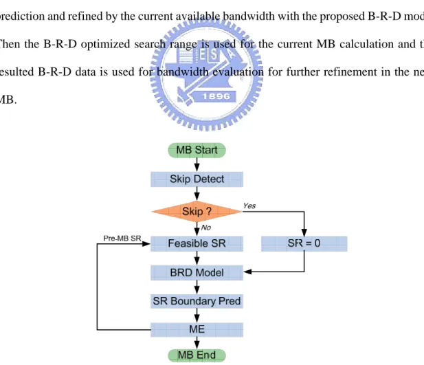
The overall B-R-D optimized ME is shown in Fig. 3-1. This algorithm is developed with the following concepts. First, the target problem is to develop rate distortion optimized motion estimation under the available memory bandwidth constraint. To make the maximum use of the bandwidth, we first adopt a simple skip mode detection to find if that is a skipped MB. A skipped MB implies the lowest memory bandwidth ME (zero search range) and thus gives other complex MB more bandwidth for better quality. Thus, for other non-skipped MBs, they go through two steps for optimization: bandwidth prediction and bandwidth evaluation. Note that bandwidth is determined by the search range. Thus, bandwidth prediction is first determined by initial search range boundary prediction and refined by the current available bandwidth with the proposed B-R-D model. Then the B-R-D optimized search range is used for the current MB calculation and the resulted B-R-D data is used for bandwidth evaluation for further refinement in the next MB.
13
3
3
.
.
2
2
.
.
P
P
r
r
o
o
p
p
o
o
s
s
e
e
d
d
s
s
k
k
i
i
p
p
m
m
o
o
d
d
e
e
d
d
e
e
t
t
e
e
c
c
t
t
i
i
o
o
n
n
w
w
i
i
t
t
h
h
c
c
o
o
n
n
t
t
e
e
n
n
t
t
‐
‐
a
a
w
w
a
a
r
r
e
e
s
s
c
c
h
h
e
e
m
m
e
e
This algorithm is based on our previous work [23] with some refinement. The object of the algorithm is to detect a zero MB with content-aware scheme, and save the most memory bandwidth for other complex MB coding. The whole algorithm is illustrated in Fig. 3-2. First, we detect whether a 4x4-block is zero or not by a refined SAD-4x4-block threshold, and count the number of zero-4x4-blocks in a MB. If the number is larger than MB-zero-block threshold, we refer to this current MB as a zero MB and skip this coding. In addition, to avoid above SAD threshold affected by local large variations, we adopt a spike threshold to remove such cases for more accurate detection. More details are described in the following.
Fig. 3-2 Skip mode detection flow
3
3
.
.
2
2
.
.
1
1
.
.
R
R
e
e
v
v
i
i
e
e
w
w
o
o
f
f
S
S
A
A
D
D
‐
‐
4
4
x
x
4
4
‐
‐
b
b
l
l
o
o
c
c
k
k
t
t
h
h
r
r
e
e
s
s
h
h
o
o
l
l
d
d
From our previous work [23], the SAD-4x4-block threshold is used to decide if a 4x4-block is zero. We determine the threshold by analyzing the distribution of the
Count zero-4x4-blocks
No. of zero-4x4-blocks > MB-zero-block threshold ?
Get zero-4x4-block threshold
(With refinement)
Get MB-zero-block threshold
No any 4x4-block sad > spike threshold ? N N Y Y Start Pre-Skip Not Pre-Skip
14
4x4-block SADs higher than the must-be-zero-block threshold [22](Denote it by T0), but also quantized to zero block in skipped MB. We analyze five 300-frame CIF size test sequences to determine this threshold as shown in TABLE 3-1. In which, the “mean”, variance, “maxima” stand for the average, standard variation and maxima values of 4x4-blocks whose SADs are higher than T0. The boundary that we refer to as the SAD-4x4-block threshold is the summation of mean and variance.
From TABLE 3-1, we can find that almost 85.9% in average of the 4x4-block SADs in one skip MB is less than the boundary. When the SAD of the 4x4-block is less than the boundary, we refer to the 4x4-block as a zero block. Therefore, we choose the SAD-4x4-block threshold to prevent from large prediction error. And the SAD-4x4-block threshold under different QPs is shown in TABLE 3-3.
TABLE 3-1 Boundary determination of QP 28 (mean, variance, boundary and maxima for the 4x4-block SAD distribution which higher than T0)
QP 28 Mean Variance Boundary Maxima
Akiyo 44.3 10.6 55 111
Mother 45.1 9.9 55 97
Foreman 45.4 10.3 56 103
Football 50.8 11.4 62 103
Silence 55.9 12.8 69 109
TABLE 3-2 Spike threshold under different QP
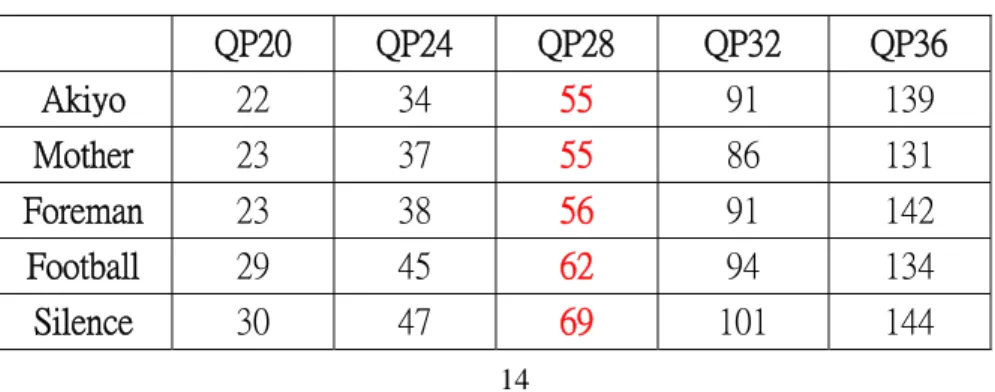
TABLE 3-3 Boundary determination under different QP
QP20 QP24 QP28 QP32 QP36 Akiyo 22 34 55 91 139 Mother 23 37 55 86 131 Foreman 23 38 56 91 142 Football 29 45 62 94 134 Silence 30 47 69 101 144 QP20 QP24 QP28 QP32 QP36 Spike threshold 37 66 97 160 230
15
3
3
.
.
2
2
.
.
2
2
.
.
R
R
e
e
f
f
i
i
n
n
e
e
m
m
e
e
n
n
t
t
o
o
f
f
S
S
A
A
D
D
‐
‐
4
4
x
x
4
4
‐
‐
b
b
l
l
o
o
c
c
k
k
t
t
h
h
r
r
e
e
s
s
h
h
o
o
l
l
d
d
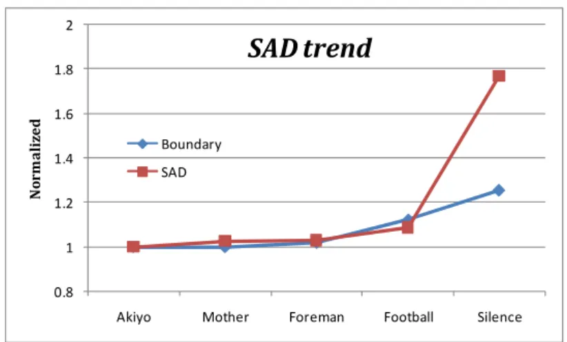
In this section, we analyze the relationship between prediction error and SAD-4x4-block threshold to help with refining the SAD-4x4-block threshold that presented from section 3.2.1. From TABLE 3-4 and TABLE 3-5, we found that both SAD-4x4-block threshold and SAD have high correlation as shown in Fig. 3-3. According to above relationship, we make a list including SAD and boundary information as shown in Fig. 3-4(a), and use this list to dynamically adjust SAD-4x4-block threshold from the prediction error under different QP as shown in Fig. 3-4(b)-(f). We can see that the SAD-4x4-block threshold is much proportion to SAD in lower QP cases. Thus such cases will make a better approximation with SAD-4x4-block threshold refinement.
TABLE 3-4 The boundary and SAD value under QP28 of different sequences
Original Akiyo Mother Foreman Football Silence
Boundary 55 55 56 62 69
SAD 757 776 779 822 1337
TABLE 3-5 The boundary and SAD value under QP 28 of different sequences (Normalized to Akiyo)
Normalized Akiyo Mother Foreman Football Silence
Boundary 1 1 1.018 1.127 1.254
SAD 1 1.025 1.029 1.086 1.768
Fig. 3-3 The trend between boundary and SAD (Normalized to Akiyo) 0.8 1 1.2 1.4 1.6 1.8 2
Akiyo Mother Foreman Football Silence
No rm al iz ed
SAD trend
Boundary SAD16
Fig. 3-4 (a) SAD and SAD-4x4-block threshold under different QP
Threshold estimation under (b) QP20 (c) QP24 (d) QP28 (e) QP32 (f) QP36
3
3
.
.
3
3
.
.
P
P
r
r
o
o
p
p
o
o
s
s
e
e
d
d
B
B
‐
‐
R
R
‐
‐
D
D
o
o
p
p
t
t
i
i
m
m
i
i
z
z
e
e
d
d
m
m
o
o
d
d
e
e
l
l
i
i
n
n
g
g
m
m
e
e
t
t
h
h
o
o
d
d
In this section, a bandwidth-rate-distortion (B-R-D) optimized modeling method is proposed as shown in Fig. 3-5. The method is developed with the following concepts. First, to make maximum use of the bandwidth from bus system, we transform this bandwidth into an available system search range for bandwidth budget estimation. According to the bandwidth budget, we make an appropriate bandwidth allocation for further MB coding process. Then, to justify the coding efficiency under a given bandwidth, we define a bandwidth efficiency Gave up to i-th MB. And we adopt Gave,
rate-distortion cost, and usable bandwidth budget to make a bandwidth prediction for
20 22 24 26 28 30 32 700 800 900 1000 1100 1200 1300 1400 Th re sh ol d SAD Threshold estimation QP 20 4x4‐block‐ threshold 32 34 36 38 40 42 44 46 48 700 800 900 1000 1100 1200 1300 1400 Th re sh ol d SAD Threshold estimation QP 24 4x4‐block‐ threshold 54 56 58 60 62 64 66 68 70 700 800 900 1000 1100 1200 1300 1400 Th re sh ol d SAD Threshold estimation QP 28 4x4‐block‐ threshold 80 83 86 89 92 95 98 101 700 800 900 1000 1100 1200 1300 1400 Th re sh ol d SAD Threshold estimation QP32 4x4‐block‐ threshold 126 130 134 138 142 146 150 700 800 900 1000 1100 1200 1300 1400 Th re sh ol d SAD Threshold estimation QP36 4x4‐block‐ threshold (a) (b) (c) (d) (e) (f)
Akiyo Mother Foreman Football Silence SAD 757 776 779 822 1337 QP20 thre 22 23 23 29 30 QP24 thre 34 37 38 45 47 QP28 thre 55 55 56 62 69 QP32 thre 91 86 91 94 101 QP36 thre 139 131 142 134 144
17 1 GOP Frame
Default SR
BW budget !
keeping quality smoothness. Afterward, to make maximum use of the bandwidth budget, we make a bandwidth boundary prediction by considering the bandwidth prediction condition to determine a feasible bandwidth interval. Finally, we employ this interval and certain rate distortion data to make a search range decision and set an appropriate search range for further ME use. More details are as follows:
Fig. 3-5 B-R-D optimized modeling method flow
Step 1: Bandwidth (BW) budget initialization
First, according to bus status and user’s preferences, we calculate the system search range for bandwidth budget estimation. Then, we initialize the bandwidth budget for bandwidth allocation in later coding process as shown in Fig. 3-6. Both system search range and bandwidth budget equation are defined as follows:
Default_ SR = ⎥ ⎥ ⎥ ⎥ ⎦ ⎥ ⎢ ⎢ ⎢ ⎢ ⎣ ⎢ − 2 16 _ _ _ *
_rate MBs in one frame Frame
BWBus
BWbudget = ( 2*Default_SR + 16 ) * ( 2*Default_SR + 16 )*
18
In which, the word BWBus denotes the bus data transmission rate (MBps), Frame_rate
denotes coded frame numbers per second, MBs_in_one_frame denotes MB numbers per frame, Default_SR denotes default search range in a group of picture (GOP), and
GOP_size denotes frame numbers in a GOP. While coding at the beginning of GOP, our
design receive data transmission rate supplied from the bus system. To make maximum use of the bandwidth from bus system, we transform this rate into a default search range, and use this default search range to estimate a bandwidth budget. Base on this bandwidth budget, we allocate appropriate bandwidth within a GOP for better quality maintain. For ease of decision, we set the bandwidth budget for a GOP with 16 frames.
Step 2: B-R-D performance calculation
To justify the bandwidth usage, we define the bandwidth efficiency Gave up to i-th MB
as follows. ∑− = ∑− = − = 1 1 1 1 i ) ( k i i usage BW k i BMA RDC i init RDC ave G
In which, letRDCiniti denotes the rate-distortion cost that obtained using the initial MV
(i.e. MVP),
RDC
BMAi denotes the rate-distortion cost that obtained after a motion searchfrom block-matching algorithm (BMA) (i.e. Full search algorithm), andBWusagei denotes
actual BW usage that performed in previous k-1 MB. Gave means the average
rate-distortion gain of a given bandwidth. The more Gave we gain, the better coding
efficiency we will perform. In the following step, we will use Gave for bandwidth
19
Step 3: Bandwidth prediction
In this step, the objective of bandwidth prediction is to predict usable bandwidth for next MB. First, to keep the quality smoothness between the current and the previous MBs, we adopt certain data from previous MBs for further prediction as shown in Fig. 3-7. The following equation should hold:
1 1 1 BMA G - − ∑− = = k k i i RDC k BP BW ave k init RDC
Let BWBPk be the backward bandwidth prediction. Where the left-hand side of the
equation stands for the target rate distortion cost (RDC) of the current MB, the right-hand side of the equation is the averaged RDC value of the previous MB. While we obtained larger Gave from the former step, it means the less bandwidth (i.e.BWBPk ) we need for
maintaining the rate distortion gain (RDG) of the previous MB. Therefore, the backward prediction for the current MB k can be derived as
ave G k k i i RDC k init RDC k BP BW 1 1 1 BMA − − = − = ∑
In contrast toBWBPk , we define the forward predictionBW FPk for further prediction to
keep the quality smoothness between the current and the future MB by adopting certain bandwidth information as shown in Fig. 3-7. The equation is as follows:
) 1 ( 1 1 − − ∑− = − = k n k i i usage BW budget BW k FP BW
Because we have no knowledge of the future RDG performance, and therefore the forward predictionBWFPk is equal to the remaining bandwidth budget divided by the
20
Fig. 3-7 Illustration of BW prediction
Step 4: Bandwidth boundary prediction
In this step, to make maximum use of the bandwidth budget, we make a bandwidth boundary prediction by considering the bandwidth prediction condition as mentioned previously to determine a feasible bandwidth interval as follows:
if (BWFP > BWBP) (condition 1) { BWlower = BWBP + 0.5 * (BWFP – BWBP) ; BWupper = BWFP + 0.25*(BWFP – BWBP) ; } else (condition 2) { BWlower = BWFP – 0.5 * (BWBP – BWFP) ; BWupper = BWFP ; }
Fig. 3-8 Illustration of bandwidth boundary determination
In which, BWlower and BWupper denotes lower and upper bound of bandwidth usage per
MB, respectively. We allow the bandwidth vary within an interval that bounded by
Cur
Pre Next
BW
BPBW
FP21
BWlower and BWupper. To consider the condition 1 as depicted above in Fig. 3-8, BWBP
smaller than BWFP implies that insufficient BW had been allocated to the previous MBs,
and thus more bandwidth could be allocated to the next MB. As a result, we set BWlower
equal to BWBP + 0.5 * (BWFP – BWBP), and set BWupper equal to BWFP + 0.25*(BWFP –
BWBP). To improve the coding efficiency under feasible bandwidth supply, above
equations imply a reasonable allocation. In contrast, to consider the condition 2 as depicted above in Fig. 3-8, BWFP smaller than or equal to BWBP implies that too much
bandwidth had been allocated to the previous MBs, and hence less bandwidth could be allocated to the next MB. In other words, to keep the smooth constraint under feasible BW supply, we should save bandwidth for further use. Note that although adopt BWBP in
bandwidth allocation for the further coding process will guarantee the average B-R-D performance as for the previous MBs, the BW allocated to the next MB is excessive that compared with BWFP. As a result, we set BWlower equal to BWFP – 0.5 * (BWBP – BWFP),
and set BWupper equal to BWFP.
Step 5: SR decision
Finally, we employ this interval and certain rate distortion data to make a search range decision and set an appropriate search range for further ME use. In the final step, we make a search range decision by considering bandwidth boundary interval and some rate distortion data. The search decision mainly divides into two phases as follows:
1) Decision for bandwidth concern 2) Decision for quality concern
22
Fig. 3-9 Illustration of SR decision
The whole decision is illustrated in Fig. 3-9. In phase 1, making a search range decision under feasible BW supply is considered. If average bandwidth usage for previous MBs is more than BWupper, the search range should be decreased for next MB. While if average
bandwidth usage for previous MBs is less than BWlower, the search should be increased for
the next MB.
Phase 2 is on the other hand. If the average bandwidth usage for previous MBs is in the interval that bounded by BWlower and BWupper, then making a search decision under
quality maintain is next to consider. If the RDG (i.e. RDCinit - RDCBMA ) in current MB is
less than the average RDG subtracted with an adaptive offset (i.e. RDCBMA/20000 ) in the
previous MBs, the search range should be decreased for next MB. Because in spite of the coding is under feasible bandwidth supply, the rate distortion performance could not be maintained with previous MBs. In contrast, if the RDG in current MB is more than the average RDG added with an adaptive offset in previous MBs, the search range should be increased for next MB. Otherwise, if the RDG in current MB is in the interval that bounded by RDGave + offset and RDGave + offset, the search range should be hold.
Meanwhile, a special case must be considered. To avoid the terrible quality loss, the search range no longer be decreased as mentioned above. Instead, the search range could be increased by checking rate multiplied distortion (R×D). If R×D in current MB is more than average 4×R×D, the search range should be increased. After the search has decided,
RDGave+ offset BWupper BWlower SR_down SR_up BW budget RDC pool RDGave- offset
SR_down Constant SR_up
RxD pool RxDave+ offset
SR_up
BW concern
23
the search window will be updated that corresponds to the new search range as shown in Fig. 3-10.
Fig. 3-10 Illustration of SR modification
The total search range decision is shown as follows:
if (BWave > BWupper)
{
SR_down= 8 ; }
else if (BWave < BWlower)
{ SR_up = 8 ; } else { if (RxDcur > RxDave x4) { SR_up = 16 ; } else {
if (RDC_gaincur < RDC_gainave - offset)
{
SR_up = 4 ; }
else if (RDC_gaincur > RDC_gainave + offset)
{
SR_down = 4 ; }
} }
24
3
3
.
.
4
4
.
.
S
S
R
R
b
b
o
o
u
u
n
n
d
d
a
a
r
r
y
y
p
p
r
r
e
e
d
d
i
i
c
c
t
t
i
i
o
o
n
n
m
m
e
e
t
t
h
h
o
o
d
d
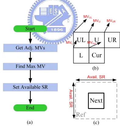
The objective of search range boundary prediction method is presented to refine the SR that had decided from section 3.3 by determining a feasible search range boundary and it could avoid unnecessary bandwidth waste for further ME use. The search range boundary prediction method is illustrated in Fig. 3-11(a). First, we get the adjacent motion vectors (MV) from neighboring blocks and current block (co-located block of previous frame), such as MVUL, MVU, MVUR, MVL, MVCur. These blocks are local maximum MV
within their own blocks, and the relationship between neighboring blocks and current block are shown as Fig. 3-11(b). Second, we compare with these five local maximum MV that mentioned above, and choose a global maximum MV. Finally, we set the available search range by referring to global maximum MV for next block coding as shown in Fig. 3-11(c).
Fig. 3-11(a) Search range boundary predicted method flow
(b) The relationship between neighboring blocks and current block (c) Example of available SR for next block coding
25
The search range boundary corresponding to MVs is shown as follows:
if (max_mv<=2) max_avail_SR = 4; else if(max_mv<=4) max_avail_SR = 8; else if(max_mv<=8) max_avail_SR = 12; else if(max_mv<=12) max_avail_SR = 16; else if(max_mv<=16) max_avail_SR = 20; else if(max_mv<=20) max_avail_SR = 24; else if(max_mv<=24) max_avail_SR = 28; else max_avail_SR = 32;
3
3
.
.
5
5
.
.
S
S
u
u
m
m
m
m
a
a
r
r
y
y
In this chapter, we propose a B-R-D optimized ME algorithm in H.264 video coding. To summarize, we first detect a MB whether it skip or not by skip mode detection with content-aware scheme. Then according to the current SR, BW status and data characteristics, we make a SR decision for next MB coding from B-R-D optimized modeling method. Finally, the SR decided before will be refined by SR boundary prediction method for further ME use. In addition, the simulation result is described in chapter 4.
27
4
4
.
.
S
S
i
i
m
m
u
u
l
l
a
a
t
t
i
i
o
o
n
n
a
a
n
n
d
d
A
A
n
n
a
a
l
l
y
y
s
s
i
i
s
s
In this chapter, we simulate the algorithms that proposed in chapter 3. First, we will introduce the bandwidth (BW) pattern which is used to stand for various bus systems. Second, we will show the experimental results as four phases:
1) Performance comparison
2) The distribution of MB for skip mode analysis 3) Timing comparison with skip detection
4) Completion time comparison of SR random patterns
Compared with the reference software [3], we can not only achieve better efficiency than JM 12.2, but also allow the motion estimation (ME) algorithm to be realized by external bus system. This is attributed to that our algorithm could save unnecessary bandwidth (BW) by detecting bus status, and then utilizing remaining BW to search more in the search window for finding better solution.
4
4
.
.
1
1
.
.
B
B
W
W
p
p
a
a
t
t
t
t
e
e
r
r
n
n
s
s
e
e
t
t
t
t
i
i
n
n
g
g
In this section, we introduce six different BW patterns to stand for various bus systems as shown in Fig. 4-1(a)-(f). These BW patterns are as follows, SR constant 8, SR constant 16, SR constant 24, SR random 8, SR random 16 and SR random 24. The numbers ‘8’, ‘16’ and ‘24’ mentioned above stand for average SR usage which are 8, 16 and 24 respectively. The word ‘constant’ represents BW supply in bus system is constant; In contrast, the word ‘random’ represents BW supply in bus system is random. The SR 8, 16 and 24 patterns are used to fit the low, medium, and high BW design respectively. Then, the SR constant pattern is used to fit the BW design with stable bus status; In contrast, the SR random pattern is used to fit the BW design with unstable bus status.