車用行動通訊網路之連線時間分析

國

立

交

通

大

學

資訊科學與工程研究所

碩 士 論 文

車用行動通訊網路之連線時間分析

Communication Time Analysis in Vehicular Ad-Hoc Networks

研 究 生：陳信帆

指導教授：陳 健 教授

車用行動通訊網路之連線時間分析

Communication Time Analysis in Vehicular Ad-Hoc Networks

研 究 生：陳信帆

Student：Hsin-Fan Chen

指導教授：陳 健

Advisor：Chien Chen

國 立 交 通 大 學

資 訊 科 學 與 工 程 研 究 所

碩 士 論 文

A Thesis

Submitted to Institute of Computer Science and Engineering College of Computer Science

National Chiao Tung University In partial Fulfillment of the Requirements

For the Degree of Master

In

Computer Science July 2007

Hsinchu, Taiwan, Republic of China

車用行動通訊網路之連線時間分析

研究生 : 陳信帆 指導教授: 陳 健 國 立 交 通 大 學 資 訊 科 學 與 工 程 研 究 所

中文摘要

近年來隨著無線網路快速發展，人們可以無所不在地使用網路，車用行動通 訊網路是無線移動網路中一種快速發展的新型態，它是由汽車的移動所構成的網 路模式，近來有不少針對車用行動通訊網路效能分析的研究，其中，大部分的研 究都是在探討通訊協定、傳送效率或是傳輸延遲，他們大部分的結果都是利用網 路模擬或是統計資料來取得。在車用行動通訊網路中，連線時間會影響到資料傳 輸與繞徑演算法的表現，所以有必要建立更精確的數學模型來正確預估其連線生 命週期，進而改善效能。所以在這篇論文中，我們提出一個數學分析模型來計算 出車用行動通訊網路在都會區中的期望連線時間，另外，我們考慮在每個十字路 口加上紅綠燈後，所造成連線時間的變化，我們一樣提出數學分析模型來分析其 期望連線時間。最後，我們將提出模擬結果來驗證期望連線時間數學模型的正確 性。 關鍵字：車用行動通訊網路、無線移動網路、連線時間

Communication Time Analysis in Vehicular

Ad-Hoc Networks

Student: Hsin-Fan Chen Advisor: Dr. Chien Chen

Institute of Computer Science and Engineering National Chiao Tung University

Abstract

Since the recent rapid development of wireless mobile networks, people can access the network ubiquitously. Vehicular ad-hoc networks (VANETs) are an emerging new type of wireless mobile ad-hoc networks (MANETs). It’s a mobile network composed of moving vehicles. There are many researches in performance for VANETs. Among those, most researches focus on the communication protocol, delivery ratio, or transmission delay. They are mostly obtained by network simulation or statistical data. In VANETs, communication time will affect data transportation and the performance of the routing algorithm. It’s necessary to build a more accurate mathematical model to estimate the communication time. In this thesis, we present a mathematical analysis model to calculate the expected communication time (ECT) of VANETs in urban city. Furthermore, we consider adding a traffic light to each intersection to observe the influence to the ECT. Finally, we present simulation results to validate our mathematical model in ECT.

誌謝

本篇論文的完成，我要感謝這兩年來給予我協助與勉勵的人。首先要感謝我 的指導教授 陳健博士，即使這段期間遭遇了不少的挫折，陳老師對我的指導與 教誨使我都能在遇到困難時另尋突破，在研究上處處碰壁時指引明路讓我得以順 利完成本篇論文，在此表達最誠摯的感謝。同時也感謝我的論文口試委員，交通 大學的曾煜棋教授、簡榮宏教授以及工業研究院的蔣村杰博士，他們提出了許多 的寶貴意見，讓我受益良多。 感謝與我一同努力的學長張哲維、陳盈羽，由於我們不斷互相討論及在論文 上的協助，使我能突破瓶頸，研究也更為完善。另外我也要感謝實驗室的同學、 學弟們，王振仰、林政一、楊智強以及楊祐華等人，感謝他們陪我度過這兩年辛 苦的研究生活，在我需要協助時總是不吝伸出援手，陪我度過最煩躁與不順遂的 日子。 最後，我要感謝家人對我的關懷及支持，他們含辛茹苦的栽培，使我得以無 後顧之憂的專心於研究所課業與研究，我要向他們致上最高的感謝。

Table of Content

中文摘要... i

Abstract ... ii

Chapter 1: Introduction ... 1

Chapter 2: Related work ... 7

Chapter 3: Expected communication time in VANETs ... 9

3.1 Opposite to Vertical Case ... 10

3.2 Parallel to Vertical case ... 17

3.3 Vertical to Opposite or Parallel case ... 23

Chapter 4: Expected Communication Time with Traffic Light ... 36

4.1 Opposite to Vertical Case with Traffic Light ... 37

4.2 Parallel to Vertical Case with Traffic Light ... 39

4.3 Vertical to Opposite or Parallel Case with Traffic Light ... 40

Chapter 5: ECT Formulation Result ... 41

5.1 ECT Formulation Result of Opposite to Vertical Case ... 41

5.2 ECT Formulation Result of Parallel to Vertical Case ... 43

5.3 ECT Formulation Result of Vertical to Opposite or Parallel Case ... 46

5.4 ECT Formulation result ... 48

Chapter 6: Formulation and Simulation Comparison ... 50

6.1 Formulation and Simulation Comparison in Opposite to vertical case ... 50

6.2 Formulation and Simulation Comparison in Parallel to vertical case ... 52

6.3 Formulation and Simulation Comparison in Vertical to Opposite or Parallel case ... 54

6.4 Formulation and Simulation Comparison of VANETs in urban city ... 55

6.5 Formulation and Simulation Comparison in Opposite to Vertical Case with Traffic Light ... 57

6.6 Formulation and Simulation Comparison in Parallel to Vertical Case with Traffic Light ... 59

6.7 Formulation and Simulation Comparison in Vertical to Opposite or Parallel Case with Traffic Light ... 61

6.8 ECT Formulation and Simulation Comparison with Traffic Light ... 63

Chapter 7: Conclusion ... 65

List of Figure

Figure 1: Random Waypoint Mobility Model ... 3

Figure 2: Manhattan Grid Mobility Model ... 3

Figure 3: Communication time ... 5

Figure 4: Number of turn during communication time ... 5

Figure 5: Opposite to Vertical Case; Parallel to Vertical Case; Vertical to Opposite or Parallel case ... 6

Figure 6: Opposite case of VANETs in urban city ... 11

Figure 7: Opposite to Vertical Case with turn probability pturn ... 12

Figure 8: Relation of s and location of MN ... 12 _A Figure 9: Parallel to vertical with turn probability pturn... 18

Figure 10: Parallel case of VANETs in urban city ... 19

Figure 11: Relation of s and location of MN ... 19 A Figure 12: Vertical case ... 23

Figure 13: Relationship between entrance point of MN and B  ... 26

Figure 14: relationship between  and r ... 26

Figure 15: Vertical case of VANETs in urban city ... 27

Figure 16: Vertical to Opposite or Parallel Case with turn probability pturn ... 28

Figure 17: Specific value of angle  ... 29

Figure 18: Value of i H  ... 30

Figure 19: Relationship between v and range of angle _B  ... 31

Figure 20: Segment of v ... 32 _B Figure 21: State of MN and A MN ... 37 B Figure 22: Opposite to Vertical Case with different turn probability ... 42

Figure 23: Opposite to Vertical Case with different gird size ... 43

Figure 24: Parallel to Vertical Case with different turn probability ... 44

Figure 25: Divide into two case v_B v_A and v_Av_B ... 45

Figure 26: Parallel to Vertical Case with different grid size ... 46

Figure 27: Vertical to Opposite or Parallel Case with different turn probability 47 Figure 28: Vertical to Opposite or Parallel Case with different grid size ... 48

Figure 29: ECT of VANETs in urban city with different turn probability ... 49

Figure 30: ECT of VANETs in urban city with different grid size ... 49

Figure 31: Formulation and Simulation Comparison in Opposite to Vertical Case ... 51

Figure 32: Formulation and Simulation Comparison in Parallel to Vertical Case ... 53

Figure 33: Formulation and Simulation Comparison in Vertical to Opposite or Parallel Case ... 54 Figure 34: Formulation and Simulation Comparison of VANETs in urban city . 56 Figure 35: Formulation and Simulation Comparison in Opposite to Vertical Case with Traffic Light ... 58 Figure 36: Formulation and Simulation Comparison in Parallel to Vertical Case with Traffic Light ... 60 Figure 37: Formulation and Simulation Comparison in Vertical to Opposite or Parallel Case with Traffic Light ... 62 Figure 38: Formulation and Simulation Comparison of VANETs in urban city with Traffic Light ... 63

List of Equation

Equation 1: ECT of VANETs in urban city ... 10

Equation 2: Calculate parameters of Opposite to Vertical Case ... 13

Equation 3: Minimum speed that v can reach number j cross ... 13 _B Equation 4: Calculate T , 1 T and 2 T of Opposite to Vertical Case ... 15 3 Equation 5: PDF of v and _B s ... 15

Equation 6: ECT formulation of Opposite to Vertical Case ... 17

Equation 7: Calculate parameters of Parallel to Vertical Case ... 20

Equation 8: Calculate T , 1 T and 2 T of Parallel to Vertical Case ... 21 3 Equation 9: ECT formulation of Parallel to Vertical Case ... 22

Equation 10: ECT formulation of Vertical Case ... 24

Equation 11: ECT of Vertical Case ... 25

Equation 12: PDF of v and _B  ... 25

Equation 13: PDF of  ... 27

Equation 14: Specific value of angle  ... 29

Equation 15: Segment of v ... 31 _B Equation 16: Calculate T , 1 T , 2 T and 3 T ... 34 4 Equation 17: ECT formulation of Vertical to Opposite or Parallel Case ... 35

Equation 18: Probability of MN and A MN stop per second ... 38 B Equation 19: Probability of each state happened ... 38

Equation 20: Multiple of communication time in Opposite to Vertical Case ... 38

Equation 21: Calculate ECT ... 39 TL Equation 22: Multiple of communication time in Parallel to Vertical Case ... 40

Equation 23: Multiple of communication time in Vertical to Opposite or Parallel Case ... 40

List of Table

Table 1: Simulation parameters of Opposite to Vertical Case ... 52

Table 2: Simulation parameters of Parallel to Vertical Case ... 53

Table 3: Simulation parameters of Vertical to Opposite or Parallel Case ... 55

Table 4: Simulation parameters of VANETs in urban city ... 56

Table 5: Simulation parameters of Opposite to Vertical Case with traffic light .. 59

Table 6: Simulation parameters of Parallel to Vertical Case with traffic light .... 61

Table 7: Simulation parameters of Vertical to Opposite or Parallel Case with traffic light ... 62

Chapter 1: Introduction

In this thesis, we mainly discuss the communication time analysis in Vehicular Ad Hoc Networks (VANETs) in urban city. We present a mathematical model to analyze the communication time. In the mathematical analysis model in [1], authors presented a mathematical model to analyze Expected Link Life Time (ELLT). Their mathematical analysis model can’t approach the trajectory of vehicle movement, because they assume no turn probability exists between two vehicles during their communication time. Therefore, we add the condition of turn probability to analyze communication time. Nevertheless, this problem will become more complex if we consider the turn probability of vehicles, because if vehicles can turn many times, it is difficult to analyze the communication time. Therefore, in order to simplify this problem, we assume that vehicles have one turn during their communication time at most. Furthermore, we consider adding a traffic light to each intersection to observe the influence and the difference of communication time. Then, we also present simulation results to validate our mathematical model in Expected Communication Time (ECT).

Since the recent rapid development of wireless mobile networks, people can access the network ubiquitously. Vehicular ad-hoc networks (VANETs) is an emerging new type of wireless mobile ad-hoc networks (MANETs). VANETs are distributed, self-organizing communication networks built up from traveling vehicles, and are thus characterized by very high speed and limited degrees of freedom in node movement patterns. VANETs let people acquire information of transmission and traffic situations in real time by using wireless communication and data transmission technology. Nevertheless, it influences the performance of data transportation and

routing algorithm due to connection states and route results have a prescription because the locations of vehicles change dynamically. Such particular features often make standard networking protocols inefficient or unusable in VANETs. Therefore, VANETs is a popular research field recently. VANETs have been utilized in many mobility models, like random waypoint mobility model, without restrictions on the movement and directions of vehicles as the Figure 1 indicates. However, in VANETs, the trajectory of vehicle movement is restricted by streets. So the model couldn’t reveal all trajectories of mobility nodes in VANETs. In urban city, the Manhattan mobility model is one of the typical mobility models, which has wireless nodes moving in grid topology environment, shown as Figure 2. The discussion of communication time in VANETs are not much, so the main point of this thesis lies on the mathematical analysis of the communication time of VANETs in urban city. Communication time can be utilized in many places, like in delay tolerance network[21][22], how long nodes store packets, or how the ferry[23] transfers data between wireless nodes during limited communication time. For example, in VANETs [20], if two vehicles want to transmit data, we can calculate communication time by their relative direction and speed. In this case they can estimate how much data they can transmit during the period of time, how much bandwidth they need in advance. They can enhance packet delivery ratio and the efficiency of performance of routing algorithm. Besides, [9] also points out that the communication time is a significant factor to the wireless ad hoc network’s optimal performance.

Figure 1: Random Waypoint Mobility

Model

Figure 2: Manhattan Grid Mobility

Model

In VANETs, as Figure 3 indicates, communication time represents the time needed to be within another vehicle’s transmission range and able to transmit data directly between two vehicles, while ECT means the expected value of communication time. If one vehicle moved out of the transmission area, these two vehicles couldn’t transmit data directly. Consequently, analysis of expected communication time is crucial to data transmission and routing algorithm. In [1], it addresses the mobility feature of the Manhattan mobility model in wireless ad hoc network. It assumes that mathematical analysis model didn’t consider the probability of turns meeting with the intersection, and it influences the expected communication time. In this thesis, we presented a mathematical analysis model to calculate the ECT of VANETs in urban city. We aim at [1] to improve the imperfection of this mathematical model and establish a more accurate model with turn probability to make the communication time closer to reality. It may be more sophisticated when taking the fact that vehicles can turn at intersections into consideration, though. If vehicles turn several times, the communication time will be hard to estimate. In terms of the perspective of real movement, it’s unlikely that we will have two vehicles with extortionate turns in their short communication time. To clarify this point, we use the

simulator in [24], the USC mobility generator tool is a set of mobility scenario generators, including the Random Waypoint model, the Reference Point Group Mobility model, the Freeway mobility model, and the Manhattan mobility model. The traces generated by this tool are compatible with the ns-2 simulator. We use the mobility model where nodes move haphazardly in the Manhattan mobility model. We count the number of turns wireless nodes make during their communication time. The consequence is shown in Figure 4, which indicates the average number of turns a wireless node make at one time. Therefore, to simplify the question, we assume that all vehicles will have one turn at most during their communication time. Based on this perspective, we construct a more accurate mathematic analysis model to make the consequence closer to reality. Furthermore, in urban areas, there must be traffic lights to control traffic flow. So we add a traffic light at each intersection. We assume two kinds of signals for each traffic light, red light and green light; the periods for each are the same, and each traffic light operates individually. We analyze how traffic lights influence communication time and mention a mathematical analysis model for analyzing communication time.

B A B A B A A B B A B A B A B A B A B A A B A B

Figure 3: Communication time

turn times (100 nodes avg.)

0

0.5

1

1.5

2

1

5

10

15

19

m/s

tim

es

d=125

d=166.6

d=250

Figure 4: Number of turn during communication time

In urban city, the trajectory of each vehicle is restricted in streets, thus [1] lets the connection between two mobility nodes be separated into three independent parts:

opposite case, parallel case, and vertical case. We add the turn probability where wireless nodes meet intersections to the mathematical analysis model, and we also separate the connection into three independent parts: Opposite to Vertical Case, Parallel to Vertical Case, and Vertical to Opposite or Parallel Case, shown as Figure 5. Because of the independence, we use mathematical analysis with probability to analyze each connection style. To demonstrate the consequence from the mathematical analysis, we can use NS2.

A B A B A B A B A B A B A B A B A B

Figure 5: Opposite to Vertical Case; Parallel to Vertical Case; Vertical to Opposite or Parallel case

The organization of the rest of this thesis is as follows. In Chapter 2, we discuss related works about the effect of mobility model on link dynamics characteristics and routing strategy in ad hoc networks. In Chapter 3, the formulations of the ECT of VANETs in an urban city are presented. In Chapter 4, we add traffic lights on each cross and present the formulations of the ECT of VANETs in an urban city. _TL Chapter 5 shows the formulation results and the simulation results are confirmed in Chapter 6. Finally, we conclude this thesis in chapter 7.

Chapter 2: Related work

A wireless ad hoc network is composed of direct communication between wireless nodes in an environment without infrastructure. Therefore, the mobility model of nodes affects the performance of the wireless ad hoc network significantly. Among them, [2] demonstrates the characteristics and analyzes the influence among different mobility models.[3] quantified the influence for routing algorithm among different mobility models. [11] analyzed link lifetime and route lifetime in different mobility models. Therefore, we can understand that mobility models play a critical role for routing algorithm in wireless ad hoc network.

The random waypoint mobility model is the most common mobility model in wireless ad hoc network. There are many discussions and researches about it. Among them, [4][5] discuss its characteristics.[6] presents the factor that node communication is relevant and influences of connection ability and performance. Therefore, it points out the research in fields of link lifetime. [19] analyzed link durations in several different mobility scenarios to develop adaptive metrics to identify stable links in a mobile wireless networking environment. [12] analyzed the relation between the speed of wireless nodes and link failure rate. [7] investigated the expected lifetime of a route so that the route discovery protocol can be invoked at the right time without disrupting the communication. [8][9][10] formulate the expected link lifetime and demonstrate their formulations. [13] calculated the longest lifetime path to improve the routing algorithm’s performance. [14] presented a new mobility model, Semi-Markov Smooth model, and calculated link lifetime, then investigated the influence of the routing algorithm on link lifetime. [15][16][17][18] utilize the value of the expected link lifetime to apply on routing algorithm and analyze the influence.

The discussion of communication time in VANETs is not much, [25] presents a new model using real street map data gotten from the TIGER (Topologically Integrated Geographic Encoding and Referencing) database, modeling vehicles traveling on these streets, and analyzed the properties of this mobility model and studied the performance of a common ad hoc network routing protocol, DSR, on this model. [26] evaluated the sensitivity of mobility details on VANETs in an urban context and proposed three new but related vehicular mobility models– the Stop Sign Model, the Traffic Sign Model, and the Traffic Light Model. [27] introduced STRAW (Street Random Waypoint), a new mobility model for vehicular networks in which nodes move according to a simplified vehicular traffic model on roads defined by real map data, and analyzed the implications of mobility models in the performance of ad-hoc wireless routing protocols by contrasting the performance of two well-known protocols using both the commonly employed Random Waypoint Model and STRAW.

Since the quick development of networks, VANETs is one recently popular mobility model. However, there are few research and discussion of communication time, especially since the communication time significantly affects routing algorithm and performance in mobility ad hoc network. And in urban areas, we can see the Manhattan grid mobility model frequently. [2] mentioned Manhattan grid mobility model and analyzed its movement behavior. [1] formulated communication time in MANET under Manhattan grid mobility model. Therefore, it inspires our motivation to take a research in the communication time of VANETs in urban city. In this thesis, we mentioned two mathematic analysis models of communication time, one is with turn probability, and the other is with traffic light.

Chapter 3: Expected communication time in VANETs

ECT means the average time for two wireless nodes to transmit data to each other directly in all situations. In [9], it mentions that ECT has significant impact on wireless network. There are some researches on the expected link lifetime in a random waypoint mobility model. There are also some researches on the expected link lifetime in Manhattan Grid Mobility Model. For example, [2] mentioned the Manhattan grid mobility model and [1] that mentioned a mathematical model that can analyze the expected link lifetime on the Manhattan grid mobility model. However, there are few researches on VANETs in an urban city.

In this chapter, we reform the mathematical model in [1], and add the probability of turn to the mathematical model to make the consequence closer to the reality of VANETs. Furthermore, to simplify the question, we assume that two vehicles have one turn at most during communication time, and we postulate the probability of turn

turn

p when meet with the intersection.

We assume that there is a connection of two mobility nodes, MN and _A MN , _B in urban city, and we can separate the connection into three situations:

1. The direction of movement between MN and _A MN is opposite to vertical. _B 2. The direction of movement between MN and _A MN is same to vertical. _B 3. The direction of movement between MN and _A MN is vertical to opposite or _B

same.

We respectively use T_

 

v_A 、T_

 

v_A 、T_{||}

 

v_A to describe it. The ECT in an urban city is described as Equation 1, and we separated the paragraph to three parts to analyze the mathematical model of ECT.

case

parallel

or

opposite

to

ical

under vert

of

ECT

:

)

(

case

vertical

to

parallel

under

of

ECT

:

)

(

case

vertical

to

opposite

under

of

ECT

:

)

(

of

ECT

:

)

(

:

is

of

speed

When the

)

(

2

1

)

(

4

1

)

(

4

1

)

(

|| || A A A A A A A A link A A A A A A link

MN

v

T

MN

v

T

MN

v

T

MN

v

T

v

MN

v

T

v

T

v

T

v

T

       







Equation 1: ECT of VANETs in urban city

Before discussing ECT, we have some basic assumptions:

1. The transmission range of every node is a circle with radius R.

2. The average moving speed of every node is distributed between maximum v_max and minimum v_min equally.

3. The moving direction of every node—moving upward, downward, leftward or rightward—has the same probability.

4. MN has one turn at most during communication time with _B MN , and the _A probability of turning when meeting the cross is pturn.

3.1 Opposite to Vertical Case

In the opposite to vertical case, the relative direction between mobility nodes,

A

MN and MN , is opposite. When _B MN meets the cross, it has probability of turn _B

turn

p and lets the relative direction become vertical. In Figure 6 and Figure 7, the dotted lines represent streets. The definitions of symbols are represented as follow： 1. v ：speed of _A MN _A

2. v ：speed of _B MN _B 3. I：horizontal street 4. J：vertical street

5. d：distance between adjacent street

6. s ：distance from MN enters range of _B MN to _A MN meets first cross _B

Among them, to take care more when MN enters the range of _B MN , since _A the location of MN will change within a fixed range. As Figure 8 indicates, we can _A see the value of s will vary with the varying location of MN . It also means the _A distance where MN meets the first cross after entering the range of _B MN will _A vary, and furthermore ECT will also vary. Consequently, we calculate the communication time formed by each location of MN and _A MN , sum up the total _B amount, and average it. In Figure 8, we set the standard value of s when MN _B enters the range of MN and _A MN is on cross at the same time. We assume the _A coordinate of MN is _A (0,0) and the distance from MN enter range of _B MN _A through i street to _th MN meet first cross is _B S . _i

v

B O

v

A

S

d

2



i

1



i

L

1



j

j



2

j



3

R

3



i

v

B O

v

A

S

d

2



i

1



i

L

1



j

j



2

j



3

R

3



i

v

B

2



i

1



i

1



j

j



2

j



3

1

T

2

T

3

T

1

T

2

T

3



i

O

v

A

v

B

2



i

1



i

1



j

j



2

j



3

1

T

2

T

3

T

1

T

2

T

3



i

O

v

A

Figure 7: Opposite to Vertical Case with turn probability pturn

)

0

,

0

(

O

1

S

s



2



i

1



i

1



j

j



2

j



3

3



i

)

0

,

(

S

1

d

O



O

(

S

₁

,

0

)

0



s

d

s



A

v

B

v

)

0

,

0

(

O

1

S

s



2



i

1



i

1



j

j



2

j



3

3



i

)

0

,

(

S

1

d

O



O

(

S

₁

,

0

)

0



s

d

s



A

v

B

v

Figure 8: Relation of s and location of MN A

As Equation 2 indicates, we calculate the parameters completely in Figure 6 before calculating ECT.

1

2

2 2

















































_













d

S

L

C

d

d

L

L

S

d

i

d

R

R

L

i i i i i i i

Equation 2: Calculate parameters of Opposite to Vertical Case

i

C represents the maximum count of crosses that MN on number _B i street passed through during communication time. The maximum value means that MN _B may be unable to reach some crosses during the communication time if v is smaller _B than v . Therefore, we define a new parameter _A vB_{ }i,j further, see Equation 3,

representing the minimum speed MN that can reach number _B ( ji, ) cross. We separate this case into two parts, one is that MN can reach all crosses and has a _B probability of turning, the other is that MN can’t reach some crosses. _B

 

_



_



_

_

 , min ,

1

2

1

B j i B A i i i j i B

v

v

v

d

j

s

L

d

j

s

v















Equation 3: Minimum speed that v can reach number j cross _B

Consequently, we calculate T , ₁ T , and ₂ T in Figure 7 respectively. ₃ T ₁ represents the communication time from when MN enter range of _B MN to when _A

B

MN meets a cross. T represents the communication time from when ₁ MN turn _B at cross to when MN leave range of B MN . A T represents the communication 3 time that MN moves straight during _B MN and _A MN connect. It includes two _B parts, one part is the situation that MN can’t reach some crosses, for example, _B

B

MN can reach cross number j but can’t reach cross number j1. The other part is that MN can reach each cross but _B MN keeps straight when meeting crosses, _B therefore we use the remainder probability to calculate ECT after subtracting the probability of turning.

We use coordinate to calculate T , shown by Figure 8. The location of ₂ MN _A varies when MN contacts with _B MN , therefore we list the coordinate range of s _A and MN as follow. _A

1. s ：0sd

2. MN ：_A



S_i d,0



MN_A

 

S_i,0

We calculate the coordinate of MN and _A MN when _B MN is at cross _B respectively, then we assume MN will leave the range of _B MN through _A T after ₂ turning. Since we know the directions of MN and _A MN , we can calculate the _B coordinates of MN and _A MN after _B T . At this time, the distance of two mobility ₂ nodes is R . Consequently we can get T through solving the equation as Equation 4 ₂ indicates.













B A B A i i B B A i i B B

v

v

L

T

T

get

eqation

this

Solve

R

T

v

d

i

d

R

v

T

T

s

S

d

C

j

up

to

turn

MN

R

T

v

d

i

d

R

v

T

T

s

S

d

C

j

down

to

turn

MN

v

d

j

s

T

































_

















































































_



























































2

,

2

2

1

3 2 2 2 2 2 2 1 2 2 2 2 2 1 1

Equation 4: Calculate T , 1 T and 2 T of Opposite to Vertical Case 3

We need to get distribution probability of the variable parameters to calculate the expected value. Because v distributes between _B v_max and v_min equally, and s also distributes among varying range equally, so we can get their PDF simply shown as Equation 5:

 

 

s

of

1

1

min max

range

s

f

v

v

v

f

_B







Equation 5: PDF of v and _B s

Finally, we calculate the average communication time of two mobility nodes which can transfer data directly in all possible, shown as Equation 6. Separating it into three parts, we calculate the first part： the communication time for MN meeting _B one cross and turning, same as T₁T₂. We calculate T₁ T₂ of each cross

respectively, because MN can meet B C crosses at most. Furthermore, there are i

many different way for MN to enter the range of _B MN , for example that _A MN _B may enter the range of MN from the A i street or the th i 1 th street. Finally we get

the sum of all situation and average. Then we calculate the second part：part of MN _B can’t reach some cross, means MN may can reach some streets but can’t reach the B

next street, for example that MN can reach street _B j but can’t reach street _th j 1 _th street. The third part：MN can run through B C crosses during communication time, i

we calculate the communication time by remainder probability, contracted probability of turn first, means probability of going straight. In the end, we sum the three parts above to get the ECT of opposite to vertical case. Among them,  is the extreme minimum value to avoid some problems in mathematics like dividing by zero when

B

 

















 

















 





 

 





 

 



 



 

 

 









   

 





 

  

  







1



0, 0 1 2 2 , 1 2 1 , 2 1 , 1 2 2 1 1 2 1 , ... 1 , 1 ... 1 1 , 1 , ... 2 2 , 1 1 , , , 3 0 3 0 1 1 3 2 1 max , , 1 , max ,                                                                                                                                 





 





                          T p if d R I i p otherwise d R d R i p d R i if p C p C if ds s f p C dv v f T I i p ds s f p j dv v f T p dv v f T T I i p p d R i p C j d R i v t E p i p C j i v t E p i p j i v t E d R i p d R i j v t E i p i j v t E i p i j v t E j i v t E V T turn turn i turn i d s turn i B B v v d s d R I C J v v turn B B turn B B v v turn i B turn i B turn B B B B B A B i C i B i Bij j i B B j i B  

Equation 6: ECT formulation of Opposite to Vertical Case

3.2 Parallel to Vertical case

In parallel to vertical case, the relative direction between mobility nodes, MN _A and MN , is parallel. When B MN meets a cross, it has probability of turning B pturn

and lets the relative direction become vertical. As Figure 9 shows, the dotted lines represent streets. We separate the communication time into two parts, shown as Figure 10, the first part is MN keeping up with _B MN when _A v_B v_A, then MN _B

connects with MN when _A MN enters the range of _B MN . Second part is on the _A contrary. We aim at the first part to discuss as following because two parts are the same.

v

B

2



i

1



i

1



j

j



2

j



3

1

T

2

T

3

T

1

T

2

T

v

A

O

3



i

v

B

2



i

1



i

1



j

j



2

j



3

1

T

2

T

3

T

1

T

2

T

v

A

O

3



i

Figure 9: Parallel to vertical with turn probability pturn

2



i

v

B

v

A 1

S

d

1



i

1

L

3



j

j



2

j



1

A B

V

V



A B

V

V



3



i

v

B

R

2

S

i



2

v

B

v

A 1

S

d

1



i

1

L

3



j

j



2

j



1

A B

V

V



A B

V

V



3



i

v

B

R

2

S

Figure 10: Parallel case of VANETs in urban city

In this case, same as the Opposite to Vertical Case, the location of MN will _A vary in fixed range when MN enters range of _B MN , as Figure 11 indicates. _A Communication time also varies, therefore we calculate each communication time formed by each location of MN and _A MN , sum up total amount and average it _B same as opposite to vertical case. In Figure 11, we set the standard value of s when

B

MN enter range of MN and _A MN is on cross (blue part) at the same time. We _A assume the coordinate of MN is _A (0,0) and the distance from MN enter range _B of MN through A i street to MN meet first cross is B S . i

)

0

,

0

(

O

1

S

s



2



i

1



i

3



j

j



2

j



1

3



i

)

0

,

(

S

₁

O



O

(

d



S

₁

,

0

)

d

s



0



s

A

v

_O

₍

₀

_,

₀

₎

v

_B 1

S

s



2



i

1



i

3



j

j



2

j



1

3



i

)

0

,

(

S

₁

O



O

(

d



S

₁

,

0

)

d

s



0



s

A

v

v

_B

Figure 11: Relation of s and location of MN A

As Equation 7 indicates, we calculate parameters completely in Figure 10 before calculating ECT.

1 2 2 2                                     _       d S v v v L C d d L L S d i d R R L i B A B i i i i i i

Equation 7: Calculate parameters of Parallel to Vertical Case

i

C represents the maximum value of crosses MN can meet in the _B i street. _th It is different from the C of opposite to vertical case, because i C in this case i

guarantees the number of crosses that MN can reach. In other words, _B MN _B certainly can reach C crosses in the range of i MN , besides the factor that A MN B

may turn. The situation that v is too small to reach some cross for _B MN in range _B of MN will not occur because _A v_Bv_A.

Consequently, we calculate T , 1 T and 2 T respectively shown as Figure 9. 3 T 1 represents the communication time from when MN enters the range of _B MN to _A meet the cross. T represents the communication time from ₂ MN turns at the cross _B to leave the range of MN . _A T represents the communication time that ₃ MN _B moves straight during MN is connecting with _B MN . In other words, _A MN can _B reach each cross but MN keep straight when meeting crosses, therefore we use the _B remainder probability to calculate ECT after subtracting probability of turn. We use coordinates to calculate T , shown as Figure 9. The location of ₂ MN varies when _A

B

MN contacts with MN , therefore we list the coordinate range of s and _A MN _A as follow.

2. MN ：A



Si d,0



MNA

 

Si,0

We calculate the coordinate of MN and _A MN when _B MN is at cross _B respectively, then we assume MN will leave the range of _B MN through _A T after ₂ turning. Because knowing the direction of MN and _A MN , we can calculate the _B coordinate of MN and _A MN after _B T . At this time, the distance of two mobility ₂ nodes is R . Consequently we can get T through solve the equation as Equation 8 ₂ indicates.













B A i B A i i B B A i i B B i v v L T T get eqation this Solve R T v d i d R v T T s S d C j up to turn MN R T v d i d R v T T s S d C j down to turn MN v d j C s T                 _                                         _                              2 , 2 2 3 2 2 2 2 2 2 1 2 2 2 2 2 1 1

Equation 8: Calculate T , ₁ T and ₂ T of Parallel to Vertical Case ₃

Finally, we calculate the average communication time of two mobility nodes which can transfer data directly in all possible, shown as Equation 9. Separating it into two parts, we calculate the first part： the communication time for MN meeting _B one cross and turning, same as T₁T₂. We calculate T₁ T₂ of each cross

respectively, because MN can meet B C crosses at most. If we calculate the part of i A

B v

v  ,v will vary between _B v_A and v_max. There are many different way for

B

MN to enter range of MN , for example that _A MN may enter range of _B MN _A from number i street or number i1 street. Therefore, we sum of all situations and average to get ECT. And second part：T , we calculate the situation that 3 MN goes B

straight during connecting.

 

 

















 

















 





 

 





 

 









   



    



1 2



0, 0 1 2 2 , 1 2 1 , 2 1 , 1 2 2 1 , ... 1 , 1 ... 1 1 , 1 , ... 2 2 , 1 1 , , , 3 1 ₀ 3 1 ₀ 2 1 max max                                                                                                                





  

 

                           T p if d R p otherwise d R p d R i if p C p C if ds dv s f v f p C T ds dv s f v f p T T I i p p d R i p C j d R i v t E p i p C j i v t E p i p j i v t E d R i p d R i j v t E i p i j v t E i p i j v t E j i v t E V T V T turn i i turn i turn i d R i d s v v B B turn i C j d s B B turn v v turn i B turn i B turn B B B B B A A B A i B A    

3.3 Vertical to Opposite or Parallel case

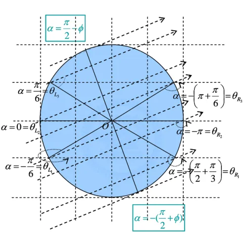
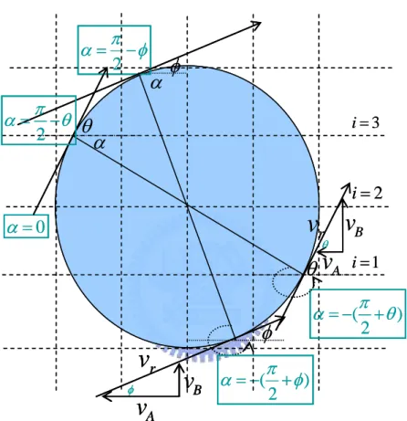
In vertical to opposite or parallel case, the relative direction between mobility nodes, MN and _A MN , is vertical. When _B MN meets a cross, it has probability of _B turning pturn and lets the relative direction become opposite or parallel. As Figure 12

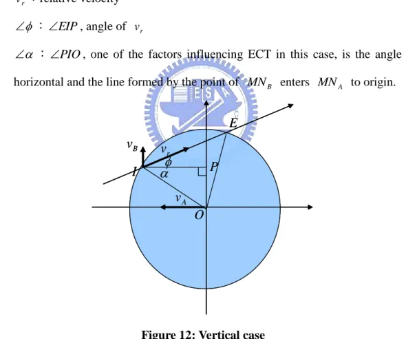
indicates relative velocity of v and _A v , and some parameters we define as _B following：

1. v ：relative velocity _r 2. ： EIP , angle of v _r

3. ：PIO, one of the factors influencing ECT in this case, is the angle of horizontal and the line formed by the point of MN enters _B MN to origin. _A

I A v E P O B v r v





I A v E P O B v r v





Figure 12: Vertical case

We reuse the partial method to calculate the ECT of vertical to opposite or parallel case in [1], for example we reuse the angle representation  to calculate the communication time. Therefore, we repeat how we get  as following

segment. [1] explained ECT can be formulated as Equation 10 if MN goes straight _B in range of MN . _A

 



























B



B v v B B B A dv d v f v t v t E v t E v T B B













    , , , , , max min 2 2         

 

  

Equation 10: ECT formulation of Vertical Case

We define mathematic symbol in Equation 11 as follow：

1. t



v_B,



：The period of MN in range of _B MN , communication time, as _A equation shows.

2. f_



v_B,



：PDF of v and _B  , as Equation 12 indicates, separated into two part, see Equation 5 and Equation 13. We explain process to get PDF of  in Equation 13 as follow segment.

3.  

2 ：Maximum value of , it also means MN will have no connection B

with MN if the _A  of MN enters the range of _B MN bigger than maximum _A value.

4. 



 



2 ： Minimum value of  , it also means MN will have no B

connection with MN if the _A  of MN enters the range of _B MN smaller than _A minimum value.































,

sin

cos

2

cos

2

,

,

2 2 B B A B A r B

v

t

v

v

v

v

R

v

R

v

t

 













Equation 11: ECT of Vertical Case



v

B



f

v



v

B

  

f

v

B

f

B

|

,





_|



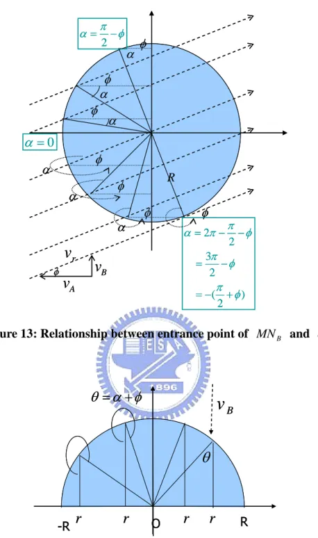
 Equation 12: PDF of v and _B  B

MN can enter range of MN from the underside of _A MN .the period from _A when MN enters the range of _B MN to when it leaves is the communication time _A we want to analyze. Nevertheless, different  causes different communication time, so we need to calculate the communication time in all possible entrance angles, multiply its corresponding PDF of v and _B  respectively to get ECT. Therefore, we analyze angle  first to get PDF of , called f

 

 . Figure 13 indicates the relation of  and entrance point of MN , and the range of B  between 



₂



and  

2 . We can observe the distance between entrance point for maximum  and minimum  is 2 , so we can express the relation of R  and r as Figure 14 shows. We can calculate CDF of f

 

 first then differentiate it to get PDF of  . Equation 13 shows process of demonstrate step by step.

     2 0 



) 2 ( 2 3 2 2                 B

v

A

v

r

v

              R      2 0 



) 2 ( 2 3 2 2                 B

v

A

v

r

v

              R

Figure 13: Relationship between entrance point of MN and _B 











-R O R B

v

r

r

r

r













-R O R B

v

r

r

r

r











 









                             _                              



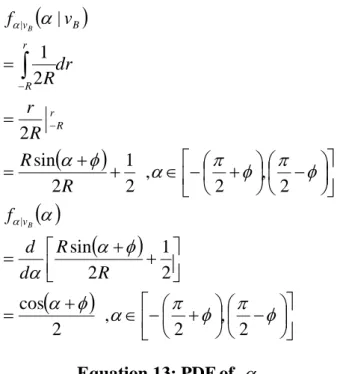
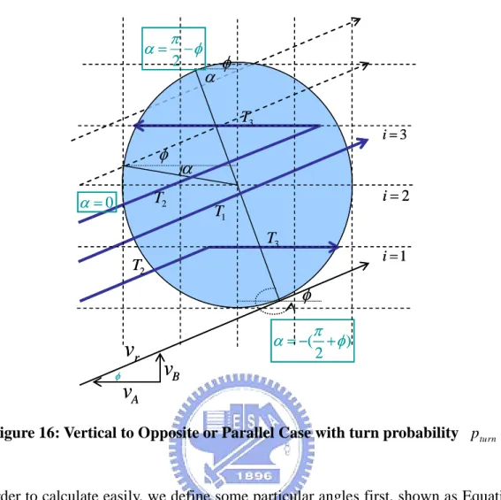
                     2 , 2 , 2 cos 2 1 2 sin 2 , 2 , 2 1 2 sin 2 2 1 | | | R R d d f R R R r dr R v f B B v r R r R B v Equation 13: PDF of 

In this thesis, MN turns with probability _B p_turn when meeting a cross and lets the direction become opposite or parallel, as Figure 15 and Figure 16 indicate. A dotted arrow represents relative direction of MN and _A MN . We divide it into two _B parts to calculate: one is that MN can’t reach some crosses and the other is that _B

B

MN can reach some crosses.

v

B

v

A

S

d

2



i

1



i

L

1



j

j



2

j



3

O R

3



i

v

B

v

A

S

d

2



i

1



i

L

1



j

j



2

j



3

O R

3



i

    2 ) 2 (    

v

_B A

v

r

v











1  i 2  i 3  i 3 T 2 T 1 T 2 T 3 T 0       2 ) 2 (    

v

_B A

v

r

v











1  i 2  i 3  i 3 T 2 T 1 T 2 T 3 T 0  

Figure 16: Vertical to Opposite or Parallel Case with turn probability pturn

In order to calculate easily, we define some particular angles first, shown as Equation 14, see the definition of symbols as follow. _Ri and _Li can be referred to Figure 17,

Hi

 can be referred to Figure 18.

1. _Ri： for intersect of number i street and right boundary of MN . _A 2. Li： for intersect of number i street and left boundary of MN . A

3. _Hi：Critical angle  that MN can reach number _B i street, means _th MN _B exactly touches i street on boundary of th MN when A MN is leaving B MN A

if MN enter range of _B MN from angle _A  . For example, if entrance angle

 is smaller than this critical angle, MN can’t reach B i street, on th the