求解p-中心的程序及決定運籌系統之p-值的方法

全文

(1)國立交通大學工業工程與管理學系碩士論文. 求解 p-中心的程序及決定運籌系統之 p-值的方法. A procedure for solving the p-center problem and determining the p value of a logistic system. 研究生：石其偉指導教授：劉復華. 教授. 中華民國九十四年八月.

(2) 求解 p-中心的程序及決定運籌系統之 p-值的方法 A procedure for solving the p-center problem and determining the p value of a logistic system. 研究生：石其偉. Student：Chi-Wei Shih. 指導教授：劉復華. Advisor：Fuh-Hwa F. Liu. 國立交通大學工業工程與管理學系碩士論文 A Thesis Submitted to Department of Industrial Engineering & Management National Chiao Tung University in partial Fulfillment of the Requirements for the Degree of Master in Industrial Engineering & Management August 2005 Hsinchu, Taiwan, Republic of China. 中華民國九十四年八月.

(3) 求解 p-中心的程序及決定運籌系統之 p-值的方法學生：石其偉. 指導教授：劉復華. 國立交通大學工業工程與管理學系碩士班. 摘. 要. 在運籌網絡之中，固定設施選址是一重要決策問題，其提供運籌系統整體的類型、結構以及形式。選址決策包括了定義供應中心的數量、位址與容量。本篇論文提出求解 p-中心問題的新程序。根據 p-中心問題的解答所做出的系統設計是一個可供考量的選擇。我們針對每一個選擇計算出八項指標，包括了最短之最遠距離、每項貨物之平均運送距離及其變異係數、每顧客端之平均運送距離及其變異係數、總固定設置成本、以及取決於各中心容量之兩項成本：變動建設成本與運輸成本。我們評估具備這八項指標之所有可能選項。數個柏拉圖有效率之選項將被選出。關鍵字：p-中心、運籌管理、服務水準、多目標、資料包絡分析法、整數規劃、柏拉圖有效率. i.

(4) A procedure for solving the p-center problem and determining the p value of a logistic system Student: Chi-Wei Shih Advisor: Fuh-Hwa F. Liu Department of Industrial Engineering & Management National Chiao Tung University ABSTRACT Locating fixed facilities throughout the logistics network is an important decision problem that gives form, structure and shape to the entire logistics system. Location decisions involve determining the number, locations and capacities of the supply centers to be used. The paper presents a new procedure to solve the minimax problem or p-center problem. The system design according to the solutions of the p-center problem is an alternative under selection. We compute the eight parameters for each alternative such as the minimax distance, average and coefficient of variation of transportation distance per unit of goods, average and coefficient of variation of transportation distance per site, the total fixed setup cost for the centers, and the two total costs that depend on the capacity of the centers: variable construction cost and transportation cost. All the possible alternatives with the eight parameters are evaluated. Several Pareto-efficient alternatives would be selected. Keywords: p-center, Logistics Management, Service Level, Multiple Criteria, Data Envelopment Analysis, Integer Programming, Pareto-Efficient. ii.

(5) 誌謝首先最感謝的是指導教授劉復華教授，在劉教授悉心的指導帶領及豐富的經驗傳承之下，給予本人極大的協助和收穫，並使我能突破研究所面臨的問題瓶頸。口試期間，更承蒙清華大學工業工程學系許棟樑副教授及本系陳文智助教授提供寶貴的意見，使本論文的內容更加嚴謹。其次要感謝的是諸位同窗和學長姐的協助與鼓勵，也要感謝我的父母親石世忠與鄭春美不時的教誨。最後願將這份論文完成的喜悅，與所有幫助過我的人一起分享。. 學生石其偉謹誌于交通大學工業工程與管理學系民國九十四年八月. iii.

(6) 目錄中文摘要............................………………………………………………………i 英文摘要............................…………………………………………….………. ii 誌謝..................................………………………………………………………iii 目錄.................................…..………………………………………………….. iv 表目錄...................………………………………………………………………v 1. Introduction............……………………………………………………….. 1 2. The modified formulation (PC-SC2) and the efficient exact procedure…...3 3. Computational results for p-SBsearch………………………………….......7 4. The allocation of the p-center problem………………………………..…..12 5. Computing throughout the M p-center problems………………...………..17 6. Determining the p value.………………………………………..…………18 7. Conclusion and discussion……………………………………………...…26 Acknowledgments…………………………………………………………......27 References..........…………………………………………………………........28. iv.

(7) 表目錄 Table 1. Results of 40 OR-Lib instances.............................................................8. Table 2. Results of TSPLIB instances...............................................................10. Table 3. Results of Random Instances...............................................................11. Table 4. Distance between 20 Sites...................................................................13. Table 5. Design parameters for each site...........................................................14. Table 6. Allocation to the nearest center and the total variable cost.................15. Table 7. New allocation with minimum cost and the lower total cost...............16. Table 8. Results of solving the p-center problems and the related index..........20. Table 9. The optimal solution of (DP1) and (DP2) and the contribution..........23. Table 10. Results of (PI2)..................................................................................24. v.

(8) 1. Introduction. Locating fixed facilities throughout the logistics network is an important decision problem that gives form, structure and shape to the entire logistics system. Location decisions involve determining the number, location and capacity of the supply centers to be used. We consider the location problem to determine the number of supply centers required to serve all the customers with minimum coverage distance. Each potential site has the variable cost to the capacity. The location and demand of each customer are given. The cost to transport a unit of demand from a potential site to each customer depends on the method employed. Location theory was first formally introduced by Alfred Weber (1909), who considered the problem of locating a single warehouse to minimize the total travel distance between the warehouse and a set of spatially distributed customers. The traditional p-center problem is to select the centers under the given p value. However, the decision maker may be incapable of determining the appropriate p value before solving the p-center problem. Considering the multiple criteria such as distance, cost, and service level, the decision maker is hard to determine the p value and select p centers with multiple objectives simultaneously. After solving the M p-center problems, we could obtain the minimax distance, allocation, cost level, and service level of all the M p-center problems. With the prior information, the decision maker could evaluate the multiple criteria to determine the appropriate p value. In Section 2, we introduce an efficient exact procedure for solving the set-covering-based p-center problem that is inspired by BsearchEx (Elloumi et al., 2004). We present our new efficient exact procedure, a slim bisecting search, called as p-SBsearch. Our new mixed-integer programming formulation (PC-SC2) is embedded in p-SBsearch to improve the solution. In Section 3, we present computational results of symmetric p-center problems with p-SBsearch and make comparison with other past research. In Section 4, we present a. 1.

(9) mixed-integer programming formulation for allocating customers to the centers with minimum total cost. Furthermore, in Section 5 we show an efficient procedure to compute throughout the M p-center problems. The system design according to the solutions of each p-center problem is an alternative under selection. We compute the eight parameters for each alternative such as the minimax distance, average and coefficient of variation of transportation distance per unit of goods, average and coefficient of variation of transportation distance per site, the total fixed setup cost for the centers, and the two total costs that depend on the capacity of the centers: variable construction cost and transportation cost. In Section 6, we evaluate the M alternatives with the eight parameters. Several Pareto-efficient alternatives would be selected. Conclusions are outlined in Section 7.. 2.

(10) 2. The modified formulation (PC-SC2) and the efficient exact procedure. Facility location models can be classified under four main topics, see Owen and Daskin (1998): z. p-center problem: it minimizes the maximum distance between any customer and its nearest center.. z. p-median problem: it minimizes the average (total) distance between customers and centers.. z. Location Set Covering Problem: it locates the least number of centers that are required to cover all customers.. z. Maximum Covering Location Problem: it seeks the maximal coverage with a given number of centers. Let N be the number of customers, M be the number of potential sites or facilities, and dij. be the distance from customer i to facility j. The p-center problem consists of locating p centers and assigning each customer to its closest center so as to minimize the maximum distance between a customer and the center it is assigned to. The location of emergency service facilities such as hospitals or fire stations is frequently modeled by the p-center problem; see Daskin (1995) and Marinov and ReVelle (1995). The p-center problem is NP-hard; see Kariv and Hakimi (1979) and Masuyama et al. (1981). Many authors consider the particular case where the facilities are identical to the customers, i.e., N=M, and distances are symmetric and satisfy triangle inequalities. We call this particular case the symmetric p-center problem. Main mathematical location methods may be categorized as heuristic and exact. Exact methods refer to those procedures with the capability to guarantee either a mathematically optimum solution to the location problem or at least a solution of known accuracy, see Drezner (1984), Handler (1990) and Daskin (1995). In many respects, this is an ideal. 3.

(11) approach to the location problem; however, the approach can result in long computer running times, huge memory requirements, and a compromised problem definition when applied to practical problems. Heuristics can be referred to as any principles or concepts that contribute to reducing the average time to search for a solution, see Chandrasekaran and Tamir (1982), Drezner (1984) and Pelegrin (1991). Although heuristic methods do not guarantee that an optimum solution has been found, the benefits of reasonable computer running times and memory requirements, good representations of reality and a satisfactory solution quality are reasons to consider the heuristic approach to warehouse location. The formulation (PC-SC) due to BsearchEx (Elloumi et al., 2004) is to solve the p-center problem, which is based on its well-known relation to the set-covering problem, by using a polynomial algorithm for computing a tighter lower bound and then solving the exact solution method. In that paper, the authors show that its linear programming relaxation provides a lower bound tighter than the classical p-center (PC) formulation, the lower bound can be computed on polynomial time, their method outperforms the running time of other recent exact methods by an order of magnitude, and it is the first one to solve large instances of size up to N=M=1817. Though the formulation (PC-SC) performs better than does formulation (PC) for given values of the lower bound and the upper bound, it is hard to solve the large scale problem by directly solving (PC-SC) within reasonable time limit. The authors proposed two algorithms to obtain the optimal solution, with complex programming procedure, complicated heuristics, and difficult concept in linear programming such as reduced cost. In this paper, we introduce a modified formulation (PC-SC2) and an easier repeating procedure, p-SBsearch, to transform a large scale problem into several small scale problems, and then obtain the optimal solution within reasonable time limit.. 4.

(12) Let Dmin = D0 < D1 < D2 < … < DK-1 < DK = Dmax be the sorted different values in the distance matrix. The formulation (PC-SC2) is the following: (PC-SC2) min z k. s.t.. (1). M. ∑y j =1. zk +. j. = p;. ∑y. (2) j. ≥ 1, i = 1,2,..., N ;. (3). j:d ij < D k. z k ∈ {0,1};. (4). y j ∈ {0,1}, j = 1,2,..., M. (5). where yj and zk are binary decision variables. Let the superscript “*” denotes the optimal *. *. solution of the decision variable. yj =1 if and only if facility j is open, and zk =0 only if it is possible to choose p centers and cover all the customers i within the radius Dk-1. Constraint (2) *. limits the number of centers to p; constraints (3) mean that, for a given k, zk =0, if and only if all customers can be served at a distance strictly lower than Dk. In the optimal solution of (PC-SC2), note that zk = 0 implies zk+1 = zk+2 = …= zK = 0. *. *. Similarly, zk = 1 implies zk-1 = zk-2 = … = z1 =1. zk = 1 and z(k+1) = 0 implies the optimal min-max value Δp* is the exact solution of the p-center problem. The integer programming problem (PC-SC2) needs at least (√2)M+1 linear programming problem (Sierksma G., 2002). Contrast to the (PC-SC) with KN+1 constraints and M+K binary variables, there are just N+1 constraints and M+1 binary variables in (PC-SC2). For the small case with M=N=100 and K=5000, the problem size of (PC-SC2) is about 250000 times smaller than the problem size of (PC-SC). (PC-SC2) is embedded in the proposed bisecting search procedure p-SBsearch that at most O(log2(MN)) recursions. Given the p value, by executing the p-SBsearch procedure one *. would obtain the optimal solution Δp* that is equal to DLp . DL and DU are respectively updated lower and upper bounds in each recursion in searching the optimal solution.. 5.

(13) Step 1 is using the bisecting search method to decide the value of k. Step 2 is performing (PC-SC2) to obtain the preliminary optimal solution zk. Step 3 is performed to check the p-center problem optimality of the current solution zk. Until reaching the optimality, we continue to solve (PC-SC2) with updating the upper bound DU and the lower bound DL. p-SBsearch Initialization: given p, D0, …, DK, set L = 0, U = K and Δp* = DU Step 1.. k=⎣(L+U)/2⎦.. Step 2.. Solving (PC-SC2) with Dk to obtain the optimal solution zk*.. Step 3.. If zk*=1, then let L=k,. Step 3.1. If zk+1=0, then STOP, set Δp* =DL, Lp*=L and Up*=U; else, goto step 1; else If zk=0, then let U=k, Step 3.2. If zk-1=1, then STOP, set Δp* =DL, Lp*=L and Up*=U; else, goto step 1.. 6.

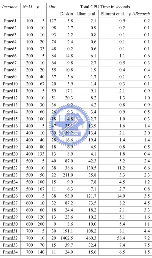
(14) 3. Computational Results for p-SBsearch. We use a notebook with 512 MB of RAM and Intel P-M 1.30 GHz of CPU. The p-SBsearch procedure was implemented with the code written by C++ and the MIP solver of CPLEX 7.1. We set the time limit parameters of MIP solver to 3600, so the solution of sub-problem stops if no integer solution is found after one hour of CPU time. We report the computational results obtained with p-SBsearch on OR-Lib (Beasley 1990) p-median and TSP-Lib (Reinelt 1991) instances. We also make comparison of p-SBsearch with Daskin (2000), Ilhan et al. (2001) and Elloumi et al. (2004). Daskin (2000) performed a binary search based on solving the maximal covering problem; Ilhan et al. (2001) proposed a two-phase algorithm with solving the IP feasibility problems; Elloumi et al. (2004) presented (PC-SC) and a resolution method based on the set-covering problem. The results of the comparison on 40 OR-Lib p-median instances are given in Table 1. The first three columns characterize the instance, and the optimal radius is in column 4. Columns 5 through 7 report the CPU time of Daskin (2000), Taylan et al. (2001) and Elloumi et al. (2004). Column 8 gives the CPU time of p-SBsearch. Even if it is not straightforward to compare CPU time on different machines, we can show the maximum and the average CPU time as indication in Table 1. Furthermore, we calculate the Coefficient of Variation (CV) to compare the computing stability with the increasing p value. The Coefficient of Variation is the standard deviation σ divided by the mean μ.. 7.

(15) Table 1 Instance. N=M. p. Results of 40 OR-Lib instances. Opt. Total CPU Time in seconds Daskin Ilhan et al. Elloumi et al. p-SBsearch. Pmed1. 100. 5. 127. 5.8. 2.1. 0.9. 0.2. Pmed2. 100. 10. 98. 2.7. 0.9. 0.2. 0.1. Pmed3. 100. 10. 93. 2.2. 0.8. 0.1. 0.1. Pmed4. 100. 20. 74. 2.4. 0.6. 0.1. 0.1. Pmed5. 100. 33. 48. 0.2. 0.6. 0.1. 0.1. Pmed6. 200. 5. 84. 14.8. 6.1. 1.1. 0.6. Pmed7. 200. 10. 64. 9.8. 2.7. 0.5. 0.3. Pmed8. 200. 20. 55. 10.8. 1.9. 0.4. 0.4. Pmed9. 200. 40. 37. 3.6. 1.7. 0.1. 0.3. Pmed10. 200. 67. 20. 3.9. 1.4. 0.3. 0.1. Pmed11. 300. 5. 59. 17.1. 9.1. 2.1. 0.9. Pmed12. 300. 10. 51. 20.3. 8.2. 1.3. 1.0. Pmed13. 300. 30. 36. 9.2. 4.2. 0.8. 0.9. Pmed14. 300. 60. 26. 9.3. 3.4. 0.9. 0.5. Pmed15. 300. 100. 18. 4.8. 2.7. 1.0. 0.3. Pmed16. 400. 5. 47. 35.1. 13.9. 1.6. 1.4. Pmed17. 400. 10. 39. 39.2. 13.4. 2.1. 2.0. Pmed18. 400. 40. 28. 16.6. 19.4. 1.4. 1.4. Pmed19. 400. 80. 18. 6.9. 4.9. 0.8. 0.5. Pmed20. 400. 133. 13. 8.9. 4.1. 1.8. 0.4. Pmed21. 500. 5. 40. 87.0. 42.3. 5.2. 2.4. Pmed22. 500. 10. 38. 38.6. 130.5. 11.2. 6.6. Pmed23. 500. 50. 22. 211.0. 35.8. 3.3. 2.3. Pmed24. 500. 100. 15. 9.9. 7.8. 4.5. 1.2. Pmed25. 500. 167. 11. 6.3. 7.1. 2.7. 0.8. Pmed26. 600. 5. 38. 93.9. 121.7. 14.9. 3.5. Pmed27. 600. 10. 32. 87.2. 73.5. 8.2. 4.5. Pmed28. 600. 60. 18. 24.4. 18.2. 2.1. 3.3. Pmed29. 600. 120. 13. 23.6. 10.2. 5.1. 1.6. Pmed30. 600. 200. 9. 8.6. 10.0. 5.4. 1.1. Pmed31. 700. 5. 30. 191.1. 108.2. 8.1. 4.4. Pmed32. 700. 10. 29 1402.5. 460.3. 58.4. 7.2. Pmed33. 700. 70. 15. 39.7. 32.4. 7.4. 7.5. Pmed34. 700. 140. 11. 24.9. 15.6. 6.5. 1.5. 8.

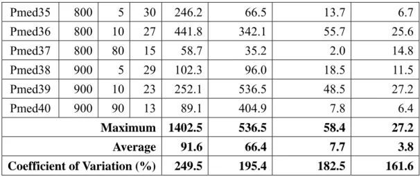
(16) Pmed35. 800. 5. 30. 246.2. 66.5. 13.7. 6.7. Pmed36. 800. 10. 27. 441.8. 342.1. 55.7. 25.6. Pmed37. 800. 80. 15. 58.7. 35.2. 2.0. 14.8. Pmed38. 900. 5. 29. 102.3. 96.0. 18.5. 11.5. Pmed39. 900. 10. 23. 252.1. 536.5. 48.5. 27.2. Pmed40. 900. 90. 13. 89.1. 404.9. 7.8. 6.4. Maximum 1402.5. 536.5. 58.4. 27.2. Average. 91.6. 66.4. 7.7. 3.8. Coefficient of Variation (%). 249.5. 195.4. 182.5. 161.6. Table 2 gives the results for TSPLIB instances and makes comparison of p-SBsearch with Elloumi et al. (2004). The first three columns characterize the instance. Columns 4 through 8 give the results of algorithm Bsearch and BsearchEx (2004). Columns LB* and UB* give the lower bound and upper bound obtained by Bsearch, and Column cpu1 is the CPU time devoted to Bsearch. Column Opt gives the optimal solution or the best found solution obtained by BsearchEx, and Column cpu2 is the CPU time devoted to BsearchEx. Columns 9 through 12 give the results of p-SBsearch. There is tradeoff between solution time and the preciseness of solution in large scale problems. Based on the update of max and min of p-SBsearch, we could set the bound tolerance in advance to obtain a narrow solution bound in shorter CPU time. If the relative bound tolerance (Dmax-Dmin)/Dmin does not exceed 5% for any sub-problem, we stop p-SBsearch and record the current bound. Column 5% Bound gives the results of 5% bound tolerance, and Column cpu3 is the CPU time of 5% bound tolerance. Column Opt2 gives the results of p-SBsearch, and Column cpu4 is the CPU time of our p-SBsearch procedure. If the optimal solution is not reached in an hour, set zk = 1 and L = k to solve the next sub-problem. When this happens we are no longer sure that our solution is optimal, and then we give the best solved bound in Column Opt2.. 9.

(17) Table 2 Instance. N=M. Results of TSPLIB instances. Elloumi et al.. p. p-SBsearch. LB*. UB*. Opt. cpu1. cpu2. 5% Bound. Opt2. cpu3. cpu4. u1060. 1060. 10. 2273. 2273. 2273. 27. 53. 2272-2386. 2273. 36. 52. u1060. 1060. 20. 1556. 1768. 1581. 63. 2778. 1531-1590. 1581. 135. 2329. u1060. 1060. 30. 1205. 1275. 1208. 50. 298. 1185-1210. 1208. 36. 257. u1060. 1060. 40. 1013. 1079. 1021. 35. 366. 1005-1029. 1021. 26. 121. u1060. 1060. 50. 895. 963. 905. 21. 383. 905-921. 905. 191. 273. u1060. 1060. 60. 765. 807. 781. 21. 233. 761-790. 781. 4. 437. u1060. 1060. 70. 707. 761. 711. 17. 135. 708-738. 710* (708-721). 7. 3608. u1060. 1060. 80. 652. 711. 652. 18. 60. 640-670. 652. 2. 8. u1060. 1060. 90. 604. 636. 608. 19. 38. 600-609. 608. 2. 6. u1060. 1060. 100. 570. 570. 570. 18. 29. 570-599. 570. 1. 2. u1060. 1060. 110. 539. 539. 539. 18. 30. 538-552. 539. 1. 1. u1060. 1060. 120. 510. 538. 510. 29. 44. 510-515. 510. 3. 3. u1060. 1060. 130. 495. 510. 500. 28. 44. 495-510. 500. 1. 3. u1060. 1060. 140. 452. 500. 452. 28. 46. 452-474. 452. 1. 2. u1060. 1060. 150. 430. 447. 447. 34. 50. 447-452. 447. 1. 1. rl1323. 1323. 10. 3062. 3329. 3077. 106. 1380. 3017-3155. 3077. 62. 265. rl1323. 1323. 20. 2008. 2152. 2016. 115. 480. 1949-2036. 2016. 97. 2543. rl1323. 1323. 30. 1611. 1797. 1632. 99. 900. 1587-1640. 1632. 193. 5147. *. rl1323. 1323. 40. 1334. 1521. 1352. 76. 3000. 1339-1381. 1365 (1339-1366) 3233. 14132. rl1323. 1323. 50. 1165. 1300. 1187. 61. 8580. 1164-1197. 1187* (1164-1188) 156. 14571. *. rl1323. 1323. 60. 1047. 1194. 1063. 55. 9120. 1048-1076. 1066 (1048-1067) 23. 13382. rl1323. 1323. 70. 959. 1040. 972. 42. 1740. 970-1018. 980* (872-981). 3603. 16665. rl1323. 1323. 80. 889. 948. 895. 37. 420. 894-936. 903* (805-904). 3603. 18116. *. rl1323. 1323. 90. 830. 857. 832. 30. 120. 824-864. 834 (832-835). 3. 7503. rl1323. 1323. 100. 777. 803. 787. 26. 120. 763-796. 788* (779-789). 145. 8645. u1817. 1817. 10. 455. 467. 458. 611. 2700. 457-480. 458. 789. 3973. u1817. 1817. 20. 306. 342. 310*. 660. 4920. 306-318. 314* (306-315). 937. 8499. *. *. u1817. 1817. 30. 240. 287. 250. 355. 16500. 251-257. 251 (232-252). 7718. 8321. u1817. 1817. 40. 205. 234. 210*. 247. 6420. 211-221. 216* (169-217). 4344. 9049. u1817. 1817. 50. 180. 205. 187*. 242. 9840. 183-190. 189* (145-190). 4287. 15087. u1817. 1817. 60. 163. 183. 163. 177. 1260. 162-169. 162. 175. 348. u1817. 1817. 70. 148. 152. 148. 166. 420. 143-149. 148. 82. 106. 10.

(18) u1817. 1817. 80. 137. 148. 137. 150. 1140. 142-148. 137* (127-140). 3696. 3814. u1817. 1817. 90. 127. 148. 130*. 161. 7202. 127-131. 130* (127-131). 96. 7296. u1817. 1817. 100. 127. 130. 127. 159. 300. 126-130. 127* (126-128). 13. 3670. u1817. 1817. 110. 108. 127. 109. 119. 420. 109-111. 109. 181. 453. u1817. 1817. 120. 108. 108. 108. 131. 120. 107-109. 108. 12. 18. *. *. u1817. 1817. 130. 105. 109. 108. 121. 3720. 105-108. 107 (99-108). 3605. 7212. u1817. 1817. 140. 102. 108. 105*. 121. 4020. 102-107. 105* (97-107). 3606. 7212. u1817. 1817. 150. 92. 108. 94*. 144. 5640. 99-102. 99* (89-102). 7256. 7256. *. Note. “ ” = opt2 is the best found solution for that instance. The range in brackets is the best-solved value of p-SBsearch. Columns cpu1, cpu2, cpu3 and cpu4 are recorded in seconds.. Finally, as Elloumi et al. (2004), we generated a few random Euclidean instances and random instances with N=M=100, p=5, 10, 15. In the random Euclidean instances Euc100, coordinates of the points are randomly generated in [0, 100]; and Euclidean distances are computed between the points. In the random instances Rand100, distances are randomly and uniformly generated in [0, 100] and satisfy dij = 0 and dij = dji. Table 3 reports the results obtained for these instances.. Table 3. Results of Random Instances. Instance. N=M p. Opt. cpu (in seconds). Euc100. 100. 5. 32. 0.1. Euc100. 100. 10. 20. 0.1. Euc100. 100. 15. 16. 0.1. Rand100 100. 5. 27. 13.2. Rand100 100. 10. 12. 9.3. Rand100 100. 15. 7. 1.4. 11.

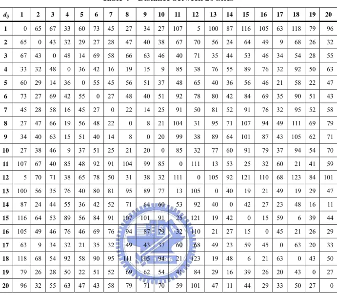
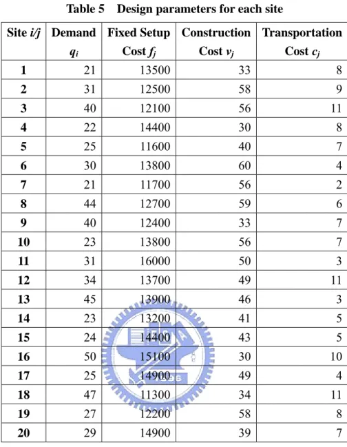
(19) 4. The allocation of the p-center problem. The formulation (PC-SC2) does not give the allocation of the customers in an explicit way. In the p-center problem, one may determine the assignment of customer i to the closest center by looking for center jo (Elloumi et al., 2004) such that d ijo = min j: y * =1 d ij. (6). j. We propose a minimum total cost model (MTC) for the allocation problem to the selected p centers. Suppose the i-th customer has a demand of qi. Let xij = 1 if we assign the customer i to the center j and the cost to increase the capacity for each additional unit of goods is vj. The cost to transport a unit of goods for a unit distance from center j, denoted as cj, depends on the transportation method which is employed. One may solve the following model to determine the allocation of the p-center problem: (MTC) min. ∑. vj. j : y *j =1. s.t.. ∑x. ∑q x. i ij. i:d ij ≤ Δ*p. ij. +. ∑. cj. j : y *j =1. ∑q d. x. (7). i ij ij. i:d ij ≤ Δ*p. = 1, i : d ij ≤ Δ*p ;. (8). j: y *j =1. xij ∈ {0,1}, i : dij ≤ Δ*p , j : y*j = 1.. (9). Constraints (8) limit the customer i to be assigned to only one center. After minimizing the total cost for the system with p centers, one could obtain the allocation Ej, the set of customers assigned to the center j. We use a set of data for illustration. There are 20 potential sites, and we want to select 3 of them to be distribution centers. Distance between sites, demand of each site, fixed setup cost, and the variable cost to each center are given as follows:. 12.

(20) Table 4 dij. 1. Distance between 20 Sites. 2. 3. 4. 5. 6. 7. 8. 9. 10. 11. 12. 13. 14. 15. 16. 17. 18. 19. 20. 1. 0. 65. 67. 33. 60. 73. 45. 27. 34. 27. 107. 5. 100. 87. 116. 105. 63. 118. 79. 96. 2. 65. 0. 43. 32. 29. 27. 28. 47. 40. 38. 67. 70. 56. 24. 64. 49. 9. 68. 26. 32. 3. 67. 43. 0. 48. 14. 69. 58. 66. 63. 46. 40. 71. 35. 44. 53. 46. 34. 54. 28. 55. 4. 33. 32. 48. 0. 36. 42. 16. 19. 15. 9. 85. 38. 76. 55. 89. 76. 32. 92. 50. 63. 5. 60. 29. 14. 36. 0. 55. 45. 56. 51. 37. 48. 65. 40. 36. 56. 46. 21. 58. 22. 47. 6. 73. 27. 69. 42. 55. 0. 27. 48. 40. 51. 92. 78. 80. 42. 84. 69. 35. 90. 51. 43. 7. 45. 28. 58. 16. 45. 27. 0. 22. 14. 25. 91. 50. 81. 52. 91. 76. 32. 95. 52. 58. 8. 27. 47. 66. 19. 56. 48. 22. 0. 8. 21. 104. 31. 95. 71. 107. 94. 49. 111. 69. 79. 9. 34. 40. 63. 15. 51. 40. 14. 8. 0. 20. 99. 38. 89. 64. 101. 87. 43. 105. 62. 71. 10. 27. 38. 46. 9. 37. 51. 25. 21. 20. 0. 85. 32. 77. 60. 91. 79. 37. 94. 54. 70. 11. 107. 67. 40. 85. 48. 92. 91. 104. 99. 85. 0. 111. 13. 53. 25. 32. 60. 21. 41. 59. 12. 5. 70. 71. 38. 65. 78. 50. 31. 38. 32. 111. 0. 105. 92. 121. 110. 68. 123. 84. 101. 13. 100. 56. 35. 76. 40. 80. 81. 95. 89. 77. 13. 105. 0. 40. 19. 21. 49. 19. 29. 47. 14. 87. 24. 44. 55. 36. 42. 52. 71. 64. 60. 53. 92. 40. 0. 42. 27. 23. 48. 16. 11. 15. 116. 64. 53. 89. 56. 84. 91. 107. 101. 91. 25. 121. 19. 42. 0. 15. 59. 6. 39. 44. 16. 105. 49. 46. 76. 46. 69. 76. 94. 87. 79. 32. 110. 21. 27. 15. 0. 45. 21. 26. 29. 17. 63. 9. 34. 32. 21. 35. 32. 49. 43. 37. 60. 68. 49. 23. 59. 45. 0. 63. 20. 33. 18. 118. 68. 54. 92. 58. 90. 95. 111. 105. 94. 21. 123. 19. 48. 6. 21. 63. 0. 43. 50. 19. 79. 26. 28. 50. 22. 51. 52. 69. 62. 54. 41. 84. 29. 16. 39. 26. 20. 43. 0. 27. 20. 96. 32. 55. 63. 47. 43. 58. 79. 71. 70. 59. 101. 47. 11. 44. 29. 33. 50. 27. 0. 13.

(21) Table 5. Design parameters for each site. Site i/j Demand Fixed Setup Construction Transportation qi Cost fj Cost vj Cost cj 1. 21. 13500. 33. 8. 2. 31. 12500. 58. 9. 3. 40. 12100. 56. 11. 4. 22. 14400. 30. 8. 5. 25. 11600. 40. 7. 6. 30. 13800. 60. 4. 7. 21. 11700. 56. 2. 8. 44. 12700. 59. 6. 9. 40. 12400. 33. 7. 10. 23. 13800. 56. 7. 11. 31. 16000. 50. 3. 12. 34. 13700. 49. 11. 13. 45. 13900. 46. 3. 14. 23. 13200. 41. 5. 15. 24. 14400. 43. 5. 16. 50. 15100. 30. 10. 17. 25. 14900. 49. 4. 18. 47. 11300. 34. 11. 19. 27. 12200. 58. 8. 20. 29. 14900. 39. 7. In the optimal solution of p-Sbsearch, we select sites 1, 2 and 13 to be distribution centers with minimax distance Δp* = 35. One may determine the allocation of each customer by (6). The results of the allocation and the cost are shown in Table 6.. 14.

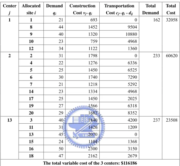
(22) Table 6. Allocation to the nearest center and the total variable cost. Center j. Allocated site i. 1. 1. 21. 693. 0. 8. 44. 1452. 9504. 9. 40. 1320. 10880. 10. 23. 759. 4968. 12. 34. 1122. 1360. 2. 31. 1798. 0. 4. 22. 1276. 6336. 5. 25. 1450. 6525. 6. 30. 1740. 7290. 7. 21. 1218. 5292. 14. 23. 1334. 4968. 17. 25. 1450. 2025. 19. 27. 1566. 6318. 20. 29. 1682. 8352. 3. 40. 1840. 4200. 11. 31. 1426. 1209. 13. 45. 2070. 0. 15. 24. 1104. 1368. 16. 50. 2300. 3150. 18. 47. 2162. 2679. 2. 13. Demand qi. Construction Cost vj* qi. Transportation Cost cj* qi * dij. Total Demand. Total Cost. 162. 32058. 233. 60620. 237. 23508. The total variable cost of the 3 centers: $116186. If we revise the allocation by solving the allocation model (MTC), we obtain the new allocation and the lower total cost in Table 7. The difference between original allocation and new allocation is that we assign site 4 to be served by center 1 instead of center 2, and site 19 to be served by center 13 instead of center 2. The reason for site 4 and 19 not to be assigned to center 2 is that the variable cost v2 and c2 are the largest among the three centers. Though the assigned distance increases, we could save $5371 in the total cost and still keep the minimum radius at the same time.. 15.

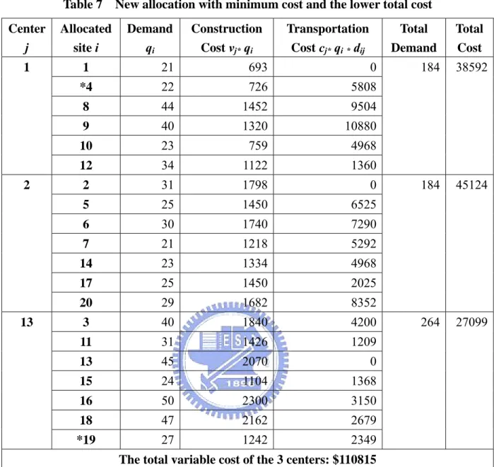
(23) Table 7. New allocation with minimum cost and the lower total cost. Center j. Allocated site i. 1. 1. 21. 693. 0. *4. 22. 726. 5808. 8. 44. 1452. 9504. 9. 40. 1320. 10880. 10. 23. 759. 4968. 12. 34. 1122. 1360. 2. 31. 1798. 0. 5. 25. 1450. 6525. 6. 30. 1740. 7290. 7. 21. 1218. 5292. 14. 23. 1334. 4968. 17. 25. 1450. 2025. 20. 29. 1682. 8352. 3. 40. 1840. 4200. 11. 31. 1426. 1209. 13. 45. 2070. 0. 15. 24. 1104. 1368. 16. 50. 2300. 3150. 18. 47. 2162. 2679. *19. 27. 1242. 2349. 2. 13. Demand qi. Construction Cost vj* qi. Transportation Cost cj* qi * dij. Total Demand. The total variable cost of the 3 centers: $110815 (*): The different allocation between Table 6 and 7. 16. Total Cost. 184. 38592. 184. 45124. 264. 27099.

(24) 5. Computing throughout the M p-center problems. The p-center problem consists of locating p centers among the M potential facilities and assigning each customer to its closest center so as to minimize the maximum distance between a customer and the center it is assigned to. For a logistic system design purpose, one may need to obtain the solutions for all the M p-center problems where p alternatively equals to 1, 2, throughout M. Given the p value, the parameters yj* and Ej are determined by employing p-SBsearch procedure. The procedure proposed in this paper also has the advantage for computing throughout the M p-center problems. There are three possible solving strategies. The first strategy is to employ p-SBsearch procedure to solve the problems with larger p, say pa-center problem where pa > p. The pa-SBsearch procedure is identical to the p-SBsearch procedure except in the initialization step setting U=Up* in the preceding problem. One may solve the problems one after the other, p=1, 2, 3, …, M. The second strategy is to employ p-SBsearch procedure to solve the problems with smaller p, say pb-center problem where pb < p. The pb-SBsearch procedure is identical to the p-SBsearch procedure except in the initialization step setting L=Lp* in the preceding problem. One may solve the problems one after the other, p=M, M-1, …, 3, 2, 1. The third computation strategy is initiated by employing p-SBsearch procedure for p=1 and pa-SBsearch procedure for p=M. Then, alternate with pb-SBsearch and pa-SBsearch to solve the problems with p values (2, M-1), (3, M-3), …, (M/2) in turns, repsectively. In each turn, L=Lp* or U=Up* is updated for the p-SBsearch procedure. Apparently, the number of sub-problems in pa-SBsearch and pb-SBsearch are less than p-SBsearch and the global optimal solution still reached. Without starting from L=0 and U=K to every p value, savings in computation time for the three strategies are benefited.. 17.

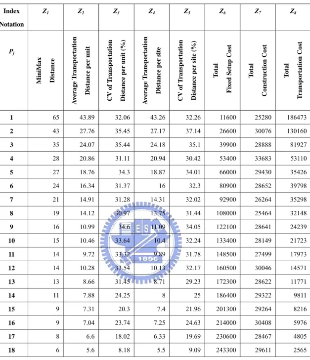
(25) 6. Determining the p value. The traditional p-center problem assumes that the decision maker has determined the parameter p. In the real-world case, however, the decision maker may be incapable of determining the appropriate p value before solving the p-center problem. In a logistic system, one may consider the minimax condition of the p-center problem and the fixed setup cost, variable construction cost for the supplier centers, the transportation cost and the service level for the designed system as well. The service level for a logistic system may be interpreted varieties factors such response time of the demand, shortage of goods and cost to maintain the service level, etc (refer to the text book by Ballou). In this research we chose eight parameters to measure the logistic system design alternatives. The criteria should not be limited. We use the same data in Section 4 to illustrate how to determine the p value for the logistic system. First, after solving the M p-center problems by the p-SBsearch procedure and the allocation model (MTC), the results are shown in Table 8. Note that we does not solve the problems with p = 19 and 20 because there are zero value in x1, x3, or x5, and it is irrational to select almost all the sites to be centers for the general p-center problem. Column Z1 denotes the optimal solution Δp* of the p-SBsearch procedure. Columns Z2 to Z5 characterize the service level of the system. We ignore the demand while the assigned distance dij = 0 to obtain the appropriate average transportation distance and CV. Column Z2 denotes the average transportation distance per unit, and the value increases with the larger p. z2j=. ∑ ∑q d. j: y *j =1 i: 0< d ij. i. ij. xij*. ∑ ∑q x. j: y *j =1 i: 0< dij. * i ij. (10). Column Z3 denotes the dispersion level of the transportation distance per unit, the coefficient of variation, to evaluate the stability of the service distance. Columns Z4 and Z5 consider the emergent demand of each site, so we don’t take the demand qi into account.. 18.

(26) z4j=. ∑ ∑d. j: y*j =1 i: 0< dij. * ij ij. x. ∑ ∑x. j: y*j =1 i: 0<dij. * ij. (11). Columns Z6 to Z8 characterize the cost level of the system. The total cost is divided into three part: the fixed setup cost, the construction cost, and the transportation cost. z6j=. ∑f. (12). j. j: y *j =1. z7j=. ∑ v ∑q x. (13). z8j=. ∑ c ∑q d x. (14). * i ij. j. j : y *j =1. i:d ij ≤ Δ*p. * i ij ij. j. j : y *j =1. i:d ij ≤ Δ*p. 19.

(27) Table 8. Results of solving the p-center problems and the related index. Z1. Index. Z2. Z3. Z4. Z5. Z6. Z7. Z8. Transportation Cost. Total. Construction Cost. Total. Fixed Setup Cost. Total. Distance per site (%). CV of Transportation. Distance per site. Average Transportation. Distance per unit (%). CV of Transportation. Distance. MiniMax. Pj. Distance per unit. Average Transportation. Notation. 1. 65. 43.89. 32.06. 43.26. 32.26. 11600. 25280. 186473. 2. 43. 27.76. 35.45. 27.17. 37.14. 26600. 30076. 130160. 3. 35. 24.07. 35.44. 24.18. 35.1. 39900. 28888. 81927. 4. 28. 20.86. 31.11. 20.94. 30.42. 53400. 33683. 53110. 5. 27. 18.76. 34.3. 18.87. 34.01. 66000. 29430. 35426. 6. 24. 16.34. 31.37. 16. 32.3. 80900. 28652. 39798. 7. 21. 14.91. 31.28. 14.31. 32.02. 92900. 26264. 35298. 8. 19. 14.12. 30.97. 13.75. 31.44. 108000. 25464. 32148. 9. 16. 10.99. 34.6. 11.09. 34.05. 122100. 28641. 24239. 10. 15. 10.46. 33.64. 10.4. 32.24. 133400. 28149. 21723. 11. 14. 9.72. 33.32. 9.89. 31.78. 148500. 27499. 17973. 12. 14. 10.28. 33.54. 10.13. 32.17. 160500. 30046. 14571. 13. 13. 8.66. 31.45. 8.71. 29.23. 172300. 28622. 11771. 14. 11. 7.88. 24.25. 8. 25. 186400. 29322. 9811. 15. 9. 7.31. 20.3. 7.4. 21.96. 201300. 29264. 8216. 16. 9. 7.04. 23.74. 7.25. 24.63. 214000. 30408. 5976. 17. 8. 6.6. 18.02. 6.33. 19.69. 230600. 28467. 4805. 18. 6. 5.6. 8.18. 5.5. 9.09. 243300. 29611. 2565. There are 18 possible p values for selection, p = 1, 2, …, 18. The parameter zij denotes the value of Pj in the ith index. Since these eight indices are expected to be minimum, we could set the weights vi to obtain the performance index ωj, an aggregate weighted index: 8. ω j = ∑ z ij vi. (15). i =1. However, it is hard to determine arbitrarily the appropriate weights by the decision maker. To evaluate the multiple criteria to determine the appropriate p value, we use an evaluation. 20.

(28) model (PI) inspired by the Data Envelopment Analysis (DEA) (Charnes et al., 1978) to obtain the performance value. The DEA model classifies the DMUs as efficient or inefficient (Cooper et al., 2000), based on multiple inputs and multiple outputs. The following model (PI) is employed for measuring the relative performance score, ωo of Po against the n alternatives. (PI) 8. min ω o = ∑ z io vi. (16). i =1. s.t.. 8. ∑z i =1. v ≥ 100, j = 1,2,..., n;. (17). ij i. 8. z1o v1 ≥ ∑ z io vi ;. (18). i =2. 5. 8. i=2. i =6. ∑ z io vi ≥ ∑ z io vi ;. (19). vi ≥ ε , i = 1,2,...,6.. (20). The objective function (16) is to minimize the ωo of Po, so we resolve the model with o = 1, 2, …, n. In each turn, this model determines the most favorable weights to DMUo. 8. Constraints (17) set DMUj‘s lower bound of the performance index ω j = ∑ z ij vi ≧100. Any i =1. lower bound value will not affect the final solution. Constraint (18) confirms that the contribution in the performance index by the minimax distance index, the most important condition of the p-center problem, is greater than or equal to the total contribution of the other indices. Constraint (19) confirms that the contribution in the performance index by the service level index is greater than or equal to the contribution by the cost level. In this case we assume that the service level of the system is more important than the cost level. To solve the (PI) model without setting the value of ε, we solve the following two-phase LP problem.. 21.

(29) Phase I We solve the dual model (DPI) of (PI) as follows: (DPI) n. max ηo = 100∑ λ j. (21). j =1. n. ∑z. s.t.. λ j + z1o γ 1 ≤ z1o ;. (22). λ j − z ij γ 1 + z ij γ 2 ≤ z io , i = 2,3,4,5;. (23). λ j − z ij γ 1 − z ij γ 2 ≤ z io , i = 6,7,8;. (24). 1j. j =1 n. ∑z j =1. ij. n. ∑z j =1. ij. λ j ≥ 0, j = 1,2,..., n;. (25). γ 1 ,γ 2 ≥ 0. (26). where λj, γ1 and γ2 are the corresponding dual variables to the constraints (17), (18), and (19). If the optimal solution ηo* of (DPI) is equal to 100, we solve the next model (DP2).. Phase II (DP2) max. 8. ∑s i =1. (27). i. n. s.t. 100∑ λ j = 100;. (28). j =1. n. ∑z j =1. λ j + z1o γ 1 + s1 = z1o ;. (29). ij. λ j − z ij γ 1 + z ij γ 2 + si = z io , i = 2,3,4,5;. (30). ij. λ j − z ij γ 1 − z ij γ 2 + si = z io , i = 6,7,8;. (31). 1j. n. ∑z j =1 n. ∑z j =1. λ j ≥ 0, j = 1,2,..., n;. (32) (33). γ 1 ,γ 2 ≥ 0;. si ≥ 0, i = 1,2,...,8. (34). 22.

(30) where we fix the performance index of Po and maximize the sum of all the slack variables si. Only the alternatives with ηo*=1 in (DP1) and si* = 0 for all i in (DP2) are Pareto-efficient alternatives. Table 9 shows the computational results of (DP1) and (DP2). DMU 1, 2, 4, and 18 are the Pareto-efficient alternatives with ηo* = 1 and si* = 0 for all i. To the alternatives with 1, 2, 4, or 18 centers are the appropriate choice by considering the minimax distance, the service level, and the cost level. Table 9 DMU j. The optimal solution of (DP1) and (DP2) and the contribution. η j*. z1 j v1*. z 2 j v2*. z3 j v3*. z 4 j v4*. z5 j v5*. z 6 j v6*. z 7 j v7*. z8 j v8*. ω *j. ω *j. ω *j. ω *j. ω *j. ω *j. ω *j. ω *j. 1. 100. 50%. 2. 100. 50%. 3. 104.82. 4. 100. 5. 103.70. 6. 105.13. 7. 112.29. 8. 121.79. 9. 123.00. 10. 126.61. 11. 130.22. 12. 137.09. 13. 134.15. 14. 128.75. 15. 118.62. 16. 122.49. 17. 116.82. 18. 100. 25% 13%. 12%. 8% 23%. 2% 7%. 50%. 25%. 18%. 50%. 25%. 25%. 23. 17%.

(31) If the decision maker is still incapable of determining the p value, we propose another model (PI2) to rank these efficient alternatives and to exclude the alternatives which are not robust in the adverse condition. (PI2) 8. max π o = ∑ z io vi. (35). i =1. s.t.. 8. ∑z i =1. v ≤ 100, j = 1,2,..., n;. (36). ij i. 8. z1o v1 ≥ ∑ z io vi ;. (37). i =2. 5. 8. i=2. i =6. ∑ z io vi ≥ ∑ z io vi ;. (38). vi ≥ ε , i = 1,2,...,6.. (39). We revise the bound constraints (36) to set the upper bound of the performance index 8. π j = ∑ z ij vi ≦100. The model (PI2) is to maximize the performance index and determine the i =1. most adverse weights to Po. If any Pj performs efficient with the favorable weights in (PI) and is distance from the upper bound with the adverse weights in (PI2), we assume that this kind of alternative is stable and robust in performance. The results of (PI2) are showed in Table 10.. Table 10. Results of (PI2). DMUj ωj* in (PI) πj* in (PI2) Rank 1. 100. 100. 4. 2. 100. 87.17. 3. 4. 100. 67.90. 2. 18. 100. 15.83. 1. To the decision maker, p=18 might be the best choice if we rank these alternatives by πj* in (PI2). However, all the value of the parameters in our data is artificial and unreal, and we never know the authentic relationship of importance between the minimax distance, cost level, and service level. Based on the different circumstance and the specific service or cost. 24.

(32) conditions, the decision maker could select the appropriate p value from p = 2, 4, and 18 in this case.. 25.

(33) 7. Conclusion and discussion. Our computational results are showed in the Table 1 to 3. To the OR-Lib instances with network structure, the TSPLIB instances that are usually devoted to the traveling salesman problem, the random Euclidean instances that satisfy the triangle inequalities, and the random instances for which the triangle inequalities are not satisfied, the proposed procedure p-SBsearch is efficient in the reasonable time limit and exact with good quality of the solution bounds. There may be some other considerations to allocate customers to centers for specific industry. The model presented in Section 4 could be reformulated. One may have less or more parameters for evaluating the possible alternatives. Furthermore, one may add constraints for the relationship among the parameters. Literature in the area of Data Envelopment Analysis (DEA) would be a good source for reference the multiple criteria assessment. The model presented in Section 6 is modified accordingly. The paper provides a new concept to determine the proper number of supply centers for the logistic system. Other system may have same interest for the problem settings.. 26.

(34) Acknowledgments. This research is supported by the National Science Council of Republic of China (Taiwan) under the project 93-2213-E-009-016- for two years.. 27.

(35) References. 1.. Ballou, R. H., 1992. Business Logistics Management. Prentice-Hall Inc., New Jersey.. 2.. Beasley, J. E., 1990. OR-Library: distributing test problems by electronic mail. Journal of the Operational Research Society 41, 1069-1072.. 3.. Chandrasekaran, R., Tamir, A., 1982. Polynomially bounded algorithms for locating p-centers on a tree. Mathematical Programming 22, 304-315.. 4.. Charnes, A., Cooper, W. W. and Rhodes, E., 1978. Measuring the efficiency of decision making units. European Journal of Operational Research 2, 429-444.. 5.. Cooper, W. W., Seiford L. M., Tone, K., 2000. Data Envelopment Analysis: A Comprehensive Text with Models, Applications, References and DEA-Solver Software. Kluwer Academic Publishers, Boston.. 6.. Daskin, M., 1995. Network and Discrete Location: Models, Algorithms and Applications. John Wiley and Sons, Inc., New York.. 7.. Daskin, M., 2000. A new approach to solving the vertex p-center problem to optimality: Algorithm and computational results. Communications of the Operations Research Society of Japan 45, 428-436.. 8.. Drezner, Z., 1984. The p-center problem: Heuristic and optimal algorithms. Journal of the Operational Research Society 35, 741-748.. 9.. Elloumi, S., Labbe, M., Pochet, Y., 2004. A New Formulation and Resolution Method for the p-center Problem. INFORMS Journal on Computing 16, 89-94.. 10. Handler, G. Y., 1990. p-center Problems, in Discrete Location Theory. John Wiley Inc., New York, 305-347. 11. Ilhan, T., Pinar, M., 2001. An Efficient Exact Algorithm for the Vertex p-Center Problem. http://www.optimization-online.org/. 12. Kariv, O., Hakimi, S. L., 1979. An algorithmic approach to network location problems,. 28.

(36) Part 1: The p-centers. SIAM Journal on Applied Mathematics 37, 513-538. 13. Marianov, V., ReVelle, C. S., 1995. Siting emergency services. In Drezner, Z. (ed.), Facility Location: A Survey of Applications and Methods. Springer-Verlag, New York, 199-223. 14. Masuyama, S., Ibaraki, T., Hasegawa, T., 1981. The computational complexity of the m-center problems on the plane. Transactions IECE Japan E64, 57-64. 15. Owen, S. H., Daskin, M. S., 1998. Strategic facility location: A review. Europe Journal of Operational Research 111, 423-447. 16. Pelegrin, B., 1991. Heuristic methods for the p-center problem. RAIRO Recherche Operationelle 25, 65-72. 17. Reinelt, G., 1991. TSPLIB-a travelling salesman problem library. ORSA Journal on Computing 3, 376-384. 18. Sierksma, G., 2002. Linear and Integer Programming: Theory and Practice. Marcel Dekker, Inc., New York, 326-329. 19. Weber, A., 1909. Uber den Standort der Industrien, 1. Teil: Reine Theorie Des Standortes. Tubingen, Germany.. 29.

(37)