Further study on anti-inflammatory oxygenated steroids from the octocoral Dendronephthya griffini

機差變方非均質時綜合試驗資料分析的一個新方法

陳嘉瑩

1

_、胡凱康

1

_、楊素絲

2

_、彭雲明

1

_*

1_{國立臺灣大學農藝學系} 2_{行政院農委會花蓮區農業改良場蘭陽分場}

摘要

長 久 以 來，綜 合 試 驗 資 料 均 以 傳 統 的 綜 合 變 方 分 析 的 方 式 來 分 析，這 個 分 析 的 前 提 — 機 差 均 方 需 具 有 均 質 性 — 是 大 多 數 資 料 無 法 滿 足 的 條 件。若 是 在 前 提 違 背 的 情 形 下 仍 以 傳 統 變 方 分 析 模 式 進 行 統 計 分 析，則 可 能 導 致 第 一 型 錯 誤 率 的 大 幅 偏 離 名 目 值。我 們 提 出 新 的 觀 點，目 的 在 於 放 寬 均 質 性 的 要 求，改 為 設 法 描 述 異 質 性 的 結 構，主 要 是 設 法 將 所 有 的 機 差 均 方 歸 類 為 少 數 幾 層，使 得 每 層 內 的 均 方 值 較 接 近 ， 層 數 的 多 少 是 依 據 AIC 的值來判 斷。俟 機 差 的 變 方 結 構 確 定 後，以 混 合 模 式 的 方 式 分 析 綜 合 試 驗 資 料，整 個 統 計 分 析 的 計 算 可 以 利 用 SAS 套 裝 軟 體 的 proc mixed 來 達 成 。 一 個 小 型 的 模 擬 研 究 也 說 明 了 新 的 方 法 對 控 制 第 一 型 誤 差 率 上 的 控 制 有 大 幅 的 改 善 。 關鍵詞︰綜合試驗資料、機差均質性、綜合變 方分析、第一型錯誤率、混合模式。

A New Approach to the Analysis of

Combined Experimental Data When the

Error Variances are not Homogeneous

Chia-Ying Chen1_{, Kae-Kang Hwu}1_,

Sue-S Yang2 _{and Yun-Ming Pong}1_* 1 _{Department of Agronomy, National Taiwan}

University, Taipei 10617, Taiwan ROC

2 _{Lang-yang Agricultural Experiment Station,}

Hualien District Agricultural Research and Extension, Hualien Hsien 97309, Taiwan ROC

ABSTRACT

Conventional combined analysis of variance has been employed to analyze combined field trial data for a long time. One of the assumptions of this method is about the homogeneity of error variances. However, field trial data collected by agronomists and breeders seldom meet this requirement. Since there is no alternatives while this assumption is violated and the scientists are usually forced to ignore the assumption and proceed to do the conventional combined analysis. This might end up an inflation or shrinkage of type I error rate. Instead of sticking to the unreasonable assumption, we propose a procedure for finding effective error variance structure. One out of a handful possible error variance structures will be pick as working error variance structure which has the smallest AIC value. Once the structure is determined a mixed effects model with this error structure is used to fit the data. The computation of the proposed method can be executed by SAS proc mixed. A small scale simulation study shows that the proposed method has a significant improvement over the conventional one on the control of type I error rate.

Key words: Combined experimental data,

Homogeneity of error variances, Combined analysis of variance, Type I error rate, Mixed effects models. * 通信作者, [email protected]

投 稿 日 期：2005 年 4 月 28 日 接 受 日 期：2005 年 8 月 30 日

作 物 、 環境 與生 物 資 訊 2:315-335 (2005) Crop, Environment & Bioinformatics 2:315-335 (2005) 189 Chung-Cheng Rd., Wufeng, Taichung Hsien 41301, Taiwan ROC

傳統綜合試驗資料分析之回顧

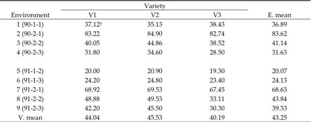
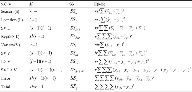
綜 合 試 驗 資 料 之 分 析 傳 統 上 均 採 用 綜 合變方分析(combined analysis of variance)，這 是 對 兩 組 或 兩 組 以 上 的 試 驗 數 據 合 併 後 作 分析的一種統計方法。在農作物的栽培試驗 上，為了評估並且推薦適宜種植的品種，研 究 者 會 安 排 在 不 同 的 地 點 以 及 在 不 同 的 季 節做栽培試驗，參試的品種則是研究者所關 心的幾個品種。我們以一個蕃茄選種過程中 的例子來說明這種形式的栽培試驗。Table 1 中之數據為蕃茄的平均產量，每個平均值 是由 4 個試區的產量所求得。蕃茄參試品 種有三，分別為 CHT1190，CHT1120， 以 及 臺 南 亞 蔬 六 號 ， 為 了 方 便 說 明 以 代 號 V1，V2 及 V3 表示以上三個品種。環境的 組 合 以 三 組 數 字 表 示 ， 例 如(90-1-1)，第 一組數字 90 是表示年份，共有兩個年份分 別是民國 90， 91 年；第二組數字 1 代 表期作，共有兩個期作分別是 1 代表春作， 2 代表秋作；第三組數字 1 為地點的代號， 共有三個地點分別是1：善化，2：三星，3： 羅東。實驗數據來自於花蓮改良場蘭陽分場 的楊素絲與亞洲蔬菜研究中心的陳正次。上 述的年份，期作，與地點的組合我們稱之為 環境，三個參試品種以 RCB 設計的方式在 各環境下種植，每個品種重複四次。這種方 式 的 試 驗 稱 為 綜 合 試 驗 (combined experiment)，所對應的統計分析則稱為綜 合試驗資料分析，傳統上以綜合變方分析的 方式分析此等資料。 根據 LeClerg et al. (1962, p.216) 的 說法，這種形式的綜合試驗其目的在於希望 回答下列問題： 1. 品 種的平 均值 是否有 差異 (品種 效應是 否顯著)。 2. 在不同的地點，品種的表現是否相同或是 有差別 (品種與地區是否有交感)。 3. 品 種 的 表 現 是 否 隨 年 份 改 變 而 有 差 別 (品種與年份是否有交感)。 4. 品種在各地區的表現是否受到年份的影 響 (品種，地區與年份的三因子交感)。 5. 是否有可能推薦一個產量最好的品種，其 產量比其他品種都高，而且產量的差距超 過某種幅度。 上述這幾個目的，事實上，對應於傳統綜合 變方分析模式中的幾個效應，說明於下。 綜 合 試 驗 是 一 個 通 稱 ， 包 含 有 數 種 情 況，較常見者為 1)包含季節、地區、品種 三因子，而且季節與地區構成完整的兩因子 組合，亦即，此兩因子之所有可能變級組合 均參與試驗，為了方便稱呼，我們稱此類型 的綜合試驗為典型的綜合試驗；2) 僅包含 環境與品種兩因子，環境因子可能是季節與 地區兩者的組合，例如上述之蕃茄試驗。上 述之蕃茄栽培試驗，所牽涉的三個環境組成 因子：年份、期作與地區沒有構成完整的三 因子組合，因此無法有效的劃分出年份、期 作與地區三者之主效應，及三者間之交感效 應，為了方便討論，我們將 Table 1 中之九 種組合視為「環境」因子。我們先將一般典 型的(typical)綜合變方分析模式列出︰ Yijk=µ＋Si＋Lj＋(SL)ij＋Rk(ij)＋Vh＋(SV)ih＋ (LV)ih＋(SLV)ijh＋εijkh i=1,2,k,s；j=1,2,k,l；h=1,2,k,v 上式 中之 Si 代表季節 (season) 效應，Lj 代表地區 (location) 效應，(SL)ij 為季節與 地區之交感效應，Rk(ij)是第 i 個季節與第 j 個地區下之區集(replicate)效應，Vh是品種 效應，(SV)ih 是季節與品種間之交感效應， (LV)ih 是 地 區 與 品 種 間 之 交 感 效 應 ， (SLV)ijh 是季節，地區與品種三者之交感， εijkh 則為機差效應。

Table 1. Mean tomato yields (ton ha-1_{) of three tomato varieties planted in nine different environments.} Variety Environment V1 V2 V3 E. mean 1 (90-1-1) 37.12† _{35.13 38.43 36.89} 2 (90-2-1) 83.22 84.90 82.74 83.62 3 (90-2-2) 40.05 44.86 38.52 41.14 4 (90-2-3) 31.80 34.60 28.50 31.63 5 (91-1-2) 20.00 20.90 19.30 20.07 6 (91-1-3) 24.20 24.80 23.40 24.13 7 (91-2-1) 68.92 69.53 67.45 68.63 8 (91-2-2) 48.88 49.53 33.11 43.84 9 (91-2-3) 42.20 45.50 30.30 39.33 V. mean 44.04 45.53 40.19 43.25

†_{Each entry is an average tomato yield of 4 plots.}

上 述 綜 合 變 方 分 析 的 模 式 其 分 析 的 前 提通常為：(1) Si，Lj，(SL)ij，Rk(ij)，(SV)ih， (LV)ih，(SLV)ijh 均為隨機型效應，而且這 些效應均呈常態分布，其期望值均為 0，但 是具有各別不同的變方成分；(2) Vh為固定 型 效 應 ；(3)機差εijkh 亦呈現常態分布，而 且此等試驗 (共

s l

×

個 試驗)之機差其變異 均相等，亦即， 2 ~ (0, ), for all , , , ijkh N e i j k h

ε

σ

這 個 前 提 一 般 稱 為 試 驗 誤 差 的 均 質 性 (Petersen 1994, p.206)。 前提(1)是將季節與 地區視為隨機型因子而必須加上的條件， 若 是兩者或其中之一者視為固定型效應，此前 提也必須相對的修改，這個前提有可能隨著 試驗的目的而改變。第(3)個前提在大多數的 情況下難以成立，原因不難理解，在不同的 季節與地點種植農作物，田間管理的方式隨 人而異，試驗機差的變異程度自然不同。有 關綜合試驗數據分析之文獻，通常提醒研究 者一定要做機差均方均質性的檢定，假如均 質 性 前 提 符 合 ， 則 繼 續 往 下 做 綜 合 變 方 分 析，否則要採取其他措施。補救的辦法，例 如(a)LeClerg，Petersen 提議將機差均方依其 數值大小分層，每一層內包含數個試驗的數 據而且層內的數個機差均方呈均質性，如此 一來每層可做一個綜合分析；缺點是每一層 的數據都只是部份的數據，無法整合完整的 資料充分獲取數據之資訊。或是(b)Petersen 提到的利用變數變換的方式使得機差均方達 到均質性，但是在變數變換後的尺度(scale) 上檢定因子效應是否會與原始觀察的尺度上 檢定結果相同，不無疑問。 這個機差均方均質性的前提，對於傳統 綜合變方分析是一個棘手的矛盾，一方面由 於 試 驗 在 各 種 不 同 的 條 件 下(季 節 與 地 點 ) 進行，試驗的管理不一致，但是統計分析上 卻又要求均質才能作合理的分析。這樣的困 境，主要是因為要符合實際狀況的統計分析 法，難度較高，在計算機普及之前，對於需 要大量計算的統計方法，在實施上不易為農 藝 學 者 所 接 受 。 因 此 傳 統 的 綜 合 變 方 分 析 法 ， 被 農 藝 學 者 使 用 了 很 長 一 段 時 間 ， 例 如，Petersen 在其 1994 出版的書中仍然只 提及這個方法。但是過去 20 年來，由於計 算 機 的 普 及 與 統 計 學 者 對 於 混 合 型 模 式 研

究，對於分析均方非均質性的綜合數據提供 了更適當的方法。本文的目的即在於說明如 何 藉 助 混 合 模 式 的 觀 念 來 分 析 綜 合 試 驗 資 料，不必侷限在變方均質的前提下做傳統綜 合變方分析。在往後幾節中，我們將說明忽 略均方均質性的可能出現的風險，以及如何 在 混 合 模 式 的 架 構 下 分 析 綜 合 試 驗 的 資 料，最後以兩組區域試驗資料為例說明我們 提出的方法。

機差均方均質性違背下的傳統綜合

變方分析

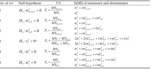
傳統綜合變方分析，對於從事栽培試驗 或育種的研究者來說，在計算上並沒有造成 太 大 的 困 難 ， 分 析 過 程 中 所 需 計 算 之 平 方 和，與其對應之均方期望值列於Table 2。 這 些 算 式 均 適 合 以 桌 上 型 或 掌 上 型 的 計算器 (desk calculator, hand calculator) 來做計算。研究者希望有個粗略的分析，於 是有可能忽略不均質的事實，直接進行傳統 的綜合變方分析。本節將說明在此情況下會 究竟會出現何種風險。以往文獻中提到的風 險 是 第 一 型 錯 誤 率 上 升(LeClerg 1962, p.231)，我們在下列兩個模擬試驗的結果， 發 現 在 某 些 效 應 的 檢 定 上 第 一 型 錯 誤 率 上 升，但是有些則下降，或者是相當穩定。對 於這些不同的反應，我門將以圖形的方式呈 現。這一節的目的在於將可能出現的風險以 實例略加說明，並且做為下一節提出合理分 析的動機。 我們根據Table 3 所列的均方期望值， 將各種形式的F檢定列於下表，我們將以模 擬研究的方式，去探討各種形式F檢定受均 方 非 均 質 性 影 響 的 情 形 。 我 們 依 據 Janky (2000) 的建議，在F檢定時，不做任何均 方合併的動作，因為將均方合併雖然增加了 分 子 或 分 母 的 自 由 度 ， 但 是 檢 定 力 提 升 有 限 ， 而 且 不 利 於 對 第 一 型 錯 誤 率 的 控 制 。 Table 4 顯示出F統計量所牽涉的變方成分 的 個 數 ， 若 是 有 兩 種 不 同 的 變 方 成 分 ， 例 如，F ，所牽涉的變方成分為₁ 2 e

σ

與

σ

_{S L V}2_{× ×} ， 我 們 直 覺 上 能 理 解 其 遭 受 非 均 質 性 的 衝 擊 程度應該會是超過{ , , }F₂ K F₆ ，因為除了F₁ 以 外 的 檢 定 所 牽 涉 的 變 方 成 份 的 個 數 超 過 2。 本 節 中 的 模 擬 試 驗 也 驗 證 了 我 們 的 直 覺 ， 就 是 在

σ

_{S L V}2_{× ×} ，

σ

_{L V}2_× ，

σ

_{S V}2_× ，

σ

_{S L}2_× ， Table 2. Formulas for computing sum of squares required by conventional combined analysis of variance.

S.O.V df SS E(MS) Season (S) s − 1 SSS 2 ... .... ˆ ( i ) rvl

∑

y −y Location (L) l−1 SSL 2 . .. .... ˆ ( j ) srv

∑

y −y S

×

L (s−1)( 1)l− SSS L× 2 .. ... . .. .... ( _{ij i j} ) vr

∑∑

y −y −y +y Rep(S

×

L) sl r( −1) SSRep v

∑∑∑

(yijk.−yij..)2

Variety(V) v−1 SSV 2 ... .... ( h ) slr

∑

y −y S

×

V (s−1)(v−1) SSSV 2 .. ... ... .... ( _{i h i h} ) lr

∑∑

y −y −y +y L

×

V ( 1)(l− v−1) SSL V× sr

∑∑

(y. .j h−y. ..j −y...h+y....)2 S

×

L

×

V (s−1)( 1)(l− v−1) SS_{S L V× ×} 2 . .. .. . . ... . .. ... .... ( ij h ij i h j h i j h ) r

∑∑∑

y −y −y −y +y +y +y −y Error sl r( −1)(v−1)

SS

_E 2 . . .. (yijkh−yijk −yij h+yij)

∑∑∑∑

Total slvr−1

SS

T 2 .... (yijkl−y )

∑∑∑∑

Table 3. Expected mean squares of conventional combined analysis of variance table. S.O.V df SS E(MS) Season (S)

s

−

1

SS

S 2 2 2 2 ( ) e

v

R S L

rv

S L

rvl

S

σ

+

σ

_×

+

σ

_×

+

σ

Location (L)

l

−

1

SS

L 2 2 2 2 ( ) e

v

R S L

rv

S L

rvs

L

σ

+

σ

_×

+

σ

_×

+

σ

S

×

L

(

s

−

1)( 1)

l

−

SS

_{S L×}

σ

_e2

+

v

σ

_{R S L}2_{( × )}

+

rv

σ

_{S L}2_× Rep(S

×

L)

sl r

(

−

1)

SS

_Rep

σ

_e2

+

v

σ

_{R S L}2_{( × )} Variety(V)

v

−

1

SS

V

σ

e2

+

r

σ

S L V2× ×

+

rl

σ

S V2×

+

rs

σ

L V2×

+

rsl

τ

V2 S

×

V

(

s

−

1)(

v

−

1)

SS

_SV

σ

_e2

+

r

σ

_{S L V}2_{× ×}

+

rl

σ

_{S V}2_× L

×

V

( 1)(

l

−

v

−

1)

SS

_{L V×}

σ

_e2

+

r

σ

_{S L V}2_{× ×}

+

rs

σ

_{L V}2_× S

×

L

×

V

(

s

−

1)( 1)(

l

−

v

−

1)

SS

_{S L V× ×}

σ

_e2

+

r

σ

_{S L V}2_{× ×} Error

sl r

(

−

1)(

v

−

1)

SS

_E

σ

_e2 Total

slvr

−

1

SS

T

Table 4. F statistics for testing various effects and variance components involved.

No. of vc‡ _{Null hypothesis T.S. E(MS) of numerator and denominator}

2 H0:

σ

S L V2× × =0 1 S L V e MS F MS × × = σe2+rσS L V2× × 2 e σ 3 H0:

σ

L V2× =0 2 L V S L V MS F MS × × × = σe2+rσS V V2× × +rsσL V2× 2 2 e r S L V σ + σ × × 3 2 0: S V 0 H

σ

× = 3 S V S L V MS F MS × × × = σe2+rσ2S L V× × +rlσS V2× 2 2 e r S L V σ + σ × × 4 2 0: V 0 H

τ

= † ₄ V SLV SV LV MS MS F MS MS + = + 2 2 2 2 2 2σe+2rσS L V× × +rlσS V× +rsσL V× +rslτV 2 2 2 2 2σe+2rσS L V× × +rlσS V× +rsσL V× 4 H0:

σ

s2=0 5 S S L MS F MS × = 2 2 2 2 ( ) e v R S L rv S L rvl S σ + σ × + σ × + σ 2 2 2 ( ) e v R S L rv S L σ + σ × + σ × 4 2 0: L 0 H

σ

= 6 L S L MS F MS × = 2 2 2 2 ( ) e v R S L rv S L rvs L σ + σ × + σ × + σ 2 2 2 ( ) e v R S L rv S L σ + σ × + σ × † 2 _{( ) /(}2 ₁₎ v Vh V v τ =

∑

− −

‡_{no. of vc : number of variance components involved in the corresponding F test.}

幾 個 變 方 成 分 只 要 其 值 明 顯 大 於 0 ， 則 2 6 { , , }F _K F 的第一型錯誤率幾乎不受非均 質性的影響。 我 們 首 先 以 模 擬 的 方 式 探 索 非 均 質 性 對於F 的衝擊。非均質性會提升第一型錯誤₁ 的機率，這個性質在 CR 設計的模式(或稱 單因子的變方分析模式)，就可以很明顯的 感覺到。我們以模擬的方式來瞭解第一型錯 誤率如何隨非均質性增加而上升。為了方便 以圖形的方式呈現非均質性的影響，我們嘗 試定義一個測度非均質程度的指標，非均質 性的程度以類似於Bartlett 的檢定統計量的

方式來度量 2 2 2 2 {log( ) log( )} log( ) log( ) i i H t σ σ σ σ = − = × −

∑

∑

這個定義可能不是很完美，但是對於將模擬 研 究 的 結 果 以 簡 潔 的 圖 形 呈 現 卻 很 有 助 益。上述的定義是來自M. S. Bartlett 的均 方均質性檢定的統計量 2 2 2 2 2 ( ) log log , ( / ) 1 {1/[3( 1)]}( (1/ 1/ )) / i i i i i i i i M v s v s s v s v C t v v M C χ = − = = + − − =

∑

∑

∑

∑

∑

∑

上

t

是指均方的個數 2_{, 1, 2, ,} i s i= _K t，v 則_i 是 代 表 各 均 方 的 自 由 度 。 我 們 定 式 之 義 的

H

指標，是將變方值

σ

_i2取代均方值s_i2，並 且省略自由度

v

_i，主要的原因是由於綜合變 方是均衡的設計，在同樣的設計下比較異質 性應該是不需要考慮重複數或是自由度。模 擬所根據的模式是

1, 2, , ;

1, 2, ,

ij i ij

y

i

a

j

n

µ τ ε

= + +

=

_K

=

_K

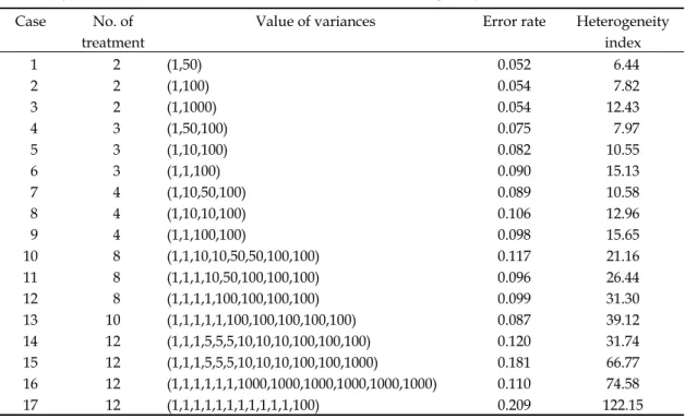
為了檢測第一型錯誤之機率，令τi= ∀0, i。 Table 5 中之數字為第一型錯誤的機率。 Table 5 顯示第一型錯誤機率大致上隨 著異質性程度增加而上升，Fig. 1 顯示其上 升之趨勢。當最小的變方與最大變方的比值 為 1000 倍時(case 17)， 第一型錯誤機率 有可能高達0.21 而不是所宣稱的 0.05。 以 上 雖 然 考 慮 的 是 簡 單 的 單 向 變 方 分 析模式或是CR 設計的模式，但是其結果與 典 型 綜 合 分 析 的

F

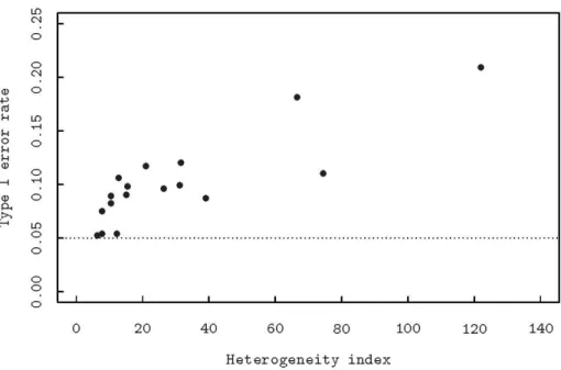
₁檢 定 應 該 類 似 。 在 探討 複雜的「典型」的綜合變方分析之前，我們 先看看最簡單的綜合變方分析模式，此模式 只 包 含 地 區( 或 稱 環 境 ) 與 品 種 兩 因 子 ，

Table 5. Type I error rate of F statistic under various cases of heterogeneity of error variances. Case No. of

treatment

Value of variances Error rate Heterogeneity index 1 2 (1,50) 0.052 6.44 2 2 (1,100) 0.054 7.82 3 2 (1,1000) 0.054 12.43 4 3 (1,50,100) 0.075 7.97 5 3 (1,10,100) 0.082 10.55 6 3 (1,1,100) 0.090 15.13 7 4 (1,10,50,100) 0.089 10.58 8 4 (1,10,10,100) 0.106 12.96 9 4 (1,1,100,100) 0.098 15.65 10 8 (1,1,10,10,50,50,100,100) 0.117 21.16 11 8 (1,1,1,10,50,100,100,100) 0.096 26.44 12 8 (1,1,1,1,100,100,100,100) 0.099 31.30 13 10 (1,1,1,1,1,100,100,100,100,100) 0.087 39.12 14 12 (1,1,1,5,5,5,10,10,10,100,100,100) 0.120 31.74 15 12 (1,1,1,5,5,5,10,10,10,100,100,1000) 0.181 66.77 16 12 (1,1,1,1,1,1,1000,1000,1000,1000,1000,1000) 0.110 74.58 17 12 (1,1,1,1,1,1,1,1,1,1,1,100) 0.209 122.15

Fig. 1. Simulated type I error rate versus heterogeneity index . The error rate inflates as the degree of heterogeneity is getting higher.

( ) ( ) 1, 2, , ; 1, 2, , ; 1, 2, , ijk i j i k ik ijk y L R V LV i l j r k v

µ

ε

= + + + + + = _K = _K = _K 在機差變方均質的情況下，變方分析表中各 均方之期望值如 Table 6 所示。 我們考慮下列兩個檢定統計量 1 , 2 L V V E L V MS MS F F MS MS × × = = 前 者 是 檢 定 H0:

σ

L V2× =0， 後 者 是 檢 定 2 0: vk k 0 H ∑ V = 。在此兩假說均成立下， 以 模 擬 的 方 式 求 得 各 種 異 質 程 度 下 的 第 一 型 誤差率，並以 Fig. 2 的方式呈現，實心點與 空心點分別為為

F

₁與

F

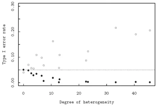
₂的第一型錯誤率。 兩 者 在 非 均 質 程 度 增 大 時 呈 現 相 反 的 趨 勢，前者呈上升之趨勢，後者則出現下降的 趨勢，可見變方異質性對第一型錯誤率的衝 擊有一種以上的方式，並不只是像一般認為 僅是讓第一型錯誤率膨脹而已。 最後呈現的的是典型的綜合變方分析模 式下的第一型錯誤率的圖，Fig. 3 呈現的趨勢 與Fig. 2 類似，但是在異質性指數值比 0 稍 大一些，第一型錯誤率就開始上升或下降的 趨勢，這反應出異質性指數似乎是需要加入 自由度

v

_i才能做Fig. 2 與 Fig. 3 之比較。傳 統綜合變方分析雖有上述的缺點，但是對

F

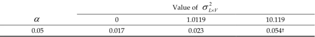
₂ 而言當

σ

_{L V}2_× 的值大到某一程度時，其第一型 錯誤率仍能維持相當穩健的程度，如Table 7 所示。 Table 7 顯示三種不同的

σ

L V2× 值下，以模 擬方式求得的第一型錯誤率。在

σ

_{L V}2_× 趨近於 0 時，機差變方的異質性會造成比較保守的

F

檢定，但是隨著

σ

_{L V}2_× 的值增大，第一型錯 誤率也趨近名目值0.05 (nomial value)。 由 於 本 文 主 要 是 介 紹 一 種 能 在 變 方 異 質性下可以合理分析的方法，並無意通盤檢 討 傳 統 綜 合 變 方 分 析 的 在 變 方 異 質 性 下 的 種種可能性質，因此我們對傳統綜合變方分 析的討論在此告一段落，並往前進入本文的 核心部份。

Table 6. Expected mean squares derived from the combined analysis of variance model having only location and variety factors.

S.O.V df SS E(MS) Location (L)

l

−

1

MSL

σ

e2+v

σ

r l2( )+rv

σ

L2 Rep (R)

l r

(

−

1)

MSRep

σ

e2+v

σ

r l2( ) Variety (V)

v

−

1

MSV 2 2 2 e r L V rl V

σ

+

σ

× +

τ

L V

×

( 1)(

l

−

v

−

1)

MS

_{L V×} 2 2 e r L V

σ

+

σ

_× Error

l r

(

−

1)(

v

−

1)

MS

_E

σ

e2 Total

lvr

−

1

Table 7. Empirical type I error rate for testing 2 0: k 0

H

∑

V = of conventional ANOVA under three different values of

σ

_{L V}2_× . Estimated

α

ˆ

is obtained from a simulation study using parameters defined in Table 15.

Value of

σ

_{L V}2_×

α

0 1.0119 10.119

0.05 0.017 0.023 0.054†

†_{Estimate of error rate obtained from 2000 simulation runs.}

Fig. 2. Simulated type I error rate versus heterogeneity index. The open circle ○ indicates the error rate of the F test of Variety by Location interaction. The solid circle ● shows the error rate of F test of Variety effect. Both the interaction effects and variety effects are assumed

null, namely,

σ

_{V L}2_×

=

0

and

∑

Vk2=0. Interestingly, error rate of these two F tests have

Fig. 3. Simulated type I error rate versus heterogeneity index. The model used in simulation is referred as ‘typical combined analysis of variance model’ which is more complicated than the one in Figure 2. Similarly as in Figure 2, open circle ○ goes up and solid circle ● goes down as the degree of heterogeneity increases.

以混合模式的觀點看綜合變方分析模式

在 看 過 上 一 節 中 第 一 型 錯 誤 率 上 升 與 下降的情況後，在這一節中希望能藉由近代 線型混合模式的理論，找出一個可能的解決 方法。往下將先說明，近代線型混合模式在 理 論 上 已 經 將 傳 統 上 的 嚴 苛 前 提—機差變 方需具均質性—放寬，使其較符合實際資料 所呈現的現象；然後說明現有的統計軟體如 何 在 放 寬 前 提 下 計 算 出 實 用 者 (practitioner) 所要的統計分析。在正式說 明之前，我們將傳統變方分析的模式以矩陣 的表示法陳列於下: = + + Y Xβ Zb ε 式 中 之

β

為 固 定 型 效 應 ， 例 如 在 本 文 中 之 品種效應；

b

為隨機型效應，例如本文中提 到的季節，年份，地區等效應；

ε

則為機差。 傳 統 綜 合 變 方 分 析 模 式 的 前 提 是 變 方 的 均 質性，以矩陣的符號表示則為 2

~ (0,

N

σ

e

)

ε

I

以另外一個方式來說明就是，

Y

的變方矩 陣可以表示成 2 Var( )Y =ZGZ'+

σ

eI 上式中之隨機型效應的變方以符號

G

表 示，即 G=Var( )b 。本文前面的部份提及， 這個模式難以符合現實的情形，因為機差均 方 通 常 呈 現 異 質 性 。 近 代 線 型 混 合 模 式 (linear mixed models) 的理論，已經可以

做到放寬變方均質性的前提，也就是說分析 下列變方結構

Var( )Y =ZGZ' R+

的理論架構已經成熟，也有現成的統計套裝 軟體可供計算，例如 SAS 的 proc mixed。 我 們 往 下 將 以 兩 個 數 例 來 說 明 如 何 利 用 SAS 的 proc mixed 來 計算。有關 SAS proc mixed 的 細 節 請 參 考 SAS/STAT (1996) 手冊。 在進入實際數例之前，我們以一個假設 的資料形式來說明機差的變方結構。假設地 區數為 4，重複數為 3，品種數為 2，則資 料的總觀測值個數是24 (=

4 3 2

× ×

)。一般 試驗者會將資料整理成Table 8 的形式，亦 即 以 地 區 為 群 集(cluster)， 總 共 有 四 個 群 集，每個群集裡有 6 個觀測值。為了讓讀者 清 楚 的 瞭 解 資 料 的 排 列 方 式 與 混 合 模 式 的 應 用 有 關 ， 我 們 除 了 上 述 的 符 號

y

_{l r v, ,} 以 外，另外也用數字來幫助說明。Table 9 中 的數字是從隨機數字表裡抽出的 24 組兩位 數字，純粹為了方便說明在統計分析的過程 中 ， 資 料 的 排 列 方 式 。 隨 機 數 字 是 摘 自 於 Snedecor and Cochran (1988, p.460)。我們 比較習慣的思考方式是將三個下標

{ , , }

l r v

讓最右邊的

v

變動最快，最左邊的

l

則變動 最慢，因此我們思考的觀測值向量的形式為 111 112 121 122 131 132 211 212 221 222 231 232 311 312 321 322 331 332 411 412 421 422 431 432 ( , , , , , , , , , , , , , , , , , , , , , , , ) ' y y y y y y y y y y y y y y y y y y y y y y y y = y 根據上述的排列方式，我們不難識別出每個 地區的 6 個觀測值為一群集，以第一個下標

l

為 群 集 的 代 號 ， 例 如

y

₁₁₁，

y

₁₁₂，

y

₁₂₁， 122

y

，

y

₁₃₁，

y

₁₃₂，一共有四個群集。也就 是說，觀測值的排列方式是前 6 個觀測值屬 於第一個地區，其次6 個觀測值屬於第二個 地區，再其次的 6 個觀測值屬於第三個地 區，最後的 6 個地區則屬於第四個地區。用 實際數字表示如下 ( 54, 90, 46, 57, 32, 06, 26, 39, 62, 79, 65, 36, 36, 56, 56, 98, 73, 31, 82, 47, 29, 05, 08, 80 ) ' = y 為了配合說明 proc mixed 的敘述， 我們調整下標的排列秩序為

y

_rvl，讓

l

為 變動最快的下標，

r

為變動最慢的下標 111 112 113 114 121 122 123 124 211 212 213 214 221 222 223 224 311 312 313, 314 321 322 323 324 ( , , , , , , , , , , , , , , , , , , , , , , ) ' y y y y y y y y y y y y y y y y y y y y y y y y = y 上 式 中 之 群 集 是 由

{ , }

r v

兩 者 的 組 合 構 成，共有6 個組和， (11,12, 21, 22,31,32) ， 每 一 橫 排 為 一 群 集 ， 例 如

y

111，

y

112， 113

y

，

y

114。 下 列 的 數 字 表 示 是 輔 助 上 面 的 符 號 說 明， ( 54, 26, 36, 82, 46, 62, 56, 29, 32, 65, 73, 08, 90, 39, 56, 47, 57, 79, 98, 05, 06, 36, 31, 80 ) ' = y 例 如 對 於 第 一 群 集 的 四 個 數 字(54, 26, 36, 82)，參看 Table 9 中數字所在的位置，以明 瞭群集形成的方式。在使用 proc mixed 時, 必須清楚的瞭解群集(cluster)為何。

Table 8. Notations for individual observations. The subscripts

{ , , }

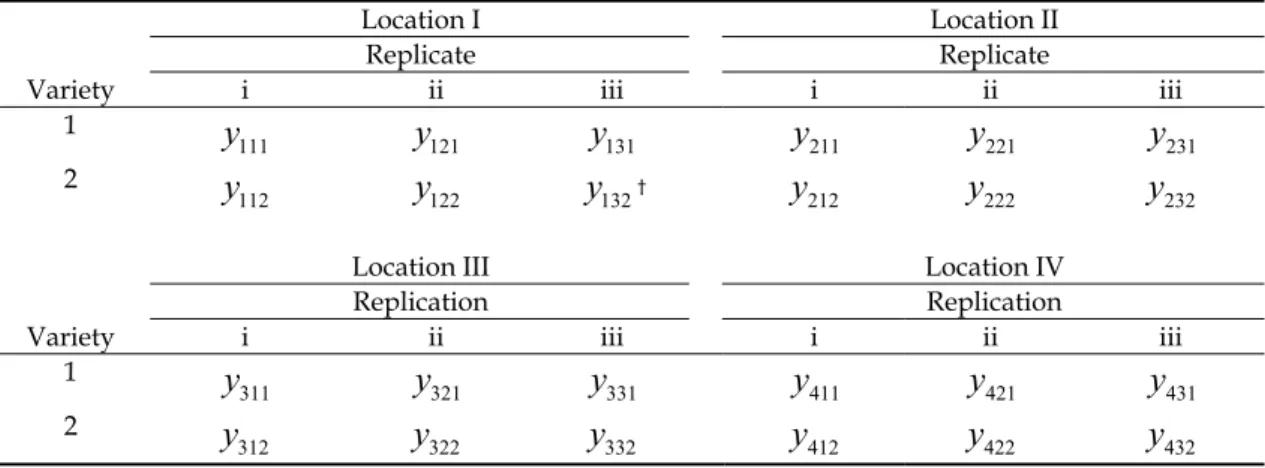
l r v

in

y

_lrv denotes the lth location, rth replicate and vth variety, respectively.

Location I Location II

Replicate Replicate

Variety i ii iii i ii iii

1 111

y

y

₁₂₁

y

₁₃₁

y

₂₁₁

y

₂₂₁

y

₂₃₁ 2 112

y

y

₁₂₂

y

₁₃₂† 212

y

y

₂₂₂

y

₂₃₂

Location III Location IV

Replication Replication

Variety i ii iii i ii iii

1 311

y

y

₃₂₁

y

₃₃₁

y

₄₁₁

y

₄₂₁

y

₄₃₁ 2 312

y

y

₃₂₂

y

₃₃₂

y

₄₁₂

y

₄₂₂

y

₄₃₂ †

Notation y132 denotes that the tomato yield observation collected from location 1 replicate 3 and

variety2.

Table 9. Hypothetical data corresponding to the previous table. The numbers in this data are used For illustrating the rearrangement of observations. The rearrangement of observations into clusters is essential before employing statistical software to do mixed model analysis and will be discussed subsequently.

Location I Location II

Replicate Replicate

Variety i ii iii i ii iii

1 54 46 32 26 62 65

2 90 57 06† _{39 79 36}

Location III Location IV

Replication Replication

Variety i ii iii i ii iii

1 36 56 73 82 29 08 2 56 98 31 47 05 80 現 以 第 一 群 集(54,90,36,56)機 差 的 變 方 結構為例，說明其可能的結構，第一種可能 的結構其表示方式為 2 1 2 2 2 3 2 4 0 0 0 0 0 0 Var( ) 0 0 0 0 0 0 σ σ σ σ       =_{ }     11 ε 上式中之ε11=(ε ε₁₁₁, ₁₁₂,ε ε₁₁₃, ₁₁₄)，這是對應於 111 112, 113 114 (y ,y y ,y )也就是(54, 90, 36, 56)的機 差 。SAS proc mixed 的 處 理 方 式 是 令

Var(ε11)=K=Var(ε32)，也就是令此6 個群集 有相同的機差變方結構。此種變方結構顯示 每一個地區之機差都不相等。下一種可能的 結 構 是 將 四 個 機 差 變 方 歸 類 成 兩 層 (strata)，地區一與地區二歸為一層，地區 三與地區四歸為另一層，表示方式如下 2 1 2 1 2 2 2 2 0 0 0 0 0 0 Var( ) 0 0 0 0 0 0 σ σ σ σ       =_{ }     11 ε

當然也有可能是 2 2 2 2 1 1 1 2 diag{ ,σ σ σ σ ，或, , } 歸類成三層的情形 2 2 2 2 1 2 2 3 diag{ ,σ σ σ σ ，所以, , } 可 能 的 情 形 個 數 隨 著 地 區 數 的 增 加 而 大 幅 增加。究竟要如何判斷何種結構才是適合的 結構? 我們建議的策略是先求出各地區之機差 均方

s

_l2,l=1, 2,3, 4，以此處的假設資料為例 就是做四個單獨的RCRD 變方分析即可取得 2 l

s

值。而後以

s

_l2值的相對大小分成幾層，也 就是將數值接近者分類成同一層，數值差異 較 大 者 分 至 不 同 層 。 先 猜 測 幾 種 適 合 的 分 層，而後根據AIC 或 BIC 的值來判斷先前猜 測 的 何 者 較 適 合 ，AIC 與 BIC 是 所 謂 的 information criterion，是根據對數概度函數 值修正後的值，數值越小者越有可能接近真 正的變方結構。這個猜測的共變方結構與真 正的結構可能會不一樣，在統計上稱之為工 作變方結構(working covariance structure)。

我 們 認 為 以 上 的 構 想 是 有 相 當 的 應 用 價值，藉由資料的重新排列，配合現有的統 計軟體，以達到分析區域產量試驗資料的目 的。用混合模式來描述時間上或空間上有關 聯 的 資 料 ， 常 見 於 討 論 混 合 模 式 應 用 的 文 獻，例如， Littell et al. (1996) 與 Pinheiro and Bates (2000)。在此等文獻中提到的群 集 多 為 直 覺 上 容 易 明 白 的 ， 例 如 同 一 個 個 體，例如一位病人，在不同時間點的觀測值 構成一個群集，或是一區集內的數個試區構 成一個群集，因為兩個相鄰的試區作物產量 相關較高，距離較遠的兩個試區作物產量的 相關較低，因此同一個區集中的數個試區產 量視為一個群集。但是在本文中將區集與品 種的組合視為群集，在直覺上是不具任何意 義的，只是為了配合現有的理論與計算軟體 而形成的觀念。也可能是因為缺乏直覺的意 義，所以此類資料沒有被Littell et al. (1996) 與 Pinheiro and Bates (2000) 收 錄 及 討

論 ， 這 也 是 本 文 作 者 認 為 值 得 介 紹 的 新 觀 念。在下一節中我們以兩組實際資料的分析 說明整個分析過程。

蕃茄區域產量試驗資料之分析

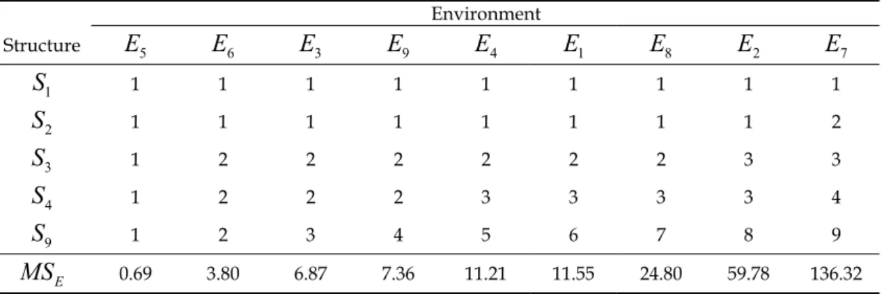
第 一 個 要 分 析 的 數 據 是 之 前 提 到 的 蕃 茄資料，本資料列於Appendix 3。本資料 為 9 個環境下的 RCBD 資料，經由初步的 9 個獨立的變方分析，求出機差均方並按其大 小順序排列於 Table 9。Table 9 中之共變方 結 構

S S S S

₁

, , ,

_{2 3 4}與

S

₉分 別 將 機 差 變 方 劃 分 成 1,2,3,4,9 層 ， 我 們 將 各 結 構 對 應 的 AIC 與 BIC 值列於 Table 11。表中之 AIC

與 BIC 值顯示

S

₄在五個可能的共變方結構 中是最佳的。其AIC 值(681.2)與

S

₉(680.7) 幾乎相等，以 BIC 的觀點來看

S

₄(692.3 < 699.7) 較優。 用 來 執 行 分 析 的 SAS 程 式 列 於 Appendix 1，此程式由兩部份構成，第一 部份是資料輸入及機差變方分層，第二個部 份是核心的部份，以 proc mixed 做混合 模式的計算。現在我們摘錄第二部份如下並 做說明

proc mixed data = d00 ; class env var rep s4 ;

model yield = var / ddfm = satterth solution ; random rep(env) env env * var ;

repeated rep * var / type = vc subject = env group = s4 ; lsmeans var / dif ;

run ; 程式中之 env，var，rep，yield 與 s4 分 別代表 環境，品種，重複，蕃茄產量與第四 種分層結構(見 Table 10)。上述程式只做一種 分層劃分s4，假如要做分層劃分 s3，只要將 class 敘述與 repeated 敘述兩者的 s4 改 成 s3 即可。第二部份的最關鍵的敘述是 repeated 敘述，其功能是用來指定機差變方 的 形 式 ， r e p * v a r 的 用 意 是 要 建

Table 10. Identification number of stratum of each possible variance structure. Five possible variance structure and the error mean squares are listed below.

Environment Structure

E

₅

E

₆

E

₃

E

₉

E

₄

E

₁

E

₈

E

₂

E

₇ 1

S

1 1 1 1 1 1 1 1 1 2

S

1 1 1 1 1 1 1 1 2 3

S

1 2 2 2 2 2 2 3 3 4

S

1 2 2 2 3 3 3 3 4 9

S

1 2 3 4 5 6 7 8 9 E

MS

0.69 3.80 6.87 7.36 11.21 11.55 24.80 59.78 136.32 †

Structure

S

₃ has 3 strata and environment

E

₆ belongs to stratum no. 2. Table 11. Information criteria for determination of covariance structure.

Information Stratum structure

criterion

S

₁

S

₂

S

₃

S

₄

S

₉ AIC 730.9 702.0 692.0 681.2 680.7 BIC 737.2 709.9 701.6 692.3 699.7 Reduction in AIC - 28.9† _{10.0 10.8 0.5} difference in df - 1 1 1 5 †

Reduction in AIC value 28.9 = 730.9 – 702.0 > 3.841. This amount of reduction shows that Structure S2

is better than Structure S1.

構我們所需要的群集，也就是將觀測值排列 的 順 序 調 整 為

Y

_rvl ， 每 一 群 集 由 9 (l=1, 2, ,9K )個環境構成，subject = env 是 說 明 群 集 中 的 個 體 即 為 「 環 境 」， 一 共 12 (rep*var) 共有 12 個組合) 個群集。因此， 整 個 資 料

y

的 機 差 成 分

ε

其 變 方 矩 陣 為 區 塊對角矩陣(block diagonal matrix)，由 12 個相同的區塊B=Var( )εrv 構成，其結構如下: Var( ) Var( ) Var( ) Var( ) Var( )         =         0 0 0 0 0 0 ε 0 0 0 0 0 0 L L M M O M M L L 11 12 42 43 ε ε ε ε 每個區塊B 的結構則由 type 及 group 兩個選項(option)來註明，type = vc 目的 在於讓 B 矩陣具有對角矩陣的結構，對角 線 上 的 元 素 由 9 個 變 方 成 分 (vc) 構 成 ， group = s4 則將此 9 個變方成分歸類成四 層，也就是下列的形式 2 2 2 2 2 2 2 2 2 3 3 2 3 1 2 4 3 2 Var( ) diag{ , , , , , , , , } 1, 2,3, 4; 1, 2,3 r v σ σ σ σ σ σ σ σ σ = = = = rv B ε 上 式 中 之 四 個 變 方 成 分 ， 2 2 2 2 1 2 3 4 σ <σ <σ <σ 分別對應於四個分層。我們不難感覺到這個 區 塊 矩 陣 比 起 傳 統 上 均 質 的 機 差 變 方 矩 陣 2 e σ I 會更接近資料的本質。第二個數例是 LeClerg 書上的例子，是大麥的區域產量試 驗資料，為了方便參考， 我們將此資料列

於 Appendix 4。這個例子的均方均質性前 提是滿足的，可以合理的執行傳統的綜合變 方分析，但是我們仍將其做為說明的例子。 在這個數例，含有年份，地區與品種三個因 子，分別以 year，loc 與 var 表示；年份， 地區與品種的變級數各為 2，4 與 5；重複 數則為 3。如前例所述，以重複與品種的組 合構成 15 (=3×5) 個群集，每個群集包含 8 (=2×4，年份與地區的組合數) subject。 在此情況下，每個群集中有8 個機差變方， 對於分層的方式，我們僅考慮三種種分層的 方式，一是分成8 層，另一是分成 1 層，介 於這兩極端的則是分成兩層。我們做這樣考 慮 的 原 因 是 觀 察 過 各 單 獨 試 驗 的 機 差 均 方，見 Table 13，而後做的決定。換句話說， 我們究竟是需要 8 個變方成分參數來描述 群集的變方結構 2 2 2 2 2 2 2 2 11 12 13 14 21 22 23 24 diag{σ σ σ σ σ σ σ σ, , , , , , , } = B 或是只要 1 個變方成分參數 2 8 e

σ

=

×

B

I

或是兩個變方成分的參數 2 2 2 2 2 2 2 2 2 2 1 1 1 1 1 1 2 2 1 2 diag(σ σ σ σ σ σ σ σ σ σ, , , , , , , , , ) = B 用 來 計 算 的 SAS 程 式 求 列 於 Appendix 2，計算所得的對數概度函數值及 AIC，BIC 值列於 Table 14。上述程式中的 repeated 敘述大致上與前一個數例相似，由於這個綜 合試驗是由 8 (

= × = ×

s l

2 4

) 個環境下的 產 量 試 驗 所 構 成 的 ， 因 此 type=vc 與 subject=year*loc 是說明這 8 個試驗各自 的 機 差 變 方 成 分 可 能 不 同 ， 另 外 group=s2 是用來指定這 8 個試驗機差可 歸類成兩層。AIC 值顯示：機差結構

S

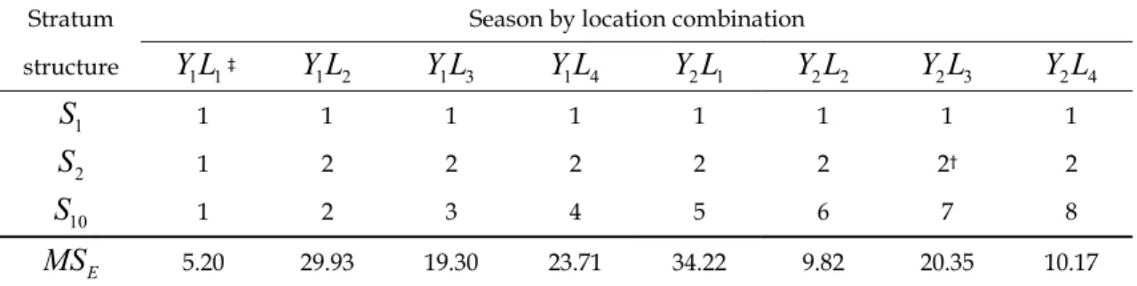
₁是 三者中最好的，因為其AIC 值 829.2 最小， 將機差結構分成兩層S₂或是10 層S10均不如 單一的一層。換句話說機差均質性的假說是 成立的，因此我們可以用傳統的綜合變方分 析法來進行分析。

新的方法與傳統變方分析的比較

我 們 以 模 擬 研 究 (simulation study) 的方式，比較新方法與傳統變方分析，看看 新 的 方 法 對 於 第 一 型 錯 誤 率 的 控 制 是 否 有 改善。我們只考慮了一個情形，就是蕃茄區 域試驗資料，將 9 個不同的機差變方成分 歸類成四層來描述其機差變方結構。模擬研 究的過程敘述如下: 1) 設定參數的數值如 Table 15。 為 了 使 參 數 的 數 值 不 會 大 幅 偏 離 實 際 上 的 栽 培 或 育 種 資 料 ， 我 們 先 以 附 Appendix 1 的程式分析蕃茄的資料，將 機差分成9 層(s9)，而後將所求出之變方 成 分 的 估 值 設 為 參 數 值 ， 但 是 品 種 效 應 訂為 0，交感效應也訂為 0。 2) 將 9 個機差變方分為四層如 Table 11 的 4

S

所示。 3) 按照 1) 所設定的參數值產生隨機樣本, 每個樣本含有 108 個觀測值。 4) 利 用 proc mixed 計 算 檢 定 0

:

k

0

H V

=

的 F 統計量，並判定是否拒 絕虛無假說。 5) 重複執行步驟 3) 與 4)，將 1000 個樣 本 F 值 被 拒 絕 的 比 率 求 出 即 為 模 擬 所 得的第一型錯誤率。 在此必須說明的是在模擬研究時，我們 是將 9 個機差的變方依其假設的參數值分 成四層，而不是根據每次估計所得的 9 個 機差均方值去分層，主要原因是在程式的撰 寫上困難度太高無法做到。 模 擬 得 到 的 第 一 型 錯 誤 率 列 於 Table 16，表中之 New method 顯示出對於品種 差 異 之 檢 定

H V

₀

:

_k

=

0,

k

=

1, 2,3

， 在

2

₀

L V

σ

×

=

時，其第一型錯誤率 0.066 較符合 名 目 值 0.05，傳統的方法所得的錯誤率為 0.025 有明顯低估的情形，一如 Fig. 2 與 Fig. 3 中 之 實 心 點 所 示 ； 但 是 在 2 _1.012 L V σ × = 時，新方法的第一型錯誤率明顯不如傳統的 方法，可能的原因在於傳統的方法所用的檢 定統計量 F=MSV/MSL V× 沒有牽涉到變方 成分

σ

_{L V}2_× 的估算，而混合模式中是以受 限 最 大 概 度 法 估 算 此 成 分 ， 通 常 由 於 2 ₀ L V σ × ≥ 的限制，使致 σˆL V2× 有正向偏差的 現 象 (bias upward) 。 這 種 偏 性 在 2 ˆL V 10.119 σ × = 時程度減弱，使得第一型錯誤 率逐漸向名目值靠近。

Table 12. Results of statistical analysis of tomato data. Nine environments

MS

_E are categorized into 4 strata and the associated mixed effects model is employed accordingly.

(1) Estimates of variance components of random effects

2 2 2

ˆ

_rep

2.97,

ˆ

_env

413.15,

ˆ

_{env var}

10.12

σ

=

σ

=

σ

_×

=

(2) Estimates of error variances

2 2 2

1 2 3

ˆ

0.72,

ˆ

5.55,

ˆ

25.44

σ

=

σ

=

σ

=

(3) Testing variety effects

0 1 2 3 1 2

:

0

5.16,

2,

14.4,

value=0.0204

H v

v

v

F

v

v

p

=

=

=

=

=

=

−

Table 13. Values of error mean square obtained from each individual experiment and three possible covariance structure of these error mean squares.

Stratum Season by location combination structure

Y L

_{1 1}‡ 1 2

Y L

Y L

_{1 3}

Y L

_{1 4}

Y L

_{2 1}

Y L

_{2 2}

Y L

_{2 3}

Y L

_{2 4} 1

S

1 1 1 1 1 1 1 1 2

S

1 2 2 2 2 2 2† ₂ 10

S

1 2 3 4 5 6 7 8 E

MS

5.20 29.93 19.30 23.71 34.22 9.82 20.35 10.17

†_{The error mean square of} Y L_{2 3 is categorized into stratum number 2.}

‡_{This notation indicates that a barley yield trial was conducted in year Y1 and on location} L_1.

Table 14. Information criteria for determining error variance structure.

Information Covariance structure

criterion

S

₁

S

₂

S

₈

2

− ×

log-likehood 819.2 816.6 809.1 AIC 829.2 830.6 833.1 BIC 822.7 822.8 817.5 Reduction in AIC - 1.4 2.5 difference in df - 1 6

Table 15. Hypothetical parameter values used in the simulation study. These parameter values are actually estimates obtained from the tomato regional yield data.

Effect Value Variety (V)

V

_k

=

0

, for all k

Environment (L)

σ

_L2

=

411.06

Replicate (environment)

σ

_{R L}2_{( )}

=

2.5374

L V

×

2

_10.1190

L V

σ

_×

=

† 2

1.012

L V

σ

_×

=

† 2

0

L V

σ

_×

=

† Error 2 2 2 1 2 3 2 2 2 4 5 6 2 2 2 7 8 9

9.8457

54.5614

6.0733

8.8780

0.7342

3.7247

134.98

30.5618

6.8454

σ

σ

σ

σ

σ

σ

σ

σ

σ

=

=

=

=

=

=

=

=

=

†_{Three different} 2 L V

σ

_× were used in the simulation study.

Table 16. Simulated type I error rates of both conventional method and the proposed method. Entries are based on 3,000 simulated runs.

Value of

σ

_{L V}2_×

Method 10.119 1.012 0

Conventional 0.0457 0.0317 0.0247 New method 0.0770 0.1183 0.0527

Table 17. Number of convergence runs under 4 and 9 strata, respectively. The entries are estimates based on the results of 1,000 simulation runs.

Full model 4 strata 9 strata Reduced model

C

_f † f

NC

C

_f

NC

_f r

C

† ₉₉₈‡ _{0 958 22} r

NC

2 0 5 15

† _{The subscripts f and r represent ‘full model’ and ‘reduced model’, respectively. The abbreviations C and}

NC denote the status ‘convergence’ and ‘non-convergence’, respectively.

‡ _{In 1,000 data sets generated, 998 of them are successfully fitted by both full and reduced models with}

error variance structure having 4 strata.

最 後 要 提 的是 有 關 於 檢定 2 0: L V 0 H σ × = 的第一型誤差控制，這是傳統方法在變方異 質性時最嚴重的問題。模擬研究的方式仍然 依循上述步驟，只是步驟 4) 的 F 檢定改為 對數概度比檢定 ( ) 2 log 2 log ( ) R r R f L M L M     − Λ = − _{ }     式中之

L

_R為受限最大概度函數 (restricted maximum likelihood)，

M

r與

M

f 分別 為 下 列 簡 化 模 式(reduced model) 與 全模

式 (full model)的代號， ( ) ( ) : : ( ) r ijk i j i k ijk f ijk i j i k ik ijk M y L R V M y L R V LV µ ε µ ε = + + + + = + + + + + 按照上述模擬的方式，執行 1000 次的模擬 結果求得的第一型錯誤率為0.031 與名目值 0.05 較接近，比起傳統綜合變方分析的第一 型錯誤率為 0.133，新的方法大幅改善了第 一 型 錯 誤 率 膨 脹 的 問 題 。 若 改 用 最 大 層 數 9

S

來描述機差變方結構，在層數為 9 時， 模 擬 的 方 式 求 得 的 第 一 型 錯 誤 率 為 0.033，此結果與層數為 4 時非常相近。

討論

在 這 節 中 我 們 說 明 與 機 差 變 方 分 類 的 層數有關的問題。前一節中我們依據 AIC 來判定層數的多少，這種決定實際上用來操 作 的 共 變 方 結 構---簡稱為「實作共變方結 構」(working variance structure)—的程序

是 proc mixed 所提出的。但是用直覺上 最 大 的 層 數 不 是 更 接 近 資 料 的 真 實 情 況 嗎？例如，在模擬研究中，一共有 9 個環 境，我們設定了 9 個不同的環境機差變方參 數值，按照最接近資料性質的分析方式應該 是將機差變方結構矩陣設定成 2 2 2 2 2 2 2 2 2 1 2 3 4 5 6 7 8 9 Var( ) diag( ,εrv = σ σ σ σ σ σ σ σ σ, , , , , , , ) 此 時 的 層 數 為 最 大 的 可 能 層 數 。 原 則 上，我們同意這是最接近資料性質的變方結 構，但是隨著環境的個數增加，變方的參數 也隨著增加，這意味著計算的負擔也增加， 而 且 遞 迴 求 算 估 值 的 演 算 法 收 斂 的 機 率 也 跟著降低。例如在這個模擬研究的例子，層 數訂為 9 時，模擬 1000 組資料，無法收 斂的次數為20 ~ 37 次，層數訂為 4 時，無 法 收 斂 的 次 數 為 0 ~ 2，此結果顯示於表 17。由此可見，除了以 AIC 值來判斷外， 在計算的觀點來看層數也不宜過多。

引用文獻

Janky DG (2000) Sometimes pooling for analysis of variance hypothesis test: A review and study of a split-plot model. Amer. Statistic. 54: 269-279.

Littell RC, GA Milliken, WW Stroup, RD Wolfinger (1996) SAS System for Mixed Models. SAS Institute. Cary, NC.

Petersen RG (1994) Agricultural Field Experiments. Marcel Dekker, New York. 409pp.

Pinheiro JC, DM Bates (2000) Mixed-Effects Models in S and S-PLUS. Springer, Berlin. 528pp. SAS Institute (1996) SAS/STAT user's guide. SAS

Appendix 1. SAS program for analyzing the tomato data using a mixed effects model. This program shows how to create a stratum variable and put it work.

* part i data input and strata formation;

* s2: two strata, s3: three strata, s4: four strata; * s1: one stratum, s9: nine strata;

data d00;

infile 'c:\tomato_env_var.dat' firstobs=2 expandtabs; input env var rep yield;

s1 = 1;

if env = 7 then do; s2 = 2; end; else do;

s2 = 1; end; if env = 7 then do; s3 = 3; end;

else if env = 5 then do; s3 = 1; end;

else do; s3 = 2; end; if env = 7 then do; s4 = 4; end;

else if env = 1 | env = 2 | env = 4 | env = 8 then do; s4 = 3; end;

else if env = 3 | env = 6 | env = 9 then do; s4 = 2; end; else do; s4 = 1; end; s9 = env; run; * part ii;

* only the case of 4 strata is computed;

* other cases can be computed by replacing s4 by s1, s2, or s9; proc mixed data=d00;

class env var rep s4;

model yield = var / ddfm=satterth htype=3 solution; random rep(env) env env*var;

repeated rep*var / type=vc subject=env group=s4; run;

Appendix 2. SAS program for analyzing barley regional yield trial data by using a mixed effects model. This program shows how to create a stratum variable and incorporate this variable in computation.

* part i data input and strata formation; * s1: one stratum, s2: two strata;

* sea: season (year), loc: location, var: variety, rep: replicate; * obs: observation no.;

data d00;

infile 'c:\experiment.dat' firstobs=2 expandtabs; input obs yield sea var loc rep;

s1 = 1; s2 = 1;

if (yr = 2 and env = 2) | (yr = 2 and env = 3) | (yr = 2 and env = 5) then do; s2=2; end;

run;

* part ii;

* only the case of two strata is computed;

* s2 can be replaced by s1 if one stratum is desired;

proc mixed data=d00;

class sea loc var rep s2;

model yield = var / ddfm=satterth htype=3 solution; random sea loc sea*loc sea*var loc*var sea*loc*var; repeated rep*var / type=vc subject=sea*loc group=s2; run;

* part iii;

* the case of 10 strata is computed;

proc mixed data=d00;

class sea loc var rep s2;

model yield = var / ddfm=satterth htype=3 solution; random sea loc sea*loc sea*var loc*var sea*loc*var; repeated rep*var / type=vc subject=sea*loc group=sea*loc; run;

Appendix 3. Tomato yield data collected by Su-Sze Yang during the years 2001 and 2002.

Replication

Year Season Location Variety 1 2 3 4 2001 1 1 1 33.40 39.20 36.67 39.20 3 35.87 34.60 30.33 39.73 4 37.93 38.27 41.40 36.13 2 1 1 84.20 77.07 82.20 89.40 3 101.07 77.07 78.07 83.40 4 81.87 89.40 74.60 85.07 2 1 44.42 43.04 36.53 36.22 3 44.75 46.96 43.81 43.91 4 37.74 38.03 39.01 39.29 3 1 33.20 30.60 29.70 33.70 3 37.20 32.40 30.50 38.30 4 25.60 29.30 32.10 27.00 2002 1 2 1 19.78 17.84 19.00 23.38 3 21.93 18.52 18.38 24.77 4 20.04 18.28 16.47 22.40 3 1 25.60 23.80 27.10 20.30 3 26.20 23.50 25.30 24.20 4 23.40 26.50 24.20 19.50 2 1 1 80.73 69.47 47.80 77.67 3 77.53 61.07 63.93 75.60 4 81.53 72.00 67.73 48.53 2 1 53.32 43.12 50.24 48.85 3 52.07 46.00 40.95 59.11 4 35.93 32.84 32.47 31.18 3 1 44.00 43.90 42.20 38.70 3 48.30 42.80 44.50 46.40 4 28.90 31.20 33.90 27.20

Appendix 4. Yields of five varieties of barley, replicated 3 times in each of 4 locations in 1932 and 1935.

Replication number

Location I II III I II III University farm - 1932 University farm - 1935

Manchuria 19.7 31.4 29.8 45.5 50.3 60.0 Glabron 28.6 38.3 43.5 47.5 41.1 49.4 Velvet 20.3 27.5 32.6 54.2 52.3 64.5 Wisc. #38 27.9 40.0 46.1 62.2 53.1 74.7 Peatland 22.3 30.8 31.1 47.4 57.8 50.5 Waseca - 1932 Waseca - 1935 Manchuria 40.8 29.4 30.2 53.9 58.8 47.7 Glabron 44.4 34.9 33.9 63.7 61.1 52.2 Velvet 44.6 41.4 26.2 53.9 59.1 56.4 Wisc. #38 39.8 39.2 29.1 74.2 75.6 67.0 Peatland 71.5 47.6 55.4 51.1 47.3 45.0 Crookston - 1932 Crookston - 1935 Manchuria 34.7 29.1 35.1 42.1 47.1 30.8 Glabron 28.8 28.7 21.0 38.8 29.4 30.5 Velvet 29.8 38.4 28.0 42.1 40.0 39.8 Wisc. #38 27.7 27.6 20.4 44.3 43.5 47.7 Peatland 43.0 32.7 32.0 53.9 51.8 50.3

Grand Rapids - 1932 Grand Rapids - 1935

Manchuria 20.2 30.2 16.0 26.6 26.5 32.7 Glabron 13.2 20.5 9.6 21.4 18.7 24.1 Velvet 24.5 41.6 30.6 20.7 26.8 30.4 Wisc. #38 19.0 18.4 24.6 20.7 23.6 30.9 Peatland 27.6 30.0 22.7 32.6 40.0 34.2 This data set is cited from LeClerg EL, WH Leonard and AG Clark (1962), p.217.