Trade Policies for Intermediate Goods under
International Interdependence
Chun-Hung Chen
*Department of Accounting, Chaoyang University of Technology, Taiwan
This study investigates international trade policy with intermediate goods belonging to the international division of labor. The main conclusions are as follows. First, if the governments of two producing countries must choose whether to intervene with this trade, they can select trade policies and abandon final goods by adopting policies taxing intermediate goods. Second, the governments of the two producing countries can cooperate to increase welfare. This cooperation agreement views the sum of intermediate and final goods trade policies in the individual countries as a net subsidy. In this agreement, intermediate and final goods trade policies have displacement. Third, when the market structure of intermediate goods of a certain producing country is transformed from an initial monopoly to perfect competition, this country’s government uses taxation policies for trade in final goods. The government of the other country implements subsidization policies for trade in intermediate and final goods.
Keywords: export subsidy, export tax, intermediate goods, final goods JEL classification:F13, F15
Received August 30, 2015, first revision January 19, 2016, second revision March 6, 2016, accepted March 14, 2016.
*Correspondence to: Department of Accounting, Chaoyang University of Technology. No.168, Jifeng E. Rd., Wufeng District, Taichung County 41349, Taiwan. Tel: 0911-093801, E-mail: shhching@cyut.edu.tw. The author gratefully acknowledges the financial support of the National Science Council, Taiwan, under grant no. NSC 100-2410-H-324-012.
1
□
Introduction
This study examines the equilibrium of governments adopting optimal trade policies with fully complementary intermediate goods internationally from the perspective of the international division of labor, by which is meant that trade takes place based on the comparative advantage of production, rather than the operation of the labor market. We find that intermediate goods play an increasingly crucial role, with numerous factors influencing the trade in intermediate goods. Among these factors, interdependent relationships among intermediate goods internationally are especially apparent. In the future, this phenomenon will be an important topic in international trade theory.
In international trade theory, the majority of studies on trade policy issues with intermediate goods have begun from the perspective of cost advantages or single intermediate goods supplier countries. The cost advantage perspective assumes that the intermediate goods produced by each country are homogeneous, although one of these countries has an advantage in that it enjoys lower costs. The companies in this country can then sell their intermediate goods at lower prices. This is equivalent to one country supplying intermediate goods alone. For example, Spencer and Jones (1991, 1992) showed that the optimal trade policies of a country with cost advantages vary with final good competition patterns.1 The perspective of countries
with suppliers of single intermediate goods allows only a certain country to monopolize the production of intermediate goods. For example, Chang and Kim (1989) showed that the optimal trading policy for suppliers of intermediate goods is to adopt free trade policies. The other countries can then tax the final goods.
In recent years, models with complementary elements have gradually received much attention from academia, because the trend toward economic cooperation is increasing, and this in turn has replaced the vertical integration within a single firm or country in the past, as pointed out, for example, in Matsushima and Mizuno
1In optimal trade policies for countries with cost advantages, the final goods market is characterized by Cournot quantity competition and Bertrand price competition. In these situations, the directions (taxing or subsidizing) taken in policies for intermediate and final goods are consistent and opposing, respectively.
(2012), Matsushima and Mizuno (2013), Reisinger and Tarantino (2013), and Hecking and Panke (2014). A review of the trade policy literature shows that the complementary relationships among intermediate goods are not apparent. However, it is common for intermediate goods to be fully complementary internationally. In the real economic world, due to the comparative advantage which has led to specialized production, each country must be specialized in its production. However, each country also needs the help of other countries that provide intermediate goods in a complementary way to produce the final goods, and so trade in complementary intermediate goods will always occur. One example relates to the numerous domestic computer companies that have engaged in international cooperation. In addition to creating their own brands, these companies have mutually produced components for foreign brands. However, conventional studies typically assume that intermediate goods are a type of international competition. They have been unable to fully describe this condition in economic theory. This study therefore seeks to determine whether governments use intermediate good trade policies to replace the trade policies for final goods when intermediate goods are fully complementary internationally, thereby reducing the importance of final goods in trade policies.
Early models of complementary intermediate goods were built on compatibility theory. For example, Matutes and Regibeau (1988) and Economides (1989) examined whether companies adopt compatible (entirely complementary) strategies with competitors for intermediate goods, and found that companies do select compatible strategies.Matutes and Regibeau (1988) found that for all values of the reservation price (C) and the degree of horizontal product differentiation between the two firms’ products (
), both firms’ equilibrium profits are higher when firms sell compatible components than when they sell incompatible ones, where the consumer’s surplus is calculated based on the reservation price minus the sum of the price of the system and the cost of horizontal product differentiation. Economides (1989) found that under Assumptions Al, A2, and A3, firms make higher profits under compatibility, A1 is the cross-partial derivative of the transportation cost function and is non-positive, A2 is the demand for consumers “residing” at any point in the space and is downward sloping and weakly concave, and A3 is the demandand is relatively inelastic.2 The conditions of these two papers are not surprising, but
under these assumptions, firms that adopt compatible policies will be superior to those that adopt incompatible policies. In these two papers, the choice of compatibility or incompatibility involves comparative static analysis, but in our model it is assumed that compatibility (complementarity) is an optimal exogenous policy, and is therefore not considered to be an incompatible phenomenon. This study is based on the phenomenon that companies typically use compatibility for a game model. We have used this model to discuss the interactive relationships in terms of decision-making among governments in the trade of intermediate and final goods when intermediate goods are entirely complementary internationally.
This study focuses on two topics. First, we analyze the influence on international trade policy in relation to intermediate goods that are entirely complementary internationally. When intermediate goods are in the international division of labor, the direction in the trade policy adopted by the government and whether this direction changes the conclusion in the conventional literature that governments universally rely on the trade policy of final goods are examined. Second, this study analyzes the influence of changes in the market structure of intermediate goods of a certain country on the optimal trade policy when intermediate goods are entirely complementary internationally. This study also examines how a government’s trade policy responds in each country when the market structure of the intermediate goods of a certain country is transformed from an initial monopoly to perfect competition.
To achieve these goals, we first establish a model with two markets of intermediate goods monopolized by two countries and a market duopoly of final goods. We use this model to discuss the Nash equilibrium created by the governments of countries that adopt optimal trade policies when the intermediate
2Economides (1989) in his Fig. 1 pointed to the compatibility issue of monitor design and computer design. In this example, the relatively inelastic demand assumption in A3 is not “the price elasticity of demand 1 ”, It refers to the following assumption nD2 (n 1)(D1D2), where D1D2 is the effect on demand of firm 1 of an equal price increase by all firms. In other words, it measures the loss of consumers initially located within the market area of a firm to “outside” goods. D2 is the change in the demand when the opponent increases its price, and D1D20, D20. n is the number of systems. We calculate this assumption to obtain the following condition D1/D2 1 [ / (n n1)]. In fact, we have found that this assumption is not too strong.
goods produced by the two countries are entirely complementary. We establish a model with two countries cooperating to seek cooperation contracts for trade policies. We change a portion of the market structure of intermediate goods to examine how governments formulate optimal trade policies when the intermediate goods market of one of the countries is characterized by perfect competition.
This study is organized as follows. Following this section’s introduction, in Section 2 we establish a basic model with four companies in three countries. In Section 3, we analyze the balance of governments adopting optimal trade policies when intermediate goods are fully complementary internationally and the intermediate goods manufacturers of each company are all monopolies. In Section 4, we analyze the trade policies established by the governments of two countries engaging in cooperation. In Section 5, we change the intermediate goods market in a certain country to perfect competition to examine the influence of the market structure of intermediate goods on trade policies. Section 6 is this study’s conclusion.
2
□
Basic Model
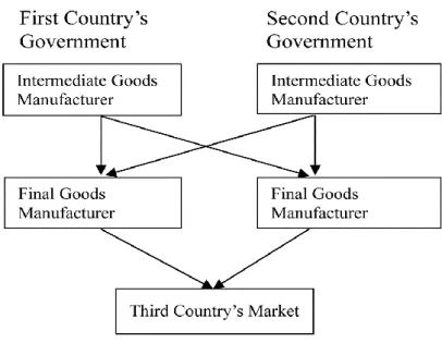
Figure 1 presents the model used in this study. We establish a heterogeneous product model with four companies in three countries. This model has four sets of participants: the governments of Countries 1 and 2, the vendors of intermediate goods of Countries 1 and 2 (upstream industries), the manufacturers of final goods of Countries 1 and 2 (downstream industries), and the consumers of Country 3. Countries 1 and 2 are producing countries, whereas Country 3 is a consuming country. The governments of the two producing countries decide optimal export trade policies. These two countries each have one intermediate goods manufacturer and one final goods manufacturer. The intermediate goods manufacturers each monopolize the production of a crucial intermediate good. The final goods manufacturers must purchase a unit of the intermediate good from the two intermediate goods manufacturers to produce one unit of the final good. The final goods manufacturers in these two countries sell the final goods produced to the third
country.3 The two final goods are heterogeneous products.
Figure 1: The International Trade Structure of Intermediate Goods under Interdependence
This model is implemented in three stages. In the first stage, the governments of the two producing countries consider whether to intervene with exports of the final and intermediate goods or to adopt laissez-faire strategies. The two governments have four decisions in regard to exports: (1) intervene in both intermediate and final goods; (2) intervene in intermediate goods, while adopting laissez-faire for final goods; (3) adopt laissez-faire for intermediate goods, while intervening in final goods; and (4) adopt laissez-faire for both intermediate and final goods. This intervention refers to the government adding quantity taxes or subsidies to exports. The export tax that government i decides to levy on intermediate goods
is si . The export tax that government i decides to levy on final goods is ti.
4
Because the producing country’s welfare is the sum of the upstream and downstream vendors’ profits and the government’s taxes, the objective function of government i
3The conventional literature also typically assumes that the consumers of the producing country do not consume the final goods, which are sold only to the third country as in Brander and Spencer (1985).
4If the variables
i
s and t are positive, this indicates taxation. Negative values indicate i
is as follows. 1 2 1 2 ( , , , ) i i i i j i i W s s t t s q t q . (1)
In this equation, i represents the profit of country i’s intermediate goods
manufacturers, i represents the profit of country i’s final goods manufacturers,
and qi ( q ) represents consumers’ demand for country i’s (j’s) final goods j
(i j, 1, 2, i j).
In the second stage, the intermediate goods manufacturers of the two countries monopolize the production of intermediate goods and set price ai for their own
profits. To simplify the analysis, assume that the production cost of the intermediate goods manufacturers is 0. Although there is no cost difference internationally, it needs to be asked what are the reasons for the division of labor between countries. In actual fact, since only a complementary relationship exists, it then constitutes a “division of labor” economics, without the need for international differences in cost. Because the demand for the two intermediate goods manufacturers’ products is the demand derived from the downstream industries, the profit function of country i’s
intermediate goods manufacturers is as shown in Equation (2). The firm in country i sells the intermediate goods to the foreign country at the same price (i.e.,ai), where
(ais qi) j means that the net profit from the exports is equal to the revenue a q i j
minus taxation s q . i j ( ) i i i i i j a q a s q . (2)
In the third stage, the two countries’ final goods manufacturers combine equal proportions of the two intermediate goods into final goods. Each unit of the intermediate goods can form one unit of the final goods. In the third stage, the final goods manufacturers engage in price competition in the third country, setting the price at pi for their personal profit. To simplify the analysis, assume that the
assembly cost for the final goods manufacturers is 0. Thus, only the costs of purchasing intermediate goods are faced. The profit function of country i’s final goods manufacturers is as follows:
( ) ( )
i
i i i i j i
p t q a a q
. (3)
two countries’ final goods are set as heterogeneous products. This results in the demand function for country i’s final goods being expressed as follows:
i i j
q p p . (4)
In this equation, , , 0. The relationship between the parameters and
represents the degree of substitutability between the two countries’ final products. If 0, this indicates that the two products are stand-alone products. If , this indicates that the two products are entirely substitutes for each other. We assume that
. Therefore, the two final goods have a certain degree of heterogeneity. The product differentiation is crucial for the results obtained in the paper, because we assume that
, which rules out entirely the substitute situation
. In the analysis below, although there are several cases derived in this paper, as shown in Appendices A and B, since the present model does not assume that the size of is greater or smaller than and
, due to the
assumptions, we do not assume the real values of these three variables, and therefore many variables cannot be compared. We will focus on the comparative trade policies, and thereby deduce four propositions.3
□
Optimal Trade Policy
This study’s model involves a three-stage game used to obtain a subgame perfect equilibrium. Backward induction from the final stage should be used to obtain optimal trade policies for the two countries’ governments.
In the third stage, country i’s final goods manufacturers determine final goods prices to maximize their own profits i. Using the two manufacturers’ first-order
conditions simultaneously, we can solve the final goods price as a function of intermediate goods prices and tax rates.
2 1 2 2 2 2 (2 )( ) 4 i j i t t a a p - . (5)
In the second stage, country i’s intermediate goods manufacturers determine intermediate goods prices to maximize their own profits i . Using these two
goods prices are a function of tax rates. 1 2 2 3( ) 6 6 i j i s s t t a . (6)
In the first stage, government i chooses whether to intervene with intermediate and final goods or to adopt laissez-faire policies. If the government decides to intervene, tax or subsidization rates must be determined to maximize the country’s welfare. Therefore, prior to solving the Nash equilibrium entirely, 16 situations can be classified. This is because the two countries’ governments can decide whether to intervene with the trade in intermediate and final goods or to adopt laissez-faire policies. Therefore, each government has four strategies.5 Under these 16 conditions,
the governments select optimal trade policies to pursue their own greatest welfare
i
W . However, prior to the Nash equilibrium, we must understand whether a
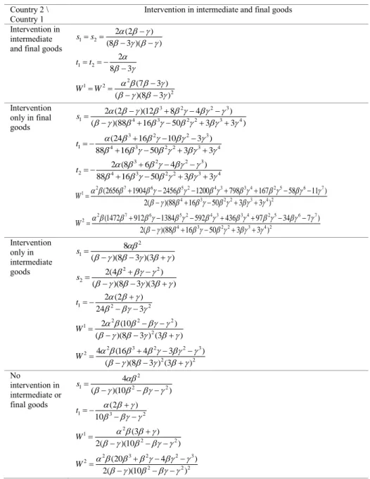
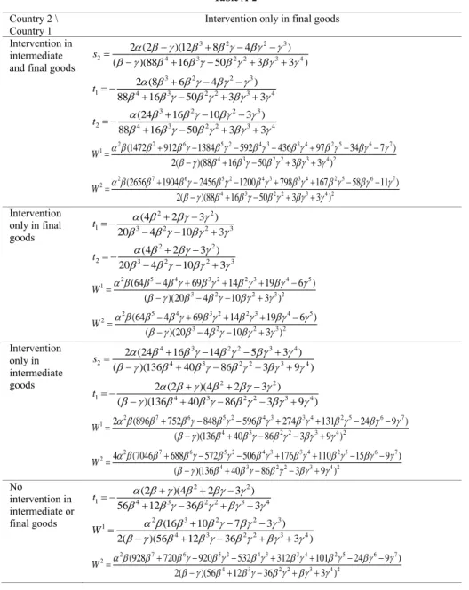
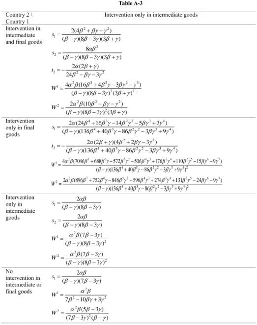
consistent direction exists in the two governments’ decisions to tax or subsidize in these 16 situations. The answer we have obtained for this question is affirmative. The trade policy selections of the two countries in these 16 situations and their welfare are shown in the Appendices. Therefore, we arrive at Proposition 1:
[Proposition 1] The directions in trading policy adopted by the two countries’ governments in the 16 combinations produced when the governments decide whether to intervene with intermediate and final goods exports or to adopt faire policies all conform to the following consistency: taxing or adopting laissez-faire policies for intermediate goods (si 0) and subsidizing or adopting laissez-faire policies for final goods (ti0).6
Equation (6) indicates that a government taxing intermediate goods and subsidizing final goods increases the price of this country’s intermediate goods. Because the intermediate goods are not competing with each other, but have a complementary relationship, the government does not have to use subsidies to increase the competitiveness of intermediate goods. The government taxes
5The four export policies are (1) intervene with both intermediate and final goods; (2) intervene with intermediate goods, and adopt laissez-faire for final goods; (3) adopt laissez-faire for intermediate goods, and intervene with final goods; and (4) adopt laissez-faire for both intermediate and final goods.
6There are 16 cases in Table A-1, Table A-2, Table A-3 and Table A-4. In addition to the first case of Table A-1 being an internal solution of trade policy, the other 15 cases are exogenous corner solutions.
intermediate goods instead. Although this measure increases the unit costs of the country’s final goods manufacturers, it also increases the unit costs for the opposing country’s final goods manufacturers. The negative influence of this on the country’s final goods manufacturers is comparatively moderate,7 and far smaller than the
benefits of the price increase that accrue to the intermediate goods manufacturers.8
In addition, the government’s goal in subsidizing final goods is to create a cost advantage for the country’s final goods, thereby helping strengthen market competition in the third country, and expanding their market in the third country.9
This conclusion is identical to that of Brander and Spencer (1985) in the conventional literature, who investigated only final goods policies.
In the first stage, we found that the two countries were both characterized by stable Nash equilibria in the 16 policy combinations at the disposal of the two governments as they chose whether to intervene in the intermediate and final goods trade. The following proposition can be derived:
[Proposition 2] When the intermediate goods of two countries are entirely complementary and the final goods are heterogeneous products, the two governments’ optimal trading policy is to adopt net taxation for intermediate goods
( * 0
i
s )10 and laissez-faire for final goods ( * 0
i
t ).
This proposition shows that when the international division of labor is increasingly prevalent, the importance of an intermediate goods trade policy may exceed that of the final goods trade policy. This concept discards the conventional thinking that the subsidization of final goods is used to increase competitive strength. This is replaced with intermediate goods taxation to improve welfare. The
7 2 2 2 2 2 2 2 2 1 2 / ( )[4 2 ( )( 2 ) (4 2 8 ) (4 4 2 )] / [18(2 ) i i i j s s s t t (2 )]. 8 2 2 2 2 2 2 2 2 1 2 / [ 8 4 ( )(2 ) (7 11 14 ) (22 7 11 )] / [18(2 ) i i i j s s s t t (2 )].
9 The influence of the government’s policies on the demand for final goods is
2 2 2 2
/ (8 2 4 )(24 6 ) 0
i i
q t
, If ti0, then t is a tax; on the other hand, if i ti0,
then ti is a subsidy. qi/ ti 0 means that subsidizing final goods can expand the market in the third
country.
10The optimal trade policy is * 2 / [( )(8 3 )]
i
primary reason for this transformation in trade policy is the complementarity of intermediate goods and the roles of decision-making and welfare.
However, this equilibrium is not optimal for the two countries.11 If the two
countries change their policies to subsidize only final goods, this is beneficial to both countries.12 This Pareto-improved solution is, however, not an equilibrium
solution. This is because both governments have incentives to tax intermediate goods.13 Even if the two countries add additional taxes to intermediate goods, this
will still not result in an equilibrium. This situation is similar to the prisoner’s dilemma.
4
□
Cooperation Agreement between the Two Governments
Currently, regional economic integration and economic communities are becoming increasingly prevalent. Various nations with close relationships in life or production frequently draw up cooperation agreements on trade issues. In this section, the two originally self-interested trading nations coordinate to facilitate their common interests. Following Section 2, the joint welfare of the two countries can be written as follows:
1 2
1 2 1 2 1 2 1 2 1 2 1 2 1 1 2 2
( , , , ) ( , , , ) ( , , , )
W s s t t W s s t t W s s t t p q p q . (7)
The manufacturers’ decision problems during the second and third stages are identical to those of Section 2. All manufacturers are determining prices to maximize personal profit. During the first stage, the two governments determine s1,
1
t , s2 , and t2 for maximum joint welfare. We can then obtain the following
proposition:
[Proposition 3] When the two governments focus on seeking maximum joint
11In this equilibrium, the welfare of the two countries is 2 (7 3 ) / [(8 3 ) ( 2 )]. 12At this time, the two countries can subsidize only final goods. Their welfare is as follows: 2 (4 2 2 )(162 3 5 2 8 2 3 ) / [(3 )(20 3 4 2 10 2 3 ) ]3 2
.
13In the original equilibrium, if one country betrays the equilibrium and adds additional taxes to intermediate goods, the welfare of the betraying country will increase as follows:
2 7 6 5 2 4 3 3 4 2 5 6 7 4 3
2 (896 752 848 596 274 131 24 9 ) / [( )(136 40
2 2 3 4 2
86 3 9 ) ] 0
welfare, they formulate the following trade policy: the final goods trade policies of the two countries are identical. All intermediate and final goods policy variables are mutually interchangeable and the total effect is subsidization. The variables can be expressed as follows: t1t2 and s1 s2 t1 t2 (4 3 ) / [ ( )]0.
14
This proposition shows that when the two countries jointly establish optimal trade policies, all intermediate and final goods trade policies are entirely mutually replaceable. Regardless of how these four trade policies are switched, upstream and downstream vendor profits, the two countries’ total welfare, and final goods prices are not affected.15 This shows that the two governments do not require excuses to
subsidize or levy taxes as long as subsidizations are focused on a certain country’s final goods or intermediate goods trade policy. However, this cooperative solution is unstable. The two governments have incentives to adopt net taxation.16 Agreements
must be established for enforcement. Even with mandatory enforcement on fairness principles, an agreement must eventually be reached: s1s2 , t1t2 , and
(4 3 ) / [2 ( )]
i i
s t . We obtain si ti 0 , which refers to net subsidization under an agreement. Given that welfare is maximized without intervention in theory, why should siti not be equal to 0? This is because the two
countries are both export-oriented. However, if one country is export-oriented and the other is import-oriented, the optimal trade policy under the agreement is the free trade policy (i.e., si ti 0).
5
□
Intermediate Goods Market With a Monopoly and
Competition Coexisting
14Although international cooperation in production can lead to one country producing the intermediate goods with the other producing the final goods in other models, there does not necessarily need to be complementary production between the two countries, since a single country alone can integrate intermediate goods and final goods in the vertical integration of production.
15The upstream manufacturers’ profits are 2
/ (4 )
. The downstream manufacturers’ profits are 2
(2 ) / [2 ( )]
. The two countries’ total welfare is 2
/ [2( )]
. The final goods price is / [2( )]
.
16At this time, Country i’s welfare i 2(5 3 ) / [4 ( )] ( ) / 2
i i
W st is a monotonically increasing function ofsiti.
Suppose that one of the producing countries opens its intermediate goods market to perfect competition. The government’s trade policy is to no longer intervene in this market. The other country’s intermediate goods market, by contrast, remains a monopoly. This section examines how the optimal trade policies of the two producing countries change when their intermediate goods are in this type of asymmetric market structure.
When Country 2’s intermediate goods are in perfect competition and trade policy no longer intervenes, then a20 and s20. With this exception, the other structures are all identical to the basic model in Section 2. By using reverse induction in the first stage, the final goods manufacturers establish final prices to maximize their own profits (Equation (3)). The optimal equilibrium price is shown in Equation (5). The results of this response function are brought back to the second stage. The intermediate goods manufacturers set final prices to maximize their own profits (Equation (2)). We can obtain Country 1’s optimal intermediate goods price as follows: 1 1 2 1 2( ) 4 4 s t t a
. (8)Equations (5) and (8) with optimized conditions are brought back to the first stage to examine whether the two governments adopt trade policies in pursuit of their own welfare (Equation (1)). This topic’s subgame perfect equilibrium can be inferred. Thus, we put forward the following proposition:
[Proposition 4] If the two intermediate goods market structures change, Country 1’s remains a monopoly and Country 2’s changes to perfect competition. Therefore, the two governments have the following optimal export trade policy: Country 1’s government adopts subsidization trade policies for intermediate and final goods (s10 and t10), and Country 2 levies taxes on the final goods trade (t2 0).
When Country 2’s intermediate goods market is transformed from a monopoly to perfect competition, Country 1’s optimal policy is to adopt subsidization and not taxation for intermediate goods. The government of Country 2’s optimal policy is to tax final goods and not to adopt laissez-faire or subsidization policies. This result conflicts with those of previous studies and even the conventional literature. We
reflect further on this result.
We first address the intermediate goods trade policy. In the model in Section 3, the two countries’ market structures are symmetrical. In addition, the pricing of the intermediate goods is strategically replaceable. 17 Therefore, if Country 1’s
government adopts subsidization strategies for intermediate goods, Country 1’s intermediate goods prices will be reduced and Country 2’s intermediate goods prices will increase. 18 However, Country 2’s intermediate goods market is now
characterized by perfect competition. The two intermediate goods no longer interact in terms of price.19 Equations (1), (2), and (3) show that the welfare of Country 1’s
government is 1 1 2 1 2 ( , , , ) W s s t t 1 1 1 2 s q t q1 1 [a q1 1 (a1s q1) 2] [(p1t q1) 1(a1a q2) 1] s q1 2 t q1 1 (p1a q2) 1 a q1 2. Therefore, the inference from the differences in the 2 models described shows that the subsidization policies produce greater unfavorable factors in the former model. Therefore, Country 1’s government has more (less) of an incentive to subsidize (tax) in the latter model (e.g., the first case in Table B-1 in the appendix: s1
2 [ (2 )(2 ) ]/ 2
[ 2
(14 2
5 )] 0) than in the former model (e.g., the first case in Table A-1 in the appendix:s1 [2 (2 )]/[(83 )( )]0).
This study examines the final goods trade policy. In the model in Section 3, the two countries are symmetrical in terms of their market structure. If Country 2’s government adopts taxation policies on final goods, then the costs faced by the final goods manufacturers increase, which raises final goods prices. This reduces the demand for final goods and also decreases the derived demand for intermediate goods. Country 2’s intermediate goods market is now characterized by perfect competition. However, taxation policy can influence only the demand for final goods. It does not influence the profits of intermediate goods manufacturers. Therefore, Country 2’s government has more (less) of an incentive to tax (subsidize) in the latter model (e.g., the first case in Table B-1 in the appendix: t2
2 2
[ (2 )]/ 2 2
[ (14 5 )]0) than in the former model (e.g., the first case in Table A-1 in the appendix: t2 2/[83 ] 0.).
17When the final goods manufacturers engage in price competition,
/ 2 ( ) / (2 ) 0
i i j
a a . 18Equation (6) shows that
1/ 1 1 / 3
da ds and da2/ds1 1/ 6. 19
2 0
6
□
Conclusion
This study investigates optimal trade policies where intermediate goods are characterized by an international division of labor. When examining trade policies, previous studies failed to consider intermediate goods in the international division of labor. Because this is a common phenomenon, we analyzed the influence of internationally interdependent intermediate goods on the overall trade strategy. In addition, we also investigated the influence of changes in the market structure of the intermediate goods on the optimal trade policy.
We established a model with two intermediate goods monopolized by upstream manufacturers in two countries with oligopolistic final goods market structures. This model was used to investigate the influence of the international division of labor on the two governments’ trade policies when the intermediate goods are entirely complementary internationally and the final goods markets are characterized by imperfect competition. This study first used the linear demand function in which the upstream and downstream market structures of the producing countries are symmetrical, and the intermediate goods manufacturer costs are standardized to 0. We obtained the following preliminary main results. First, when intermediate goods manufacturers from two countries monopolize two intermediate goods and the two countries’ governments must first choose whether to intervene in the trade in intermediate and final goods, the two governments will abandon final goods trade policies in equilibrium. Instead, they will adopt taxation trade policies on only intermediate goods. Second, in addition to the government’s optimal strategy being to tax intermediate goods, if the two governments engage in levying additional taxes on the final goods, then the welfare of the two countries will increase. This is not at the equilibrium point, but if the two governments can formulate a contract, it can increase the welfare of both parties. We found that this contract adopts net subsidization on the sum of intermediate and final goods trade policies. Finally, by changing the originally symmetrical intermediate goods market structure of one country to a structure with perfect competition, we found that that country’s optimal trade policy for final goods is to tax. The other country’s optimal trade policy for intermediate and final goods is to subsidize.
Appendix
A.
□
Decision Making and Welfare of Two Countries in
Intermediate and Final Goods Trade Policy
Table A-1
Country 2 \
Country 1 Intervention in intermediate and final goods
Intervention in intermediate and final goods
1 2 2 (2 ) (8 3 )( ) s s 1 2 2 8 3 t t 2 1 2 2 (7 3 ) ( )(8 3 ) W W Intervention only in final goods 3 2 2 3 1 4 3 2 2 3 4 2 (2 )(12 8 4 ) ( )(88 16 50 3 3 ) s 3 2 2 3 1 4 3 2 2 3 4 (24 16 10 3 ) 88 16 50 3 3 t 3 2 2 3 2 4 3 2 2 3 4 2 (8 6 4 ) 88 16 50 3 3 t 2 7 6 5 2 4 3 3 4 2 5 6 7 1 4 3 2 2 3 4 2 (2656 1904 2456 1200 798 167 58 11 ) 2( )(88 16 50 3 3 ) W 2 7 6 5 2 4 3 3 4 2 5 6 7 2 4 3 2 2 3 4 2 (1472 912 1384 592 436 97 34 7 ) 2( )(88 16 50 3 3 ) W Intervention only in intermediate goods 2 1 8 ( )(8 3 )(3 ) s 2 2 2 2(4 ) ( )(8 3 )(3 ) s 1 2 2 2 (2 ) 24 3 t 2 2 2 1 2 2 (10 ) ( )(8 3 ) (3 ) W 2 3 2 2 3 2 2 2 4 (16 4 3 ) ( )(8 3 ) (3 ) W No intervention in intermediate or final goods 2 1 2 2 4 ( )(10 ) s 1 3 2 (2 ) 10 t 2 1 2 2 (3 ) 2( )(10 ) W 2 3 2 2 3 2 2 2 2 (20 4 ) 2( )(10 ) W
Table A-2
Country 2 \ Country 1
Intervention only in final goods Intervention in
intermediate and final goods
3 2 2 3 2 4 3 2 2 3 4 2 (2 )(12 8 4 ) ( )(88 16 50 3 3 ) s 3 2 2 3 1 4 3 2 2 3 4 2 (8 6 4 ) 88 16 50 3 3 t 3 2 2 3 2 4 3 2 2 3 4 (24 16 10 3 ) 88 16 50 3 3 t 2 7 6 5 2 4 3 3 4 2 5 6 7 1 4 3 2 2 3 4 2 (1472 912 1384 592 436 97 34 7 ) 2( )(88 16 50 3 3 ) W 2 7 6 5 2 4 3 3 4 2 5 6 7 2 4 3 2 2 3 4 2 (2656 1904 2456 1200 798 167 58 11 ) 2( )(88 16 50 3 3 ) W Intervention only in final goods 2 2 1 3 2 2 3 (4 2 3 ) 20 4 10 3 t 2 2 2 3 2 2 3 (4 2 3 ) 20 4 10 3 t 2 5 4 3 2 2 3 4 5 1 3 2 2 3 2 (64 4 69 14 19 6 ) ( )(20 4 10 3 ) W 2 5 4 3 2 2 3 4 5 2 3 2 2 3 2 (64 4 69 14 19 6 ) ( )(20 4 10 3 ) W Intervention only in intermediate goods 4 3 2 2 3 4 2 4 3 2 2 3 4 2 (24 16 14 5 3 ) ( )(136 40 86 3 9 ) s 2 2 1 4 3 2 2 3 4 2 (2 )(4 2 3 ) ( )(136 40 86 3 9 ) t 2 7 6 5 2 4 3 3 4 2 5 6 7 1 4 3 2 2 3 4 2 2 (896 752 848 596 274 131 24 9 ) ( )(136 40 86 3 9 ) W 2 7 6 5 2 4 3 3 4 2 5 6 7 2 4 3 2 2 3 4 2 4 (7046 688 572 506 176 110 15 9 ) ( )(136 40 86 3 9 ) W No intervention in intermediate or final goods 2 2 1 4 3 2 2 3 4 (2 )(4 2 3 ) 56 12 36 3 t 2 3 2 2 3 1 4 3 2 2 3 4 (16 10 7 3 ) 2( )(56 12 36 3 ) W 2 7 6 5 2 4 3 3 4 2 5 6 7 2 4 3 2 2 3 4 2 (928 720 920 532 312 101 24 9 ) 2( )(56 12 36 3 ) W
Table A-3
Country 2 \ Country 1
Intervention only in intermediate goods Intervention in
intermediate and final goods
2 2 1 2(4 ) ( )(8 3 )(3 ) s 2 2 8 ( )(8 3 )(3 ) s 2 2 2 2 (2 ) 24 3 t 2 3 2 2 3 1 2 2 4 (16 4 3 ) ( )(8 3 ) (3 ) W 2 2 2 2 2 2 (10 ) ( )(8 3 ) (3 ) W Intervention only in final goods 4 3 2 2 3 4 1 4 3 2 2 3 4 2 (24 16 14 5 3 ) ( )(136 40 86 3 9 ) s 2 2 2 4 3 2 2 3 4 2 (2 )(4 2 3 ) ( )(136 40 86 3 9 ) t 2 7 6 5 2 4 3 3 4 2 5 6 7 1 4 3 2 2 3 4 2 4 (7046 688 572 506 176 110 15 9 ) ( )(136 40 86 3 9 ) W 2 7 6 5 2 4 3 3 4 2 5 6 7 2 4 3 2 2 3 4 2 2 (896 752 848 596 274 131 24 9 ) ( )(136 40 86 3 9 ) W Intervention only in intermediate goods 1 2 ( )(8 3 ) s 2 2 ( )(8 3 ) s 2 1 2 (7 3 ) ( )(8 3 ) W 2 2 2 (7 3 ) ( )(8 3 ) W No intervention in intermediate or final goods 1 2 ( )(7 3 ) s 2 1 2 2 7 10 3 W 2 2 2 (5 3 ) (7 3 ) ( ) W
Table A-4
Country 2 \ Country 1 No intervention in intermediate or final goods Intervention in
intermediate and final goods 2 2 2 2 4 ( )(10 ) s 2 3 2 (2 ) 10 t 2 3 2 2 3 1 2 2 2 (20 4 ) 2( )(10 ) W 2 2 2 2 (3 ) 2( )(10 ) W Intervention only in final goods 2 2 2 4 3 2 2 3 4 (2 )(4 2 3 ) 56 12 36 3 t 2 7 6 5 2 4 3 3 4 2 5 6 7 1 4 3 2 2 3 4 2 (928 720 920 532 312 101 24 9 ) 2( )(56 12 36 3 ) W 2 3 2 2 3 2 4 3 2 2 3 4 (16 10 7 3 ) 2( )(56 12 36 3 ) W Intervention only in intermediate goods 2 2 ( )(7 3 ) s 2 1 2 (5 3 ) (7 3 ) ( ) W 2 2 2 2 7 10 3 W No intervention in intermediate or final goods 2 1 2 (5 3 ) 9( )(2 ) W 2 2 2 (5 3 ) 9( )(2 ) W
B.
□
Decision Making and Welfare of Two Countries in the
Intermediate and Final Goods Trade Policy When the Second
Country’s Intermediate Goods Market is in Perfect Competition
and Government Trade Policy Does Not Intervene
Table B-1
Country 2 \ Country 1 Intervention in intermediate and final goods Intervention in final goods 2 1 2 2 2 (2 )(2 ) (14 5 ) s 3 2 2 3 1 2 2 2 (6 5 3 ) (14 5 ) t 2 2 2 2 2 (2 ) (14 5 ) t 2 5 4 3 2 2 3 4 5 1 2 2 2 (268 176 205 91 45 7 ) 4 ( )(14 5 ) W 2 4 3 2 2 3 4 2 2 2 2 (60 4 37 2 3 ) 4 (14 5 ) W No intervention in final goods 1 2 (2 ) 4 s 1 2 (2 ) 4 t 2 1 (3 ) 8 ( ) W 2 2 16 W
Table B-2
Country 2 \ Country 1 Intervention in only final goods
Intervention in final goods 5 4 3 2 2 3 4 5 1 3 2 2 3 3 2 2 3 (80 68 64 47 14 5 ) (16 10 5 )(10 3 4 ) t 2 2 3 2 2 3 2 3 2 2 3 3 2 2 3 (2 )(8 2 3 ) (16 10 5 )(10 3 4 ) t 2 2 2 9 8 7 2 6 3 5 4 4 5 3 6 2 7 8 9 1 3 2 2 3 2 3 2 2 3 2 (6 3 )(5760 5632 6392 5428 2742 1465 506 88 12 3 ) 4(16 10 5 ) (10 3 4 ) W 2 2 2 2 2 3 2 2 3 2 2 3 2 2 3 3 2 2 3 (6 3 )(10 )(8 2 3 ) (16 10 5 )(10 3 4 ) W No intervention in intermediate or final goods 2 2 1 4 3 2 2 4 2 (2 )(6 3 ) 44 12 25 t 2 3 2 2 3 1 4 3 2 2 4 (16 10 7 3 ) ( )(44 12 25 ) W 2 3 2 2 3 2 2 4 3 2 2 4 (8 2 3 ) ( )(44 12 25 ) W Table B-3 Country 2 \ Country 1
Intervention only in intermediate goods Intervention in final goods 3 2 2 3 1 4 3 2 2 3 4 (16 10 5 ) (22 5 11 ) s 2 2 2 4 3 2 2 3 4 (2 )(2 ) (22 5 11 ) t 2 7 6 5 2 4 3 3 4 2 5 6 7 1 4 3 2 2 3 4 2 (592 560 432 376 111 69 7 5 ) 4( )(22 5 11 ) W 2 2 2 2 2 2 2 4 3 2 2 3 4 2 (2 ) (6 3 )(10 3 ) 4( )(22 5 11 ) W No intervention in intermediate or final goods 1 2 3 s 2 1 ( )(3 ) W 2 2 2 (3 ) W
Table B-4
Country 2 \ Country 1
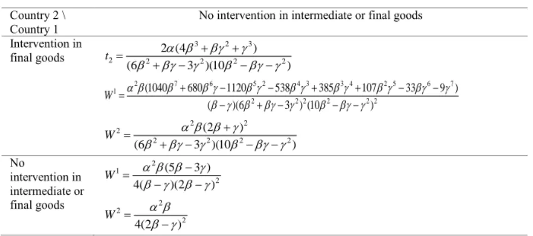
No intervention in intermediate or final goods Intervention in final goods 3 2 3 2 2 2 2 2 2 (4 ) (6 3 )(10 ) t 2 7 6 5 2 4 3 3 4 2 5 6 7 1 2 2 2 2 2 2 (1040 680 1120 538 385 107 33 9 ) ( )(6 3 ) (10 ) W 2 2 2 2 2 2 2 (2 ) (6 3 )(10 ) W No intervention in intermediate or final goods 2 1 2 (5 3 ) 4( )(2 ) W 2 2 2 4(2 ) W
References
Brander, J. A. and B. J. Spencer, (1985), “Export Subsidies and International Market Share Rivalry,” Journal of International Economics, 18, 83-100.
Chang, W. W. and J. C. Kim, (1989), “Competition in Quality-differentiated Products and Optimal Trade Policy,” Keio Economic Studies, 26, 1-17.
Economides, N., (1989), “Desirability of Compatibility in the Absence of Network Externalities,” The American Economic Review, 79, 1165-1181.
Hecking, H. and T. Panke, (2014), “Quantity-setting Oligopolies in Complementary Input Markets - The Case of Iron Ore and Coking Coal,” Technical Report, Energiewirtschaftliches Institut an der Universitaet zu Koeln.
Matsushima, N. and T. Mizuno, (2012), “Profit-enhancing Competitive Pressure in Vertically Related Industries,” Journal of the Japanese and International
Economies, 26, 142-152.
Matsushima, N. and T. Mizuno, (2013), “Vertical Separation as a Defense against Strong Suppliers,” European Journal of Operational Research, 228, 208-216. Matutes, C. and P. Regibeau, (1988), “‘Mix and Match’: Product Compatibility
without Network Externalities,” RAND Journal of Economics, 19, 221-234. Reisinger, M. and E. Tarantino, (2013), “Vertical Integration with Complementary
Inputs,” TILEC Discussion Paper No. 2011-004, SSRN eLibrary.
Policy,” The Review of Economic Studies, 58, 153-170.
Spencer, B. J. and R. W. Jones, (1992), “Trade and Protection in Vertically Related Markets,” Journal of International Economics, 32, 31-55.