有通道估計誤差下之多天線信號偵測

國 立 交 通 大 學

電信工程研究所

碩 士 論 文

有通道估計誤差下之多天線信號偵測

MIMO Signal Detection in the Presence of

Channel Estimation Errors

研 究 生：林玉婷

指導教授：蘇育德 博士

有通道估計誤差下之多天線信號偵測

MIMO Signal Detection in the Presence of

Channel Estimation Errors

研究生：林玉婷

Student : Yu-Ting Lin

指導教授：蘇育德 博士 Advisor : Dr. Yu T. Su

國 立 交 通 大 學

電 信 工 程 研 究 所

碩 士 論 文

A Thesis

Submitted to Institute of Communications Engineering

College of Electrical and Computer Engineering

National Chiao Tung University

in Partial Fulfillment of the Requirements

for the Degree of Master of Science

in Communications Engineering

October 2010

Hsinchu, Taiwan, Republic of China

有通道估計誤差下之多天線信號偵測

研究生：林玉婷 指導教授：蘇育德 博士

國立交通大學電信工程學系碩士班

中文摘要

相較於傳統的單輸入單輸出(SISO)系統，使用多傳送與接收天線的

多 輸 入 多 輸 出 (MIMO) 的 無 線 通 訊 系 統 可 大 幅 的 增 加 系 統 容 量

(capacity)，因此在過去十年被廣泛的研究，相關技術並已應用於實際系

統成為國際無線通訊標準規格不可或缺的一部份。大多數對於MIMO訊

號偵測的研究，都假設接收端有百分之百正確的通道資訊(CSI)，但實際

上，這是不可能的。通道資訊需透過某種估計演法得到，誤差在所難免，

而基於此不正確CSI所偵測的數據之可靠性也必須打折扣。事實上許多

研究都顯示接受器的效能將有顯著的降低。因此，如何在設計MIMO接

收器時將通道估計誤差一併考慮以盡量減少因上述CSI不匹配的因素造

成的效能損失是一項相當迫切的課題，也是本文的主要研究動機。我們

首先探討通道估計誤差對兩種MIMO信號偵測法­即粒子群趨動交叉熵

偵測法及QRD-M偵測法­的性能之影響。

粒子群趨動交叉熵法（

）偵測法是

在給定接收向量後，試圖尋找傳送信號位置的事後機率分布。這個機率

分布是藉由在接收向量附近取樣並且反覆的更新使得機率分佈擁有最

小交叉熵（相較於現有的機率分佈）。為了改善效能，粒子群趨動的概

念則被引入來提供一組新的機率分布。另一方面，QRD-M則是一個以樹

狀結構為基礎的低複雜度偵測法。在少許效能損失下，利用樹狀結構搜

尋並且減少每一層的存活路徑。

由於最小歐式距離偵測法在有通道估計誤差的情形下對於前述兩

個偵測器並不適用，我們提出考量通道估計誤差效應的新型最佳偵測結

構，提出了新的解碼度量(decoding metric)。模擬結果顯示新法雖然增加

了些許計算複雜度但卻有顯著的效能提昇。我們也發現將同樣的度量應

用在有時空編碼的MIMO系統亦可得到類似的改善。

MIMO Signal Detection in the presence of Channel

Estimation Errors

Student : Yu-Ting Lin Advisor : Yu T. Su

Institute of Communications Engineering National Chiao Tung University

Abstract

The multiple-input multiple output (MIMO) technology promises significant capac-ity increase over conventional single-input single-output systems. Most investigations on MIMO signal detection, however, assume perfect channel state information (CSI), which is difficult, if not impossible, to realize in practice. Earlier studies have shown that that the performance of MIMO detection schemes will suffer from severe degradation in the presence of channel estimation errors.

In this thesis, the effects of imperfect CSI on two MIMO signal detectors, namely, the Particle-Swarm-Driven Cross-Entropy (PSD-CE) based detector and the QRD-M detector, are studied, and new detector structures that take into account the CSI error are proposed.

The PSD-CE detector tries to estimate and refine the ‘a posteriori probability dis-tribution’ of the transmitted signal location given the received vector. The distribution is estimated by sampling over the neighborhood of the received vector and is iteratively updated to the one which has the minimum cross entropy with respect to the current distribution. It is further modified by applying the concept of Particle Swarm Optimiza-tion to render a mixture of probability distribuOptimiza-tion. QRD-M, on the other hand, is an efficient tree-search based detector. It prunes the search tree to reduce the number of surviving paths with minimum performance loss.

Since the minimum Euclidean distance criterion is no longer suitable for both de-tectors in the presence of channel estimation errors, the proposed MIMO dede-tectors take into account the imperfect CSI effect by averaging the estimation errors to obtain a new decoding metric. Numerical examples are given to demonstrate the performance improvement which is attained with insignificant complexity increase.

Acknowlegements

I am truly grateful to my advisor, Professor Y. T.Su. This thesis would not have been possible without his guidance and support. His wisdom and encouragements guided me not only in the research for this thesis, but also in my daily life. It is really an honor to be his student.

I am greatly indebted to my seniors, Jen-Yang and Chang-Ming. They helped me in times of trouble and gave me many suggestions during the years. The knowledge I gained from the many discussions we had over the past two years is invaluable.

I would also like to thank the members of lab 811, they have always been there for me, giving me encouragements and advises in times of need. I will always remember the sharing of our week in the meetings.

Finally, I wish to express my heartfelt gratitude to my dearest family for their spiri-tual support and unconditional love.

Contents

Chinese Abstract i

English Abstract ii

Acknowledgement iv

Contents v

List of Tables vii

List of Figures viii

1 Introduction 1

2 System Model 5

2.1 MIMO Systems with Perfect Channel Estimation . . . 5 2.2 Pilot-Based Channel Estimation . . . 7

3 A Review of MIMO Detectors 10

3.1 Maximum Likelihood Detector . . . 10 3.2 Zero-Forcing (ZF) Detector . . . 10 3.3 The QRD-M Detector . . . . 11

4 Particle-Swarm-Driven Cross-Entropy MIMO Detector 14

4.2 Particle Swarm Optimization . . . 16

4.3 Improving the PSD-CE Detector . . . 17

5 Signal Detection With CSI Uncertainty 20 5.1 Effects of Channel Estimation Error . . . 20

5.2 QRD-M detection with imperfect CSI . . . . 22

6 Space Time Code 24 6.1 Background . . . 24

6.2 Alamouti Space-Time Block Code . . . 24

6.3 Hamming based Space-Time Block Code . . . 27

7 Simulation Results 29 7.1 Performance Comparison with Perfect CSI . . . 29

7.2 Performance in the Presence of CSI Error . . . 31

7.2.1 Spatial multiplexing system . . . 32

7.2.2 Alamouti space-time coded system . . . 35

7.2.3 Hamming coded system . . . 35

8 Conclusion 37

List of Tables

List of Figures

2.1 A MIMO system model. . . 5 3.1 Tree structure of QRD-M (M = 4), NT = 3, NR = 3, with 4-QAM

modulation. . . 13 7.1 Comparison of the BER performance of the modified PSD-CE detector

(3 iterations and 60 samples/iteration) and other known detectors in a MIMO system with NT = NR= 4 using 4-QAM. . . 30

7.2 Comparison of the BER performance of the conventional PSD-CE detec-tor and the modified PSD-CE in a MIMO system with NT = NR = 4

using 16-QAM. solid line : 5 iterations and 500 samples/iteration; dashed line : 3iterations and 500 samples/iteration. . . 31 7.3 Effect of channel estimation errors on the system performance. . . 32 7.4 Effect of channel estimation errors on a 2 × 2 MIMO with T = 2 using

BPSK. . . 33 7.5 Effect of channel estimation errors on a 2 × 2 MIMO with T = 4 using

BPSK. . . 33 7.6 The use of PSDCE detector under channel estimation errors in a 2 × 2

MIMO with T = 2 using BPSK. . . . 34 7.7 The use of PSDCE detector under channel estimation errors in a 2 × 2

7.8 Employing Alamouti code in a 2 × 2 systme with estimation errors with

T = 4 using 16-QAM. . . . 35 7.9 Employing Alamouti code in a 2 × 2 systme with estimation errors with

Chapter 1

Introduction

Multiple-input and multiple-output (MIMO) technologies have gained enormous popularity in the recent years because the significant communication capacity enhance-ment they promised to deliver [1], [3]. A MIMO system uses multiple antennas at both the transmit and the receive ends. In a rich-scattering MIMO channel that can be characterized by a channel matrix with independent and identically distributed (i.i.d.) Rayleigh entries, the associated capacity can increase linearly with the minimum of the number of transmit and receive antennas [2].

However, such a capacity increase can only be realized if the channel matrix is per-fectly known. The more practical concern of detecting MIMO signals has been answered by many alternatives, e.g. the Zero Forcing (ZF) [4] detector and V-BLAST [6] detector. Like the capacity issue, these detection schemes perform well only if the channel state information (CSI), i.e., the channel matrix, is perfectly known at the receiver [7]. In practical situations, the knowledge of the channel is never perfect and is attained by some channel estimation scheme at the receiver. The most popular and practical way to obtain the CSI at the receiver (CSIR), is to insert known sequences of symbols, often referred to as pilot signals, within the transmit data stream to aid channel estimation [8], [9]. Information symbols are then detected as though the estimated channel matrix is perfect. Due to the finite number of pilot symbols and various sources of noise and interference, the receiver can only obtain imperfect estimates of the channel. As a result,

such a mismatched detector is a sub-optimal approach and its performance is severely degraded in the presence of channel estimation errors as shown in [8] and [10].

The optimum detection method in MIMO systems is the Maximum Likelihood (ML) detector which often calls for exhaustive search over the entire set of possible transmitted symbol vectors. Apparently, the major drawback of ML detector is its high complexity that increases exponentially with the number of transmit antennas and modulation size of the constellation. On the other hand, when perfect CSI is not available, the minimum Euclidean distance criterion is no longer an ML one. To find an ML detection metric, many investigations [20], [22], assume that the channel (matrix) is uncorrelated with the channel estimation error (matrix). This is not appropriate if we recall that both the least-squares (LS) and minimum mean square error (MMSE) channel estimators follows the orthogonal principle which says that the estimation error should be orthogonal to the estimator in some sense. Based on this observation we adopt a different model and derive a new detection metric based on the latter assumption.

In our work, we consider two MIMO detection schemes: the Particle-Swarm-Driven Cross-Entropy (PSD-CE) [11] method and the M-algorithm combined with QR de-composition (QRD-M) [12], [13]. Both schemes have comparatively low complexities compared with the ML detector.

The PSD-CE is a Monte Carlo based stochastic approach that attempts to find the transmitted symbol. It is an iterative method that tries to approach the ‘optimal probability distribution’ of the transmitted signal. It generates samples over the entire neighborhood of the received vector with uniform distribution. Then the probability distribution of the samples is updated with the ‘better’ samples. After some iterations, the probability distribution should close in on the optimal distribution in the Cross-Entropy (CE) sense [14]. To improve the performance further, the concept of Particle Swarm Optimization (PSO) [16], [17] is added.

some changes to the original PSD-CE method. Going over the steps of PSD-CE, we realize that initializing the probability distribution with uniform distribution means be-ginning the search without any information. Instead of starting the search in such an inefficient manner, we could try to use some information that can be easily obtained by some other simple methods, Zero Forcing for example. By changing the initial distribu-tion so that it contains some useful informadistribu-tion, the modified PSD-CE method becomes more efficient, bearing better performance than the conventional PSD-CE with lower computational complexity.

Unlike the PSD-CE method, QRD-M is a deterministic detection algorithm. Dif-ferent from the QR detection [21], QRD-M is a tree search algorithm [13], [21]. The concept of QRD-M is to apply the tree search to detect symbols in a sequential man-ner. Instead of making a decision for the symbols at each detection level as in the QR detection method, QRD-M retains M reliable paths. Decision is made only after all the layers have been processed. It can achieve near-ML performance with relatively low but fixed complexity. There is a trade-off between the complexity and performance on the selection of M. With a large M, better performance is achieved at the cost of higher complexity. Usually, M is set to be the size of the modulation constellation.

The new optimization criterion mentioned earlier is used in place of the original criterion ky − Hxk2 _{in the PSD-CE method. However, it cannot be directly applied to}

the QRD-M algorithm because it can no longer be decomposed into the sum of separate branch metrics, as will be shown in Chapter 5. We figured out a way such that the new criterion becomes the lower bound and can be used in the QRD-M method to achieve better performance in the presence of channel estimation errors.

By employing some simple space-time block codes (STBC) [18], [19], the effects of the gain in the modified ML criterion is apparent. G. Taricco et al. [20] examines space-time decoding with imperfect channel estimations, but their analysis is based on the assumption that the channel estimation error is orthogonal to the channel.

The rest of this thesis is organized as follows: in Chapter 2 we describe the system model used and the main assumptions concerning channel estimation. In Chapter 3 we review some existing MIMO detection schemes that are of interest to our study. Chapter 4 gives a detailed description of the PSD-CE algorithm, as well as the modifications made to improve its performance. We then propose improved detectors in the presence of channel estimation errors in Chapter 5. Space-Time codes are introduced in Chapter 6. Simulation results are given in Chapter 7 and finally, Chapter 8 gives the conclusion. The following notations are used throughout the thesis: upper case bold symbols denote matrices and lower case bold symbols denote vectors. IN is a N × N identity

matrix. The superscripts (·)T_{, (·)}H _{and (·)}†_{represent the transpose, Hermitian transpose}

and the pseudo-inverse, respectively. E{·} denotes the statistical expectation, tr(·) is the trace of a square matrix.

Chapter 2

System Model

2.1

MIMO Systems with Perfect Channel

Estima-tion

We consider a MIMO system [1] with NT transmit antennas and NR receive

anten-nas. As shown in Fig. 2.1, data is demultiplexed into NT data substreams, then the

substreams are mapped onto sequences of M-QAM symbols where the signal constella-tion is denoted by AM. These symbol sequences are transmitted over the NT antennas

simultaneously. T R,N N

h

h

h

h

y

Transmitter Receiver

Detector Estimated data Input data 1 n R N n

If T consecutive signal vectors are transmitted, the transmitted signal can be rep-resented as an NT × T matrix X, where X , [x1, . . . xT] and xt is the signal vector

transmitted at the tth time slot. The signal vector transmitted at the tth time slot xt

can be represented as

xt= [x1,t, . . . , xNT,t]

T _{∈ A}NT

M (2.1)

Similarly, assuming perfect timing receiver and quasi-static channel , the correspond-ing NR× T received signal matrix, Y, can be expressed as

Y = HX + Z (2.2) where Y = [y1, . . . , yT] (2.3) Z = [z1, . . . , zT] (2.4) and yt= [y1,t, . . . , yNR,t] T _{∈ C}NR _(2.5) zt= [z1,t, . . . , zNR,t] T _{∈ C}NR (2.6) H =      h1,1 h1,2 · · · h1,NT h2,1 h2,2 · · · h2,NT ... ... . .. ... hNR,1 hNR,2 · · · hNR,NT     ∈ C NR×NT (2.7)

Here, C denotes the complex-valued domain. H describes the overall NR× NT channel

matrix, the (j, i)th element of H, hj,i, is the channel response between the ith transmit

antenna and the jth receive antenna. In this thesis, the elements of H are independently and identically distributed (i.i.d.) zero-mean complex Gaussian random variables with unit variance. Z is the NR× T additive white Gaussian noise (AWGN) matrix observed

at receiver. Each element of Z has zero mean and variance σ2

z, while the average transmit

power of each antenna is normalized to one. Hence, we have Es, 1 NT T E [ k X k2_{] =} 1 NT T E [ tr { XXH_{} ] = 1 (2.8)}

and

E{ ZtZHt } = σ2zINR. (2.9)

where tr denotes the trace operation, IN is an identity matrix of size N × N and t =

1, · · · , T .

2.2

Pilot-Based Channel Estimation

The channel information is estimated at receiver and it is often assumed to be perfectly estimated in a lot of literature. However, due to the time-varying channels and quan-tization errors, only an estimate of the channel matrix that is corrupted by estimation errors is available at the receiver side and the assumption about perfect estimate is not rational in a practical system.

For pilot-based channel estimation scheme, a pilot matrix, XP, is sent and the receiver

observes

YP = HXP + ZP (2.10)

where ZP is the noise matrix affecting the transmission of the pilot symbols. XP is a

known NT × P matrix at receiver with average pilot symbol energy

Ep , 1 NT P k XPk2 = 1 NT P tr { XP XHP} (2.11)

Since the number of the elements of H is NRNT, at least NRNT independent

mea-surements are needed to estimate the NR×NT channel matrix. To satisfy this condition,

NR measurements are observed in each time slot and we require P to be larger than or

equal to NT. Furthermore, in order to yield independent measurements, XP must have

rank NT.

Several channel estimation methods have been proposed [25]. The property of chan-nel estimation error depends on the adopted chanchan-nel estimation method. A chanchan-nel estimation method, called Least Square (LS) method, is a common technique used to estimate the channel H and is considered in this thesis.

The LS estimate of H can be found by ˆ H = YP XHP ¡ XPXHP ¢₋₁ (2.12) Moreover, it can be expressed in terms of H as

H = ˆH + E (2.13)

where E is the channel error matrix. Due to the orthogonal property of LS method, E and ˆH are uncorrelated. In addition, because the elements of ˆH and H are complex Gaussian random variable, the elements of E are also. Hence, ˆH and E are independent.

From (2.10), (2.12) and (2.13), we can show that H = YP XHP ¡ XPXHP ¢₋₁ + E = (HXP + Z) XHP ¡ XPXHP ¢₋₁ + E E = −ZP XHP ¡ XPXHP ¢₋₁ (2.14) From (2.14), we also have

Ei = −(ZP)iXPH (XPXHP)−1 (2.15)

(·)i denoting the ith row of the matrix (·). We use orthogonal pilot matrices which can

be generated from a perfect root-of-unity sequence (PRUS) [26], then the covariance matrix of Ei is

E [ EH

i Ei] = σ2z(XPXHP)−1 (2.16)

Since the pilot matrices are orthogonal, with (2.11), the covariance matrix becomes E [ EH_i Ei] = σe2I, σ2e =

σ2

z

(P EP)

(2.17) Considering one time slot, we rewrite (2.10) with (2.13) as:

Yt = HXt+ Zt

= ( ˆH + E) X_t+ Zt

= ˆH Xt+ E Xt+ Zt

= ˆH Xt+ Z0t

When the channel estimate ˆH is used in place of the perfect channel matrix H, the corresponding noise term becomes Z0

t. It consists of the additive noise component Zt as

well as the influence caused by the channel estimation error EXt. Thus, the power of

Z0 t becomes [22] σ2 Z0 t = 1 Mtr{E{Z0tZ0Ht }} = 1 Mtr{E{(Zt+ EXt)(Zt+ EXt)H}} = 1 Mtr{E{EE H_{} + σ}2 Z} (2.19)

where we assume that Etis uncorrelated with Zt. From (2.19), we can see that the

chan-nel estimation error causes the overall noise power to increase, resulting in performance degradation.

Chapter 3

A Review of MIMO Detectors

In this chapter, we give a brief overview of the detectors that are of interest to our investigation, assuming, for the time being, that the channel is perfectly known at the receiver.

3.1

Maximum Likelihood Detector

The Maximum Likelihood (ML) detector performs a search over the entire set of possible candidates and chooses the one that minimizes

ˆ

XM L = arg min

X ||Y − HX||

2_{. (3.1)}

The ML search is often exhaustive whence very time-consuming, especially for systems with a large number of transmit antennas or a high-order modulation. Even though the ML detector has the best performance among all MIMO detectors, its complexity makes it infeasible in practice.

3.2

Zero-Forcing (ZF) Detector

Linear detector is a class of simple approaches to recover the transmitted signal matrix, X, from the received interference-corrupted signal matrix, Y, by using an NT ×

(ZF) detector belongs to this class. By multiplying the received signal matrix Y with the Moore-Penrose pseudo-inverse [5] of the channel matrix H, it attempts to null out the influence introduced by the channel. Thus, the ZF linear filtering (weight) matrix is

PZF = H†= (HHH)−1HH. (3.2)

Each element of the output matrix, PZFY, is quantized to the nearest symbol in the

constellation, AM, to obtain an estimate of the transmitted signal vector ˆX, i.e.

ˆ

XZF = Q { H†Y } = Q { X + (HHH)−1HH n }. (3.3)

where Q denotes the quantization operator.

The main advantage of a ZF detector is its low implementation complexity. How-ever while the detector nulls out the spatial interference, it fails to take the noise into consideration and causes the power of the noise to boost up significantly, resulting in performance degradation. Only in the case of an orthonormal channel matrix, is the performance of the ZF detector identical to that of the optimum ML detector. Oth-erwise, ZF generally leads to noise enhancement, thus does not provide satisfactory performance.

3.3

The QRD-M Detector

The tree search based QRD-M algorithm attracts special attention as it achieves near-ML performance, while requiring substantially low complexity in comparison with the ML detector. The QRD-M algorithm selects only M candidate nodes with the smallest accumulated metrics at each level of the search tree, hence reduces the search complexity. The first step of the QRD-M algorithm is to perform QR-decomposition on the channel matrix H, in doing so we obtain

where Q is an NR× NR unitary matrix, and ˆ R = · R 0(NR−NT)×NT ¸ (3.5) R is an NT × NT upper triangular matrix and 0(NR−NT)×NT is a zero matrix of size

(NR− NT) × NT. Note that QHQ = I. Ignoring the Gaussian noise for a moment and

pre-multiplying the equation y = Hx, where x = [x1, . . . , xNT] is the transmit signal

vector, by QH_{, we obtain}

˜

y = Rx + ˜z (3.6)

where ˜y is the first NT rows of QHy and ˜z is the first NT rows of QHz.

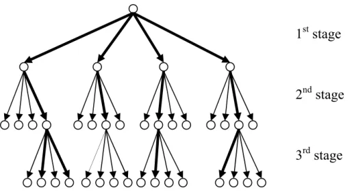
Based on (3.6), we can span a tree-like structure with depth NT, as shown in Fig.

(3.1). The process starts from the last element of x, i.e., xi, i = NT, because from

equation (3.6) we have yNT = rNT,NTxNT + nNT, where ri,i is the (i, i)th element of R,

suggesting that it has no interference from the other antennas. The algorithm calculates the metric for all possible values of xNT from the constellation set of size C using [13]

| ˜yNT−i+1− RNT−i+1xˆi|

2 _(3.7)

where ˜yi is the ith element of ˜y, Ri is the ith row of R and ˆxi = [ˆxi+1, ˆxi+2, . . . , ˆxNT]

is the vector of estimated symbols of the specific survivor path. Only M branches with the smallest metrics are retained and the rest of the list is discharged. This procedure is applied to the nodes of the next level, and is repeated until a tree depth of NT is

reached, i = 1.

The general detection process is described in Table 3.1 [13].

3

stage

2

stage

1

stage

Figure 3.1: Tree structure of QRD-M (M = 4), NT = 3, NR= 3, with 4-QAM

modula-tion.

Step 1 : Perform QR-decomposition on the channel matrix H. Step 2 : Premultiply the received vector y with QH_.

Step 3 : For every retained node, extend all branches to C nodes. Step 4 : Calculate the branch metrics using equation (3.7).

Step 5 : Retain only M branches with the smallest metrics and delete the rest of the list.

Chapter 4

Particle-Swarm-Driven

Cross-Entropy MIMO Detector

4.1

The Cross-Entropy Method

In this section, we give a detailed description of the concepts used in the Particle-Swarm-Driven Cross-Entropy (PSD-CE) method. We consider a single time slot only; the extension to T time slots is straightforward. The PSD-CE method is a Monte Carlo based stochastic approach to solve

arg min

x∈ANT_M

k y − Hxk2_{. (4.1)}

As the name suggests, this method combines the ideas of both Particle Swarm Opti-mization (PSO) and the Cross-Entropy (CE) method. Let us first begin with the latter approach.

Assuming perfect channel knowledge at the receive end, we define the score function

S(x) = k y − Hxk2_{. (4.2)}

In this situation, the optimal importance distribution g∗_{(x) should be a peak at ˆx} M L,

i.e. g∗_{(x) = δ(x − ˆx}

M L). Since we do not know g∗(x), we want to find the parameter

cross-entropy, a convenient measure of distance between two distributions, e.g. g(x) and f (x), is defined as [14] D(g, f ) = Eglng(X) f (X) = Z g(x) ln g(x)dx − Z g(x) ln f (x)dx (4.3)

Thus, our goal becomes

arg max v ·Z g∗(x) ln f (x; v)dx ¸ , (4.4)

where {f ( · ; v)} is a family of importance distributions on ANT

M . To solve the above

problem, we first use another distribution g0_{(x; w) to replace g}∗_{(x), where}

g∗_{(x; w) =} f (x; w) I{S(x) ≤ γ}

c (4.5)

S(x) = ky − Hxk2_{, I{ ·} is an indicator function and c is a constant for normalization.}

Notice that if f (ˆx; w) 6= 0 and γ = S(ˆx), g0_{(x; w) = g}∗_{(x). Let γ be the smallest}

value such that, under the distribution f (x; w), Pw({S(x) ≤ γ}) ≥ ρ, where ρ is a

predetermined parameter.

To find the smallest γ such that Pw({S(x) ≤ γ}) ≥ ρ can be done using the Monte

Carlo method. First draw U random samples, x1, . . . , xU, from f (x; u) and evaluate

their scores by S(x) respectively. Let γ be the dρUeth smallest score among all scores, then Pw({S(x) ≤ γ}) ≈ 1 U U X i=1 I{S(xi) ≤ γ} = dρUe U ≥ ρ (4.6)

Substitute g0_{(x; w) into (4.4), we obtain}

arg max v ·Z f (x; w)I{S(x) ≤ γ} c ln f (x; v)dx ¸ (4.7) By using the U random samples drawn from f (x; w) to estimate (4.7),

arg max v 1 U U X i=1 I{S(xi) ≤ γ} ln f (xi; v) (4.8)

we can obtain ˆv by solving 1 U U X i=1 I{S(xi) ≤ γ} ∂ ∂vln f (xi; v) = 0 (4.9)

Since the initial guess f (x; w) may not be a well-approximated g∗_{(x), we use f (x; ˆv) to}

approximate g∗_{(x) again. The above process is repeated to estimate another ˆv}0 _{and γ}0_.

In fact, we will iteratively estimate the parameter v(k)_{, γ}(k) _{and approximate the g}∗_(x)

by f (x; v(k)_{), where k is the iteration index. It is shown in [15] that the CE method}

converges, and if γ(k) _{converges to γ}∗ _{= S(ˆx) in the fixed number of iterations, we can}

get an exact solution.

4.2

Particle Swarm Optimization

In [11], it was shown that the performance of a CE-based MIMO detection algorithm exhibits an error floor in the high SNR region. Obviously, to remove the error floor and improve the detector performance with small sample size, other elements need to be included.

Particle Swarm Optimization (PSO) is an optimization technique inspired by birds-flocking. A swarm algorithm consists of a number of possible ‘particles’ (or samples) that move through the feasible solution space to explore the optimal solution. Every particle keeps a record of the position of its best performance, called the individual best position. The position of the best performance among all particles is the global best position. The PSO concept consists of changing the velocity of each particle towards its individual best position and the global best position, in every iteration. This concept is added into the previously mentioned algorithm. In every iteration, the best sample is recorded (relates to the individual best position), as well as the best sample over all the iterations (the global best position), and their influences are added when updating the new distribution. The evolutional concept acts as a driving force, pulling out the samples that have sunk into the undesirable local minima and pushing them towards the global minimum.

Step 1 : Initialize the distribution f(k)_(x

i) with uniform distribution

for i = 1, · · · , NT, respectively. Set k = 0.

Step 2 : Generate U samples xk

i,u from f(k)(xi) for u = 1, · · · , U and

construct the set {xk

u}Uu=1 where xku = [x1,uk , · · · , xki,u, · · · , xkNT,u]

T_.

Step 3 : Calculate the set of scores {S(xk

u)}Uu=1 according to

S(xk

u) = ||y − Hxku||2.

Step 4 : Find a γ(k) _{satisfying γ}(k) _{= arg min}

γ P (S(x) ≤ γ) ≥ ρ for x ∈ {x k u}Uu=1.

Then an elite set can be defined as {x|S(x) ≤ γ(k)_{, x ∈ {x}k u}Uu=1}.

Step 5 : Calculate the distribution of samples in the elite set:

f(k)

s (xi = a) =

P_U

u=1I{S(xku) ≤ γ(k)}I{xki,u = a}

P_U

u=1I{S(xku) ≤ γ(k)}

, (4.10)

where a ∈ AM for i = 1, · · · , NT.

Step 6 : Update the sample vector with the overall best score (from the 1st iteration to the kth iteration),xk

g(1), and the

best sample vector in the current iteration, xk p(1).

Step 7 : Update the distribution according to

f(k+1)_(x i = a) = α1fs(k)(xi = a) + α2f_g(1)(k)(xi = a) + α3f_p(1)(k)(xi = a) +¡1 −P3_i=1αi ¢ f(k)_(x i = a) (4.11) where α is the weighting factor and 0 ≤ α < 1.

Step 8 : Stop at iteration k = K if the pre-defined stopping criterion is met; otherwise, let k = k + 1 and go back to Step 2.

In (4.11), the weighting factors αi are smoothing factors that take the value between

0 and 1. The best values are found empirically, so that the PSD-CE method achieves a balance between exploration and exploitation. fg(1) and fp(1) are distributions given in

[11], based on xg(1) and xp(1), respectively.

4.3

Improving the PSD-CE Detector

Even with inclusion of a PSO element, the convergence speed of the PSD-CE method is still not fast enough. Thus, we propose a way to improve PSD-CE. In step 1 of the

algorithm above, the initial distribution, f(0)_(x

i), is set to be uniformly distributed. This

is the main reason of the slow convergence since the algorithm will need more iterations and samples to roam the entire solution space and converge at the best solution. A good initial distribution is crucial if a better performance or faster convergence is required.

Perform the Zero Forcing (ZF) method to find an initial solution, ˆxZF. The reason

we choose ZF is its low complexity. Although the ZF solution is usually not a very ‘good’ one, it still contains some information that can greatly improve the performance of the PSD-CE method.

The next problem is how to use the information drawn from ˆxZF. The ˆxZF gives a

rough idea about the whereabouts of the ˆxM Lso it would be a good decision to emphasize

the search more in that area. Given the jth element of ˆxZF, ˆxZF,j, where j = 1, . . . , NT,

the new initial distribution is designed as

f_j(0)(xi) = P_MDi k=1Dk (4.12) where xi ∈ AM, i = 1, . . . , M (4.13) and Di = 1 kˆxZF,j− xik2 . (4.14)

Since the summation of Di for i = 1, . . . , M does not add up to 1, the denominator of

(4.12) normalizes the probability distribution.

From (4.12), the probability of each entry xi in the constellation is given as the

reciprocal of the distance between ˆxZF,j and xi. In other words, the entries nearer to

ˆ

xZF,j are set to have larger probabilities, while those further have smaller probabilities.

Simulation results show that with this new initial distribution, the performance of the PSD-CE method has been greatly improved.

The additional computational complexity required to set the new initial distribution to all the elements of the constellation is (M − 1)NT additions and 17MNT

multiplica-tions ( here we assume that the complexity of division is equal to that of 8 mulplicamultiplica-tions), where M is the constellation size. The computational complexity needed to compute the Euclidean distance of a sample is NR(NT + 1) − 1 additions and (NT + 1)NR

mul-tiplications. Taking a 4 × 4 MIMO system with 16-QAM for example, the new initial distribution requires 64 additions and 1088 multiplications, while calculating the Eu-clidean distance of one sample requires 19 additions and 20 multiplications. Changing the initial distribution is equivalent to adding about 55 samples only! Hence, this small additional complexity results in a great improvement in the performance, as can be seen in the simulation results in Chapter 7.

Chapter 5

Signal Detection With CSI

Uncertainty

5.1

Effects of Channel Estimation Error

In the previous sections, the channel state information is assumed to be perfectly known at the receiver. However, in practical situations, pilot symbols are often employed to estimate the channel. Due to the finite number of pilots and noise, channel estimation errors are prone to exist. Hence, minimization of the Euclidean distance criterion is no longer optimum. Consideration of the errors of channel estimation has to be included in the optimal criterion. In most of the studies up until today, systems with channel estimation errors are modeled as

ˆ

H = H + E (5.1)

where E is the channel estimation error. However, according to the least squares method [25], the estimated channel should be orthogonal to the estimate errors. Hence, according to least squares, the channel should be modeled as

H = ˆH + E (5.2)

Under this assumption, we will derive the optimal criterion for the system in the presence of channel estimation errors.

Theorem 5.1.1. [27] Denote z1 and z2 circularly symmetric complex Gaussian random

vectors with zero means and full-rand covariance matrices Σij , E[ziz†j]. Then,

condi-tionally on z2, z1 is circularly symmetric complex Gaussian with mean Σ12Σ−122z2 and

covariance matrix Σ11− Σ12Σ−122Σ21.

We want to compute p(Y| ˆH, X), and we know that

p(Y| ˆH, X) =

NR

Y

i=1

p(Yi|X, ˆHi). (5.3)

Let z1 = Yi†= X†H†i+ Z†i = X†( ˆHi+ Ei)†+ Z†i and z2 = ˆH†i, then apply Theorem 5.1.1

to get Σ11 = X†X + σz2IT (5.4) Σ12 = X† ¡ INT − σ 2 eINT ¢ (5.5) Σ22 = INT − σ 2 eINT (5.6) Therefore, p(Y_i†|X, ˆH†

i) is circularly symmetric complex Gaussian distributed with

mean = X†_Hˆ†

i (5.7)

and

covariance matrix = σ_z2IT + σ2eX†X (5.8)

Finally, be multiplying p(Yi|X, ˆHi) from i = 1, . . . , NR as in (5.3), we obtain

p (Y| X, ˆH) = exp ½ tr ½ − ³ Y − ˆHX´ £σ2 zIT + σe2XHX ¤₋₁³ Y − ˆHX ´_H¾¾ det {π [σ2 zIT + σ2eXHX]}NR (5.9) Take the logarithm of (5.9) and drop the constant terms to achieve

ˆ XM L = arg minX NRln © det©σ2 zIT + σ2eXHX ªª + tr ½³ Y − ˆHX´ £σ_z2IT + σe2XHX ¤₋₁³ Y − ˆHX ´_H¾ (5.10) Note that with perfect CSI, P EP/σz2 → ∞, σe2 → 0, we will get the original metric, i.e.

5.2

QRD-M detection with imperfect CSI

Consider the case of one time slot only (generalization to T time slots is straightforward), equation (5.10) will simplify to

ˆ xM L = arg min x∈ANT_M " NRln ¡ σ_z2+ σ2_ekxk2¢+ ky − ˆHxk 2 (σ2 n+ σe2kxk2) # . (5.11)

In the QRD-M algorithm, we start the detection from the last layer, i.e., i = NT.

This is viable because R is an upper-triangular matrix hence the last element of the vector ˜y can be expressed as

˜

yNT = rNT,NTxNT + ˜nNT (5.12)

where ri,j is the (i, j)th element of R. ˜yNT does not contain interference from other

antennas, so no information of the elements from the upper layers are needed. When detecting upper layers, only the elements of the previously extended paths are used.

However, in (5.11), the term kxk2 _{in both the logarithm and denominator of the}

fraction causes a problem when we want to apply QRD-M under imperfect channel state information. This is because information of the elements of all the other layers will be needed at every detection layer.

In this thesis, we provide a way to solve this problem. Observe that the QR-decomposition can be performed on ˆH, i.e., ˆH = ˆQ ˆR. Keeping in mind that ˆQ is a unitary matrix and ˆR is an upper-triangular matrix, the term ky − ˆHxk2 _{can still be}

expanded into a tree structure.

ky − ˆHxk2 _{= ky − ˆQ ˆRxk}2

= k ˆQH_{y − ˆRxk}2 (5.13)

As the exact metric for a node cannot be obtained, we modify the optimization criterion in (5.11) by using a lower bound of the exact one.

Denote the metric to be minimized by Ξ(x), i.e. Ξ(x) = NRln(σ2n+ σ2Ekxk2) +

ky − ˆHxk2

(σ2

n+ σE2kxk2)

Suppose now we are at the ith detection layer, and ˆxi = [ˆxi, ˆxi+1, . . . , ˆxNT]

T_{, i =}

1, . . . , NT, are the estimated symbols in the current and previous layers of the path

in consideration. The lower bound for the metric in equation (5.14) in the ith detection layer is given as LB(Ξ(ˆxi)) = N ln(σn2 + σE2(kˆxik2+ (i − 1)Amin)) + ky − µ(ˆxi)k2 (σ2 n+ σ2E(kˆxik2+ (i − 1)Amax)) (5.15) where Amin and Amaxare the smallest power and the largest power of the symbol vectors

among the constellation alphabets, taking 16-QAM for example, Amin = 2 and Amax =

18. µ(ˆxi) is the multiplication of the corresponding ˆR and ˆxi. Think of equation (5.15)

as equation (5.14) under the best conditions in every detection layer.

The new QRD-M based detector begins from the first detection layer, i = NT. The

metrics for all possible values of ˆxi are calculated with equation (5.15). Only M nodes

with the smallest metrics are kept, and the rest of the list is discarded. The same steps are applied to the nodes of the next layer, and is done iteratively until i = 1. Finally, the path with the smallest metric is the estimated signal vector.

Chapter 6

Space Time Code

6.1

Background

In wireless communication systems with multiple antennas, we use space time codes (STC) to improve the transmission reliability, obtaining both diversity and coding gains. STC is based on joint encoding across space and time domains. STCs transmit redundant copies of the data stream to the receiver through multiple transmit antennas (transmit diversity). The transmitted signals will traverse different environments with scattering, reflection, and so on, resulting in different copies of the data at the receiver end. Some of the copies are better than others, meaning that they are less faded and thus provide more reliable information. In fact, the receiver combines all copies of the received signal in an optimal way to extract as much information from each of them as possible.

6.2

Alamouti Space-Time Block Code

In this section, we introduce the Alamouti space-time block code [19]. It is a simple orthogonal space-time block code with a maximum-likelihood decoding algorithm detec-tor. It is shown in [19] that with 2 transmit antennas, the scheme provides a diversity order of 2NR.

Alamouti. The Alamouti codeword is given by C = · s1 −s∗2 s2 s∗1 ¸ (6.1) In the case of BPSK, s1, s2 ∈ {−1, 1}. This scheme requires two signaling periods to

convey a pair of symbols s1 and s2. During the first time slot, the symbols s1 and s2 are

simultaneously transmitted from the first and second transmit antennas, respectively; then, in the next time slot, −s∗

2 and s∗1 are transmitted from the respective transmit

antennas.

The received signal matrix will be · y1,1 y1,2 y2,1 y2,2 ¸ = · h1,1 h1,2 h2,1 h2,2 ¸ · s1 −s∗2 s2 s∗1 ¸ + Z (6.2) where y1,1 = h1,1s1+ h1,2s2+ z1,1 y1,2 = h1,2s∗1− h1,1s∗2 + z1,2 y2,1 = h2,1s1+ h2,2s2+ z2,1 y2,2 = h2,2s∗1− h2,1s∗2 + z2,2

For operation convenience, we rewrite (6.2) as     y1,1 y∗ 1,2 y2,1 y∗ 2,2     =     h1,1 h1,2 h∗ 1,2 −h∗1,1 h2,1 h2,2 h∗ 2,2 −h∗2,1     · s1 s2 ¸ + Z0 _(6.3)

where it can be written with the more common notation

Yequi= HequiXequi+ Z0 (6.4)

Under the circumstances that the channel H is perfectly known at the receiver, the maximum likelihood (ML) detector can be derived to be

    h1,1 h1,2 h∗ 1,2 −h∗1,1 h2,1 h2,2 h∗ 2,2 −h∗2,1     †    y1,1 y∗ 1,2 y2,1 y∗ 2,2     = · hs 0 0 hs ¸ · s1 s2 ¸ +     h1,1 h1,2 h∗ 1,2 −h∗1,1 h2,1 h2,2 h∗ 2,2 −h∗2,1     † Z0 _(6.5)

where hs = |h1,1|2 + |h1,2|2+ |h2,1|2 + |h2,2|2. Note that this is also a zero-forcing (ZF)

detector, hence one of the many advantages of Alamouti coding is its easy decoding. It is interesting that when employing Alamouti codes with any constant envelope modulation, such as phase shift keying (PSK), the mismatched detector is exactly (6.5). The mismatched detector is expressed as

arg min

X

° °

°Yequi− ˆHequiXequi

° ° °2 = arg min X ³

Yequi− ˆHequiXequi

´_∗³

Yequi− ˆHequiXequi

´ (6.6) = arg min X Y ∗ equiYequi+ ³ XequiHˆequi ´_∗ ˆ

HequiXequi− 2Re

£ Y∗

equi(HequiXequi)

¤

Since Y∗

equiYequi is a constant term, when trying to find the argument that minimizes a

function, it can be omitted. The second term of the equation can be calculated as ³

XequiHˆequi

´_∗ ˆ

HequiXequi = X∗equiHˆ∗equiHˆequiXequi

= hsX∗

equiXequi (6.7)

= c I

where c is a constant, therefore, the second term in (6.6) can also be ignored. That leaves us with the last term in the equation. Denote XZF the solution found using the

ZF method, i.e. XZF = H∗equiYequi.

arg min

X −2Re

£

Y_equi∗ (HequiXequi)

¤ = arg max X Re £¡ H∗_equiYequi ¢_∗ Xequi ¤ = arg max X Re [X ∗ ZFXequi] (6.8)

Take QPSK symbols for example, Re£x∗_{ZF, i}xequi, i

¤

= Re[x∗_{ZF, i}]Re[xequi, i] + Im[x∗ZF, i]Im[xequi, i], i = 1, . . . , NT (6.9)

same is for the multiplication of the imaginary parts. We get the following equations: If Re[xZF, i] = Re[x∗ZF, i] > 0, Re[xequi, i] = 1 (6.10)

If Re[xZF, i] = Re[x∗ZF, i] < 0, Re[xequi, i] = −1 (6.11)

If Im[xZF, i] = −Im[x∗ZF, i] > 0, Im[xequi, i] = 1 (6.12)

If Im[xZF, i] = −Im[x∗ZF, i] < 0, Im[xequi, i] = −1 (6.13)

The above equations are exactly the ZF solutions! Thus, it is proved that when us-ing the Alamouti code with QPSK (and can be generalized to any constant envelope modulations), the mismatched detector is equivalent to the ML detector.

However, when the modulation does not have a constant envelope, such as 16−QAM, the mismatched detector of (6.5) is no longer optimal. In such cases, the ML decoding criterion is still given by (5.10).

6.3

Hamming based Space-Time Block Code

Richard Hamming proposed an error-correcting code that could correct a 1-bit error and detect 2-bit errors. This code, a binary linear error-correcting code, is named Hamming code [24] after its inventor. Let n be the length of the codeword, and k be the length of data bit, then it is apparent that n − k redundant bits are used for error checking. This is often referred to as the (n, k) code.

Denote the k × n matrix G the generator matrix of a linear (n, k) code and let H denote the (n − k) × n parity check matrix. G and H for linear block codes must satisfy

HGH _{= 0. (6.14)}

For Hamming code, to encode a k-bit data u, the corresponding n-bit codeword x can be obtained by

x = uG (6.15)

In this thesis, we consider the Hamming based space-time block code. The rationality behind choosing the Hamming based space-time block code is mentioned in [20].

The generating Hamming based space-time block code composed of two steps. First, the Hamming codeword is generated. Then, the codeword is multiplexed into two streams. The performance of Hamming based space-time block code depends on the multiplexing scheme and the optimal multiplexing scheme can be found through simu-lations.

Specifically, we consider a (8,4) binary Hamming based space-time block code. The generator matrix of (8,4) binary Hamming code is

G =     1 1 1 0 0 0 0 1 1 0 0 1 1 0 0 1 0 1 0 1 0 1 0 1 1 1 0 1 0 0 1 0     (6.16)

After encoding the data into a 8-bit codeword, x = [x1, . . . , x8], we multiplex the 8

bits into two streams. A possible multiplexing scheme is to fill in the first row and then the second row. Hence, the generated codeword is

X = · x1 x2 x3 x4 x5 x6 x7 x8 ¸ (6.17) However, we can also fill in the column first and the generated codeword is

X = · x1 x3 x5 x7 x2 x4 x6 x8 ¸ (6.18) The performance of these two multiplexing schemes and related comparison will be provided in Chapter ??.

Chapter 7

Simulation Results

This chapter is divided into two parts: In the first part, we present computer-simulated performance some conventional MIMO detectors as well as the PSDCE and the modified PSDCE detectors for a system with NT = 4 transmit antennas, NR = 4 receive

antennas and perfect CSI. In the second part, simulation results for the performance of detectors with modified ML criterion based on the nonzero channel estimation error are presented. We consider spatial multiplexing, Alamouti-coded and Hamming-coded MIMO systems.

7.1

Performance Comparison with Perfect CSI

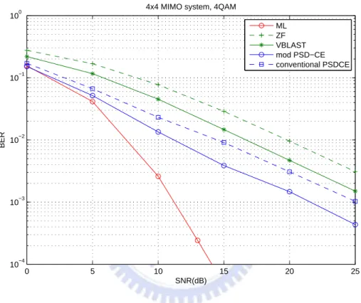
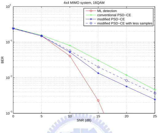
In Fig. 7.1, the BER performance comparison of some known detectors, such as ZF, V-BLAST, PSD-CE and modified PSD-CE, is shown. In this simulation, we generated 60 samples in every iteration for only 3 iterations, for both the PSD-CE detector and the modified PSD-CE detector using 4-QAM. We can see that the performance of the conventional PSD-CE is better than that of ZF and V-BLAST. It is also shown that the performance is further improved by the modified PSD-CE detector. Comparison between the BER performance of the conventional PSD-CE and the modified PSD-CE with 16-QAM is shown in Fig. 7.2. The solid lines are performances of the cases that run 5 iterations, and in every iteration 500 samples are generated. The proposed algorithm outperforms the conventional method by more than 5dB at BER= 10−2_{. The dotted line}

shows the performance of the modified PSD-CE with only 3 iterations, also generating 500 samples in each iteration. We can see that the performance of the modified PSD-CE even outperforms the conventional PSD-CE with a larger sample size! Therefore, it is obvious that the modified PSD-CE improves the performance, as well as decreases the complexity of the original PSD-CE method.

0 5 10 15 20 25 10−4 10−3 10−2 10−1 100 SNR(dB) BER

4x4 MIMO system, 4QAM

ML ZF VBLAST mod PSD−CE conventional PSDCE

Figure 7.1: Comparison of the BER performance of the modified PSD-CE detector (3 iterations and 60 samples/iteration) and other known detectors in a MIMO system with

0 5 10 15 20 25 10−3 10−2 10−1 100 SNR (dB) BER

4x4 MIMO system, 16QAM ML detection conventional PSD−CE modified PSD−CE

modified PSD−CE with less samples

Figure 7.2: Comparison of the BER performance of the conventional PSD-CE detector and the modified PSD-CE in a MIMO system with NT = NR = 4 using 16-QAM.

solid line : 5 iterations and 500 samples/iteration; dashed line : 3iterations and 500 samples/iteration.

7.2

Performance in the Presence of CSI Error

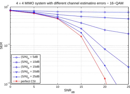
In this part of the simulations, we examine the influence of a system in the absence of perfect CSI at the receiver. Consider a MIMO system with NT = NR= 4 and 16-QAM

modulation. Figure 7.3 shows the frame error rate (FER) versus SNR in dB for different values of (S/N)P , P EP/σz2 with the mismatched metric, (2.19).

0 5 10 15 20 25 10−2 10−1 100 SNR_dB SER

4 × 4 MIMO system with different channel estimatino errors − 16−QAM

(S/N) P = 5dB (S/N)_P = 10dB (S/N) P = 15dB (S/N) P = 20dB (S/N) P = 25dB perfect CSI

Figure 7.3: Effect of channel estimation errors on the system performance.

7.2.1

Spatial multiplexing system

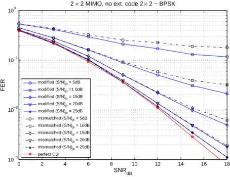
In this section, we consider the performance of spatial multiplexing (SM) system which uses two transmit antennas to transmit two independent data streams. For a 2 × 2 MIMO system, instead of a NR× 1 vector, let X be a NT × T matrix. Figures 7.4

and 7.5show the performances of T = 2 and 4 using the modified ML detector (5.10), respectively. The rate-2 code here implies that there is no actual ‘coding’, as it does not provide error correcting or detecting functions.

0 2 4 6 8 10 12 14 16 18 10−3 10−2 10−1 100 SNR dB FER

2 × 2 MIMO, no ext. code 2 × 2 − BPSK

modified (S/N) P = 5dB modified (S/N) P =1 0dB modified (S/N)_P = 15dB modified (S/N)_P = 20dB modified (S/N) P = 25dB mismatched (S/N) P = 5dB mismatched (S/N)_P = 10dB mismatched (S/N)_P = 15dB mismatched (S/N)_P = 20dB mismatched (S/N) P = 25dB perfect CSI

Figure 7.4: Effect of channel estimation errors on a 2 × 2 MIMO with T = 2 using BPSK. 0 2 4 6 8 10 12 14 16 18 20 10−4 10−3 10−2 10−1 100 SNR dB FER

2 × 2 MIMO, no ext. coding 2 × 4 − BPSK

modified (S/N) P = 5dB modified (S/N)_P = 10dB modified (S/N)_P = 15dB modified (S/N) P = 20dB modified (S/N) P = 25dB mismatched (S/N) P = 5dB mismatched (S/N) P = 10dB mismatched (S/N)_P = 15dB mismatched (S/N) P = 20dB mismatched (S/N) P = 25dB perfect CSI

Figure 7.5: Effect of channel estimation errors on a 2 × 2 MIMO with T = 4 using BPSK.

0 2 4 6 8 10 12 14 16 18 20 10−5 10−4 10−3 10−2 10−1 100 SNR_dB FER

2 × 2 MIMO with PSD−CE, no ext. coding 2 × 2 − BPSK

mismatched (S/N) P=5dB mismatched (S/N) P=10dB mismatched (S/N) P=15dB mismatched (S/N) P=20dB modified (S/N) P=5dB modified (S/N) P=10dB modified (S/N) P=15dB modified (S/N) P=20dB perfect CSI

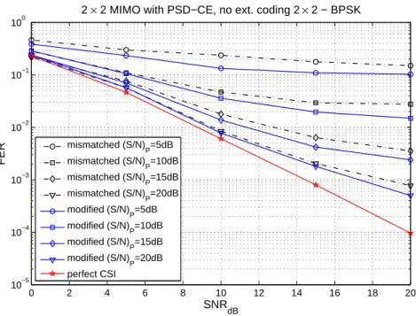
Figure 7.6: The use of PSDCE detector under channel estimation errors in a 2×2 MIMO with T = 2 using BPSK. 0 5 10 15 10−3 10−2 10−1 100 SNR dB FER

2 × 2 MIMO with PSDCE, no ext. coding 2 × 4 − BPSK

mismatched (S/N) P = 5dB mismatched (S/N) P = 10dB mismatched (S/N) P = 15dB mismatched (S/N) P = 20dB modified (S/N) P = 5dB modified (S/N) P = 10dB modified (S/N) P = 15dB modified (S/N) P = 20dB perfect CSI

Figure 7.7: The use of PSDCE detector under channel estimation errors in a 2×2 MIMO with T = 4 using BPSK.

7.2.2

Alamouti space-time coded system

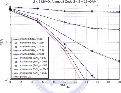
In this section, Alamouti code is employed in a 2 × 2 MIMO system using 16-QAM, i.e.

T = 2. Recall that the ML performance of the system using constant envelope

constella-tion is equal to that of the mismatched detector. Figure 7.8 shows comparison between the performances of the previously described system and the mismatched system. The gain is small but certain.

0 2 4 6 8 10 12 14 16 18 20 10−2 10−1 100 SNR dB FER

2 × 2 MIMO, Alamouti Code 2 × 2 − 16−QAM

modified (S/N) P = 5dB modified (S/N) P = 10dB modified (S/N) P = 15dB modified (S/N) P = 20dB modified (S/N) P = 25dB mismatched (S/N)_P = 5dB mismatched (S/N) P = 10dB mismatched (S/N) P = 15dB mismatched (S/N) P = 20dB mismatched (S/N) P = 25dB perfect CSI

Figure 7.8: Employing Alamouti code in a 2 × 2 systme with estimation errors with

T = 4 using 16-QAM.

7.2.3

Hamming coded system

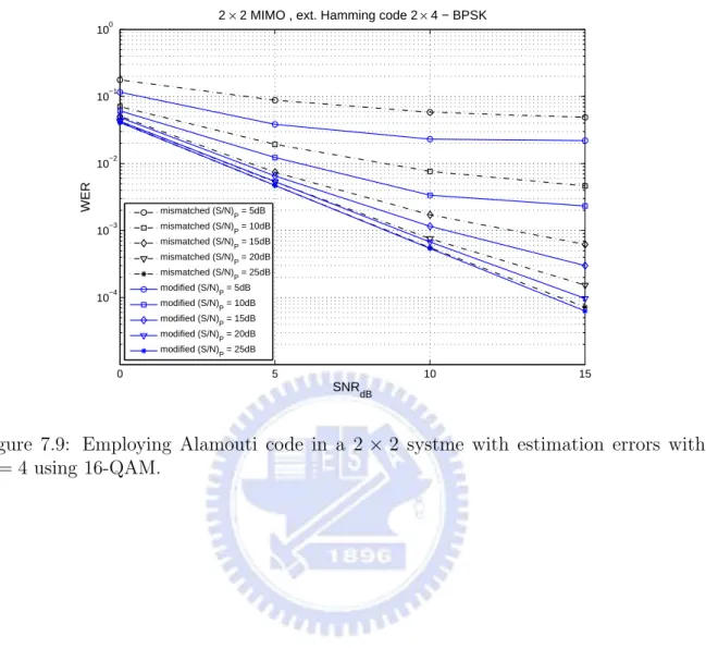
Here, we consider a space-time block code obtained by mapping a (8, 4) binary Hamming code to 2×4 BPSK codewords. The 8-bit Hamming codeword c = [c1, . . . , c8] is mapped

to the BPSK symbols like so

x = · x1 x2 x3 x4 x5 x6 x7 x8 ¸ (7.1) where xi = (−1)ci. In the first time slot, x1 and x5 are transmitted, then x2 and x6 are

7.9. 0 5 10 15 10−4 10−3 10−2 10−1 100 SNR_dB WER

2 × 2 MIMO , ext. Hamming code 2 × 4 − BPSK

mismatched (S/N)_P = 5dB mismatched (S/N) P = 10dB mismatched (S/N) P = 15dB mismatched (S/N) P = 20dB mismatched (S/N)_P = 25dB modified (S/N)_P = 5dB modified (S/N)_P = 10dB modified (S/N)_P = 15dB modified (S/N) P = 20dB modified (S/N) P = 25dB

Figure 7.9: Employing Alamouti code in a 2 × 2 systme with estimation errors with

Chapter 8

Conclusion

In this thesis, we investigate the optimum criterion of MIMO signal detection in the presence of channel estimation errors. Most existing studies on this subject assumed that the true channel matrix is independent of the associated error matrix. However, for least square or minimum mean square error channel estimators, the orthogonal principle implies that the channel estimator should be uncorrelated with the estimation error. Therefore, it is more appropriate to use such an assumption accordingly.

Although the optimal (ML)@detector can be derived, its high complexity makes it infeasible in practice. To overcomes this difficulty, we consider two sub-optimal detector structures that take imperfect CSI into account. The first suboptimal detector, referred to as Particle-Swarm-Driven Cross-Entropy (PSD-CE) detector, is a stochastic search based detection scheme. Its performance depends on the setting of the initial distribution and uniform distribution is often used for lack of a priori information. We propose a method to obtain the initial distribution which then leads to performance and complexity improvements. The other suboptimal detector is the modified QRD-M detector.

Since our design criterion is no longer equivalent to the minimum Euclidean distance criterion, the original QRD-M method cannot be used directly. We propose a low-complexity QRD-M detection method, using a new decoding metric which is derived from our assumption on the uncorrelatedness between the estimated channel matrix and the estimation error matrix. Finally, we extend our study to space-time block

coded MIMO systems and examine their performance using the new decoding metric. In all cases under investigation, we show by computer simulated numerical exam-ples that the proposed decoding metric does offer performance improvement over that achieved by using conventional metric that does not consider the imperfect CSI effect.

Bibliography

[1] D. Tse and P. Viswanath, Fundamentals of Wireless Communication, Cambridge University Press, 2005.

[2] E. Biglieri, R. Calderbank, A. Constantinides, A. Goldsmith, A. Paulraj and H. V. Poor, MIMO Wireless Communications, Cambridge University Press, 2007.

[3] I. Telatar, “Capacity of multiple antenna Gaussian channels,” Eur. Trans.

Telecom-mun., vol. 10, no. 6, pp. 585-595, Nov/Dec, 1999.

[4] R. Xu, F.C.M. Lau, “Performance analysis for MIMO systems using zero forcing detector over fading channels,” IEE Proc. Commun., Vol. 153, No. 1, February 2006. [5] G. H. Golub and C. F. Van Loan, Matrix Computations, Johns Hopkins University

Press, Baltimore, MD, 1983.

[6] P. W. Wolniansky, G. J. Foschini, G. D. Golden and R. A. Valenzuela, “V-BLAST: An architecture for realizing very high data rates over the rich-scattering wire-less channel,” Proc. of IEEE Int. Symposium on Signals, Systems and Electronics

(ISSSE’98), Pisa, Italy, Sep. 1998.

[7] R. Narasimhan, “Error propagation analysis of VVBLAST with channel estimation errors,” IEEE Trans. Commun., vol. 53, no. 1, pp. 27-31, Jan. 2005.

[8] V.Tarokh, A.Naguib, N.Seshadri, and A.R.Calderbank, “Space-time codes for high data rate wireless communication: Performance criteria in the presence of channel

estimation errors, mobility, and multiple paths,” IEEE Trans. Commun., vol.47, no.2,pp.199-207,Feb.1999.

[9] P. Hoeher and F. Tufvesson, “Channel estimation with superimposed pilot sequence,” in Proc. IEEE GLOBECOM’99, vol. 4, pp. 2164-2166, 1999.

[10] M. Biguesh and A. B. Gershman, “Training based MIMO channel estimation: A study of estimator tradeoffs and optimal training signals,” IEEE Trans. Sig. Proc., vol.54, no.3, pp. 884-893, March 2006.

[11] C. L. Wang, Y. T. Lin and Y. T. Su, “Particle-Swarm-Driven Cross-Entropy Method for MIMO Signal Detection,” IEEE WCNC 2010.

[12] J.Yue, K.J.Kim, J.D.Gibson, and R.A.Iltis, “Channel Estimation and Data Detec-tion for MIMO-OFDM systems,” in Proc, GLOBECOM 2003, pp.581-585,2003. [13] Chin,W.H. “QRD based tree search data detection for MIMO communication

sys-tems”, 2005 IEEE 61st Vehicular Technology Conference, Spring 2005.

[14] R. Y. Rubinstein and D. P. Kroese, The Cross-Entropy Method, Springer, 2004. [15] L. Margolin, “On the convergence of the cross-entropy method”, Annals of

Opera-tions Research, vol. 134, no.1, pp. 201-214, 2005.

[16] J. Kennedy and R. C. Eberhart, “Particle swarm optimization”, Proc. of the IEEE

Int. Joint Conf. on Neural Networks, pp. 1942-1948, 1995.

[17] F. Heppner and U. Grenander, “A stochastic nonlinear model for coordinated bird flocks”, S. Krasner, editor, The Ubiquity of Chaos, AAAS Publications, Washington, DC, 1990.

[18] V. Tarokh, N. Sheshadri and A. R. Calderbank, “Space-time codes for high data rate wireless communications: Performance criteria and code construction,” IEEE

[19] S. M. Alamouti, “A Simple Transmit Diversity Technique for Wireless Communi-cations”, IEEE Journal on Select Areas in Commun., vol. 16, no. 8, Oct 1998. [20] G. Taricco and E. Biglieri, “Space-Time Decoding With Imperfect Channel

Esti-mation”, IEEE Trans. on Wireless Communications, vol. 4, no. 4, July 2005. [21] B. Kim and K. Choi, “A Very Low Complexity QRD-M Algorithm Based on

Lim-ited Tree Search for MIMO Systems”, 2008 IEEE 67th Vehicular Technology

Con-ference, Marina Bay, Singapore, pp. 1246-1250, May 2008.

[22] A. A. Farhoodi and M. Fazaelifar, “Sphere Detection in MIMO Communication Sys-tems with Imperfect Channel State Information,” Proceedings of the Communication

Networks and Services Research Conference, pp. 228-233, May 2008.

[23] C. E. Shannon, “A Mathematical Theory of Communication”, Bell System

Techni-cal Journal, pp. 379-423(Part 1); pp. 623-656(Part 2), July 1948.

[24] R. W. Hamming, “Error Detecting and Error Correcting Codes”, Bell System

Tech-nical Journal, pp. 147-161, April 1950.

[25] S. M. Kay, Fundamentals of Statistical Signal Processing : Estimation Theory. En-glewood Cliffs, NJ: Prentice-Hall, 1993, vol. I.

[26] O. Weikert, U. Z¨olzer, “Efficient MIMO channel estimation with optimal training sequences,” Proc. of 1st Workshop on Commercial MIMO-Components and-Systems

(CMCS 2007), Duisburg, Germany, Sep. 2007.

[27] M. Bilodeau and D. Brenner, Theory of Multivariate Statistics. New York: Springer, 1999.

作者簡歷

林玉婷

民國七十四年十二月二十三日出生。

從小因為父親工作的關係，全家搬到馬來西亞。

民國九十三年畢業於檳城台灣學校，擔任多次班長、風紀股長、衛生股長

等，永遠考前五名因為班上只有 5 人。

民國九十七年畢業於國立交通大學電信工程學系，一年級加入交大羽球校

隊，從此便愛上了羽球。經過苦練，四年級之後成為大專盃團體賽上場球

員及梅竹上場球員，多次代表學校比賽，感到無比光榮。

同年推甄進入國立交通大學電信工程研究所碩士班，師蘇育德博士，兩年

來學到了很多，對老師的感激無法言喻。

國九十九年十月獲得碩士學位。

Graduate Courses：