國 立 交 通 大 學
機械工程研究所
碩士論文
應用於 3D 音效之殘響器的合成與最佳化設計
Optimal Design and Synthesis of Reverberators
for Three-dimensional Audio
研 究 生 : 白淦元
指導教授 : 白明憲
應用於 3D 音效之殘響器的合成與最佳化設計
Optimal design and synthesis of reverberators
for Three-dimensional audio
研 究 生: 白淦元 Student: Ganyuan Bai
指導教授: 白明憲 Advisor: Mingsian Bai
國 立 交 通 大 學
機械工程研究所
碩 士 論 文
A thesis
Submitted to Institute of Mechanical Engineering
Collage of Engineering
National Chiao Tung University
In Partial Fulfillment of Requirements
for the Degree of Master of Science
in
Mechanical Engineering
June 2003
HsinChu, Taiwan, Republic of China
應用於 3D 音效之殘響器的合成與最佳化設計
研 究 生:白淦元 指導教授:白明憲
國立交通大學機械工程學系
摘要
殘響音效為 3D 音效中之一重要部份,早期的殘響音效主要是透過設計一些 無限脈衝響應(IIR)濾波器來產生,但使用這種方法在聆聽時會有金屬聲跟一些不 自然的聲音產生。而後由於電腦運算速度的提升,現在的殘響器大部分都是用已 量測的真實房間響應以有限脈衝響應(FIR)的型式結構對輸入音訊做摺積,使用 此種方法不但耗時且耗經費。 本論文主要在發展一套經過參數最佳化設計之人 工殘響器,為了兼顧到殘響器的音質和運算量的降低,我們結合兩種方法:以 FIR 為 基 礎 的 虛 音 源 法 (image-source method) 來 模 擬 空 間 的 初 期 反 射 (early reflection),以及以一系列的 IIR 濾波器來產生晚期混響(late reverberation)。 此 外,我們建立了一套智慧型使用者介面,能讓使用者選擇所要聆聽的房間效果, 利用模糊理論來估算各種不同房間對應系統所需要的參數,並可經由視窗上的響 應圖形得到此房間的特性。Optimal Design and Synthesis of Reverberators for
Three-dimensional Audio
Student: Ganyuan Bai Advisor: Mingsian Bai Department of Mechanical Engineering
National Chiao-Tung University 1001 Ta-Hsueh Road, Hsin-Chu 30050
Taiwan, Republic of China
Abstract
Reverberator is an important element in three-dimensional audio reproduction. The audio will be sounded more spaciousness when using a well designed reverberator. Improperly designed reverberators were implemented by using many IIR filters and sounds with metallic and ringing or other artifacts. Genetic algorithms (GA) are employed to optimize the parameters of reverberators with high sound quality. In view of the trade-off of complexity and performance, an artificial reverberator is designed to play input music with reverberation in real-time. The reverberator we proposed is combining FIR-based early reflection and IIR-based late reverberation. The complexity of computation for our system is between the FIR-based and IIR-based reverberators. Besides, we use the concept of fuzzy logic to develop an intelligent user interface. The system can determine all the system parameters according to user’s choice of room modes.
誌謝
時光飛逝,短短兩年的研究生生涯轉眼就過去了。首先感謝指導教授白明憲 博士的諄諄指導與教誨,使我順利完成學業與論文,在此致上最誠摯的謝意。而 老師指導學生時豐富的專業知識,嚴謹的治學態度以及代人處事方面,亦是身為 學生的我學習與景仰的典範。 在論文寫作上,感謝本系呂宗熙教授和林家瑞教授在百忙中撥冗閱讀並提出 寶貴的意見,使得本文的內容更趨完善與充實,在此本人至上無限的感激。 回顧這兩年的日子,承蒙同實驗室的博士班曾平順學長、歐昆應學長、嚴坤 龍學長、蘇富城學長、陳榮亮學長、李志中學長與林家鴻學長在研究與學業上的 適時指點,並有幸與林振邦、董志偉、廖哲偉、曹登傑同學互相切磋討論,每在 烏雲蔽空時,得以撥雲見日,獲益甚多。此外學弟何柏璋、周中權、曾文亮及林 建良在生活上的朝夕相處與砥礪磨練,都是我得以完成研究的一大助因,在此由 衷地感謝他們。 能有此刻,我也要感謝所有在精神上給我鼓舞支持的人,謝謝各位的幫忙與 鼓勵。最後僅以此篇論文,獻給我摯愛的雙親白達奎先生、郭玉馨女士,以及哥 哥白為仁。今天我能順利取得碩士學位,要感謝的人很多,上述名單恐有疏漏, 在此也一一致上我最深的謝意。TABLE OF CONTENTS
摘要………....I ABSTRACT……….II 誌謝……….III TABLE OF CONTENTS………...IV LIST OF TABLES………..VI LIST OF FIGURES………..VII 1 Introduction………12 Theory and Method of Artificial Reverberators………..…………...3
2.1 Reproduction of Responses……….3
2.1.1 Echo Density………..5
2.1.2 Modal Density………5
2.1.3 Reverberation Time………5
2.1.4 Energy Decay Curve (EDC) and Energy Decay Relief (EDR)……..6
2.1.5 Modeling Early Reflection……….7
2.1.6 Modeling Late Reverberation……….7
2.2 Filter Building Blocks……….8
2.2.1 Comb Filter………8
2.2.2 Allpass Filter………..8
2.2.3 Nested Allpass Filter………..9
2.3 Synthesis of Artificial Reverberators………10
2.3.1 Feedback Delay Networks (FDN) Reverberator………..10
2.3.2 Multi-tap Delays and Bai’s Reverberator……….11
2.3.3 The Image-Source Method………...12
2.3.4 Nested Allpass Filters and Comb Filters………..13
3.1 Optimization of Early Reflection………..15
3.2 Genetic Algorithm……….16
3.3 Optimization of Late Reverberation by Using Genetic Algorithm…………..17
4 Artificial Reverberators by Using Fast Convolvers………..19
4.1 Block Convolution………19
4.2 FFT Block Convolution……….21
4.3 Fast Perceptual Convolution……….22
5 Fuzzy User Interface for Reverberators……….23
5.1 Fuzzy Logic and Fuzzy Inference System………24
5.2 Fuzzy User Interface for Artificial Reverberators……….24
5.2.1 Fuzzification……….25
5.2.2 Rule Evaluation………26
5.2.3 Defuzzification……….28
5.3 Graphic User Interface………..28
6 Conclusions………...……29
Appendix………...…..31
A Karaoke Effects………...31
A.1 Delay Modulation Effects………...31
A.2 Flanger Effect……….31
A.3 Chorus Effect………..32
A.4 Vibrato Effect……….32
A.5 Pitch Shifter………32
A.6 Detune Effect………..33
Reference………...……..34
Tables………...…36
LIST OF TABLES
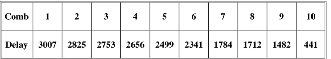
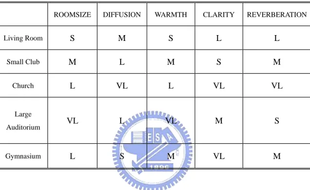
Table 1. The optimized delays of comb filter. ………...36 Table 2. The optimized delays and gains of nested allpass filters. ………36 Table 3. The relationship between five subjective indices and five room modes. 37
LIST OF FIGURES
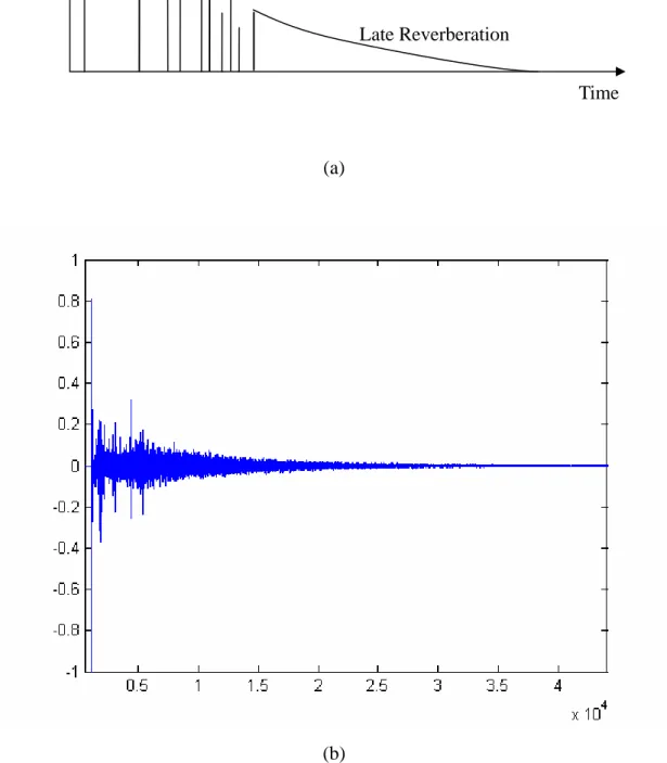
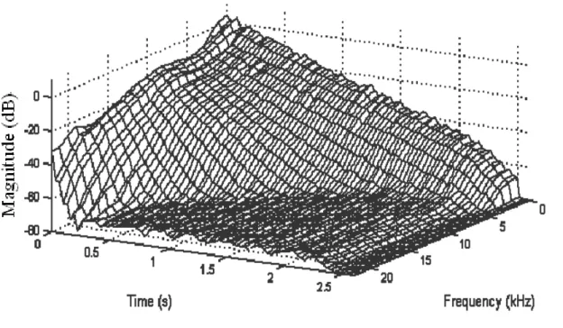
Figure 1. (a) Impulse response of St. John's Lutheran Church. (b) An ideal room response. ……….38 Figure 2. Energy decay relief (EDR) of a large hall. ……….39 Figure 3. Comb filter. (a) Block diagram. (b) Zero-pole plot. (c) Impulse response.
(d) Frequency response. ……….40 Figure 4. Allpass filter. (a) Block diagram. (b) Zero-pole plot. (c) Impulse
response. (d) Frequency response. ……….42 Figure 5. Nested allpass filter. (a) Block diagram (b) Impulse response of the
three-layer nested allpass filter with g1 =0.5, g2 =0.45, g3 =0.41 and delay lengths m1 =441, 533, 617.m2 = m3 = ………..44 Figure 6. (a) Stautner and Puckette’s four channel FDN. (b) FDN as general
specification of a reverberator containing N delays. ……….45 Figure 7. The results of two channel FDN. (a) The impulse response. (b) The
frequency response. ………....46 Figure 8. (a) Typical impulse response of the multiple delay effect. (b) The
direct-form FIR structure of the multi-tap delay. ………...47 Figure 9. The impulse response of the Bai’s Reverberator. ………...48 Figure 10. The impulse response by using image-source method with n=30, room
dimension = [10 8 3] and absorption coefficient is 0.8. ……….49 Figure 11. A regular pattern of image sources occurs in a rectangular room. …….50 Figure 12. Schroeder’s reverberator consisting of parallel comb filters and serial
Figure 13. (a) The structure of each comb filter, where the bp is the gain of absorbent lowpass filter and kp is the gain of comb filter. (b) The structure of ten parallel comb filters and three-layer nested allpass filters. (c) The structure of Nested allpass/comb reverberator with early reflection obtained via image-source method. ………...52 Figure 14. (a) The geometry of a rectangular room. (b) ELEF as calculated at
different position in room. ……….54 Figure 15. The flow chart of the optimization procedure for our scheme. ………..55 Figure 16. Absolute Threshold in quiet of human hearing. ……….56 Figure 17. The block diagram of fast perceptual convolution, where “PSP” is the
abbreviation of “perceptual sparse processing”. ………....57 Figure 18 The spectrum of the segmented impulse response recorded from St.
John's Lutheran Church. ………...….58 Figure 19 General model of fuzzy logic controller and decision making system. .59 Figure 20. The scheme of fuzzy user interface for artificial reverberator. ………..60 Figure 21. Gauss membership functions for the subjective indices. ………...61 Figure 22. Membership functions of the eight output parameters (a) Output
parameter Dim. (b) Output parameter Comb_d. (c) Output parameter Comb_g. (d) Output parameter Apd. (e) Output parameter Fc. (f) Output parameters Alpha,Ge, and Gr. ………....62 Figure 23. The first type-Mamdani’s minimum fuzzy implication rule, Rc. …....64 Figure 24. The fuzzy user interface of artificial reverberator with plot of impulse
response. ………...65 Figure 25. The fuzzy user interface of artificial reverberator with plot of frequency
Figure 26. The fuzzy user interf ce of artificial reverberator with plot of the EDC and T . ………...…...6760
Figure 27. The general structure of the Delay-Line Modulation. ………...68
Figure 28. Common Methods of Modulation. ……….69
Figure 29. The structure of a Flanger effect. ………...70
1 Introduction
Reverberation is a natural acoustical effect around our lives. Whatever sounds we listened in the world are immersed in somewhat reverberation effect. However the audio sound recording in a studio such as songs and music are dry (sounds without reverberation) that perceived not real enough and pleasurable. To add life to the dry recordings, through an instrument, called reverberator, to recreate such an echo effect that suits with the room which we want to listen. Besides, reverberator is a way to create the spaciousness and externalization effects, especially when headsets are used as the means of audio rendering. The reverberators will be realized by using many different artificial reverberation algorithms that will go into details in this thesis. Thanks to the pioneers of artificial reverberator, Schroeder and Moorer [1], numbers of reverberation algorithms developed for synthesizing room responses range from the allpass/comb filters network. Some of them are very relevant (Dattorro, Gardner, and Jot) offering different approaches to obtain a reverberation algorithm with some specific characteristics: natural sounding, absence of tonal coloration, high echo density, control of the reverberation time, etc. Those IIR (Infinite Impulse Response)-based reverberators, have the merit in low complexity, but are often difficult to eliminate unnatural resonances. First, a feedback delay network (FDN) model [2] presents in section 2.3.1, which can be seen as a generalized Schroeder’s parallel comb filter by using a diagonal feedback matrix. While this structure is capable to generate much higher echo densities than the parallel comb filters. As we implement a reverberator we construct a 2-input and 2-output model with diagonal feedback matrix. Another artificial reverberator we present in this thesis is the Bai’s reverberator in section 2.3.2 which was reformed from the idea of multi-tap delay effect. Instead of using comb filters in the reverberator, we recommend a time-vary recursive filter with exponential decay delay lengths. The advantage of using this
recursive filter is reducing the obvious peaks in frequency domain and making the “metallic” sounds disappear. However, the echoes we produce are too discrete and it leads to a grainy sound quality, particularly for impulsive input sounds. As a whole of these methods, whether simple or sophisticated, are based on the thesis of simplifying the algorithm and decrease the amount of computation. In order to determine an exact early reflection of the room with the given dimensions, we use the image source method [3] which constructs a 3D rectangular room and all virtual rooms around it. The details of using this method are shown in section 2.3.3. The third method of synthesis of reverberator we proposed is the nested allpass and comb filter reverberator. We recommend for using the nested allpass filters [4] that can increase the echo density with time and let the sounding effect more realistically in our reverberator. The details of this method will be described in section 2.3.4. The reverberator we recommend in this paper is combining the image source method for simulating the early reflections and nested allpass and comb filters for the late reverberation.
The optimum positions of the sound source and receiver that can produce the highest spaciousness will be presented in section 3.1. Allpass/comb filters network may be the most popular artificial reverberators. However, it generally takes quite an effort to adjust the parameters of the allpass/comb filters before an appropriate effect can be rendered. Concerning to this problem, we propose a way to optimize those parameters via the genetic algorithm (GA) that will present in section 3.2.
On the other hand, the FIR (Finite Impulse Response)-based reverberators, which convolve the input sequence with an impulse response modeling whatever rooms we want to listen. However, this method requires field measurements which needs quite large amount of processing power to carry on a computer and spends lots of money and time to measure the room response such as concert hall, church, and so on. In
chapter 4, a fast convolution technique, FFT (Fast Fourier Transform) block convolution, will be proposed for dealing infinity long input signal and long FIR room responses. On the other hand, the fast perceptual convolution [5], proposed by Chi-Min Liu, neglects the signals below the threshold in quiet and saves much computing complexity.
Chapter 5 proposes a way to determine the parameters of artificial reverberator that suite for the room we chosen via fuzzy user interface. It is a quicker solution for user to get the feeling of reverberation when they are listening music or songs. Besides, we build a graphic user interface with five particular environments. It can be executed by Matlab and play the sounds with reverberation effect but in off-line.
In this thesis, we propose a summary of most often used methods for artificial reverberator and some improvements and recommendations on designing a reverberator. Our ultimate goal is to design a less complexity and well performed reverberator that can play in real-time.
2 Theory and Methods of Artificial Reverberators
2.1 Reproduction of Room Responses Reverberation plays a vital role in 3D audio reproduction in that it creates a
realistic sensation of diffusiveness of sound field and spaciousness of the acoustic environment. To reproduce the reverberation of a room, we need to determine the room response first. Generally speaking, the room response can be divided into two distinct parts as shown in Fig. 1(a). The first part is composed of many discrete echoes of the original sound, called early reflections which present the geometric configuration of the room and the positions of the sound source and receiver. In general, this part of reverberation is in the region after the direct sound from 0 to about 80 msec. If the reflection delay is greater than about 80 msec, the reflection
will be perceived as a distinct echo of the direct sound. The second part is the late reverberation which composed of more dense echoes that decrease exponentially with time is related to the diffusion of sound and the background ambience. A real church’s impulse response and an ideal room response are presented in Fig. 1(b).
There are many methods for producing reverberation of a room, and we can classify them into two approaches. The first one, the physical approach, attempts to simulate exactly the propagation of sound from the source to the listener for a given room. The simplest and most direct method is to measure the room response in a real room, and then rendering the reverberation by convolution. When the room to be simulated doesn’t exist, we can attempt to predict its room response based on purely physical considerations, the geometry of the room, properties of all surfaces in the room, and the positions and directivities of the sources and receivers. However, this approach is computationally expensive and rather inflexible for real-time implement.
The second approach, called a perceptual approach, attempts to reproduce only the salient characteristics of reverberation. Without knowing the information of the room, we can construct a digital filter with N parameters that reproduces exactly N independent attributes reverberation, and then plug those parameter estimates into our reverberator. The method is generally much simpler constructed, more flexible and ideal than the physical approach.
This approach has many potential advantages:
The reverberation algorithm can be based on efficient infinite impulse response (IIR) filters which can be implemented without spending much computation. The reverberation algorithm can provide real-time control of all the perceptually
relevant parameters.
There are many important properties about the room response needed to be considered in the design of efficient reverberators and we will discuss them as follows:
2.1.1 Echo Density
In the time domain, the echo density of a room response was defined as the number of echoes reaching the listener per second.
3 4 ( ) 3 t ct N V π = , (1)
where N is the number of echoes, t is the time (in s), ct is the radius of the t
sphere (in m) centered at the listener, and V is the volume of the room (in m3). As differentiating with respect to t, we obtain that the density of echoes is proportional to the square of time:
3 2 4 t dN c t dt V π = . (2) 2.1.2 Modal Density
The normal modes of a room are the frequencies that are naturally amplified by the room. The number of normal modes N below frequency f is nearly f
independent of the room shape and is given as follows:
3 2 3 2 4 4 8 f V S L N f f f c c c π π = + + , (3)
where c is the speed of sound (in m/s), S is the area of all walls (in m2), and L is
the sum of all edge lengths of the room (in m). The modal density was defined as the number of modes per Hertz.
2 3 4 f dN V f df c π ≈ , (4)
Thus, the modal density of a room response grows proportionally to the square of the frequency.
The room effect is often characterized by its reverberation time (RT), a concept first established by Sabine in 1900. The reverberation time is proportional to the volume of the room and inversely proportional to the amount of sound absorption of the walls, floor and ceiling of the room. The Sabine’s empirical formula estimating the reverberation time lists as follows:
60 0.163 0.163 i i i V V T A a S ⋅ ⋅ = =
∑
, (5) where T is the time for the sound pressure to decay 60 dB, 60 V is the volume of the room (in m3), S and i a are the surface of a material employed in the room and the iassociated absorption coefficient, and the total absorption of materials is A . Since
most materials of surface in a room are more absorptive at high frequencies, the reverberation time of a room is also decreases as the frequency increases. The reverberation time is used for estimating the degree of sound absorption in a room.
2.1.4 Energy Decay Curve (EDC) and Energy Decay Relief (EDR)
The method to determine the reverberation time of a measured room is finding the time when the associated sound pressure attenuate 60 dB in the plot of the EDC, Schroeder proposed in 1965. He suggested integrating the impulse response of the room to get the room’s energy decay curve.
2 2 0 ( ) ( ) ( ) t h d EDC t h d τ τ τ τ ∞ ∞ =
∫
∫
, (6)where h(τ) is the impulse response of the room. Later, Jot proposed a variation of the EDC to help visualize the frequency dependent natural of reverberation called the energy decay relief EDR t
( )
,ω . The EDR represents the reverberation decay as afunction of time and frequency in a 3D plot. To compute it, we divide the impulse response into multiple frequency bands and compute Schroeder’s integral for each
band. An example, the EDR of a typical hall is shown in Fig. 2. 2.1.5 Modeling Early Reflection
The way to model early reflection of the reverberation has mentioned before, the physical approach. A room response from a source to a listener can be obtained by solving the wave equation also known as the Helmholtz equation. However, it can seldom be performed in an analytic form and is more complex in solving. Therefore, the solution must be approximated and there are three different approaches in computational modeling of room based on acoustics [3].
Wave-based methods Ray-based methods Statistical models
The ray-based methods, including the ray-tracing and the image-source methods, are the most often used modeling techniques. With the assumption of the wavelength of sound is small compared to the area of surfaces in the room and large compared to the roughness of surfaces, all phenomena due to the wave nature, such as diffraction and interference, are ignored. The image-source method examines the effects of an acoustic source in a room with corresponding sources located in image rooms with reflecting boundaries. Each of the infinite image sources will produce attenuated, filtered and delayed version of the original acoustic input. The total effects can be summed to produce a transfer function or a FIR filter.
2.1.6 Modeling Late Reverberation
There are two approaches to model late reverberation, the FIR-based and IIR-based methods. Implementing convolution using the direct form FIR filter is extremely inefficient when the filter size is large. Typical room responses are several seconds long, which at a 44.1 kHz sampling rate would translate to a huge number of points filter. One method to deal with the large size FIR filter is using an
algorithm based on the Fast Fourier transform (FFT) block convolution [6]. The second method is trying to model the late reverberation of a room based on some IIR-filters, comb and allpass filters, Schoroeder proposed first in the early 1960’s, or a mixture of them. The details of comb and allpass filters will be discussed in the next section.
2.2 Filter Building Blocks 2.2.1 Comb Filter
The block diagram of comb filter shown in Fig. 3 consists of a single delay line of m samples with a feedback loop containing an attenuation gaing . The z-
transform of the comb filter is given by:
( ) 1 m m z H z gz − − = − . (7)
Note that to achieve stability, g must be less than unity. The time response of
this filter is an exponentially decaying sequence of impulse spaced m samples apart. This is good for modeling reverberation because real room have a reverberation tail decaying somewhat exponentially. However, the echo density is really low, causing a “fluttering” sound on transient input. The pole-zero map of the comb filter shows that a delay line of m samples creates a total of m poles equally spaced inside the unit circle when it is stable. Half of the poles are located between 0 Hz and the Nyquist frequency / 2f = fs Hz, where f is the sampling frequency. That is why the s
frequency response has m distinct frequency peaks giving a “metallic” sound to the reverberation tail. We perceive this sound as being metallic due to hearing the few decaying tones that correspond to the peaks in the frequency response.
2.2.2 Allpass Filter
Because the poor performance of frequency response of a comb filter, Schroeder modified to provide a flat frequency response by mixing the input signal and the comb
filter output as shown in Fig. 4. The resulting filter is called an allpass filter because its frequency response has unit magnitude for all frequencies. The z-transform of the allpass filter is given by:
( ) 1 m m z g H z gz − − − = − . (8)
The poles of the allpass filter are thus the same as for the comb filter, but the allpass filter now has zeros at the conjugate reciprocal locations.
And the response of an all-pass filter sounds quite similar to the comb filter, tending to create a timbral coloration.
2.2.3 Nested Allpass Filter
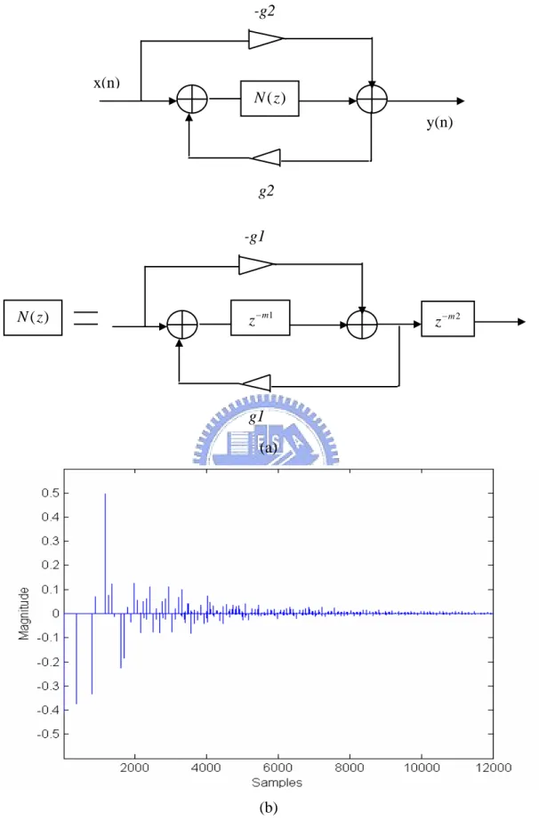
To achieve a more natural-sounding reverberation network, it would be desirable to combine the unit filters to produce a buildup of echoes, as it would occur in real rooms. One solution to produce more echoes is cascading multiple allpass filters which Schroeder had experimented with reverberators consisting of 5 allpass filters in series. Schroeder noted that these reverberators were indistinguishable from real rooms in terms of coloration, which may be true with stationary input signals, but other authors have found that series allpass filters are extremely susceptible to tonal coloration, especially with impulsive inputs. Gardner proposed reverberators based on a “nested” allpass filter, where the delay of an allpass filter is replaced by a series connection of a delay and another allpass filter. The block diagram and its impulse response are shown in Fig. 5(a), where the allpass delay is replaced with a system functionN z , which is allpass. Then the transfer function of this from is written: ( )
1 1 ( ) ( ) 1 ( ) N z g H z g N z − = − . (9) The advantage of using a nested allpass filter can be seen in the impulse response in Fig. 5(b). Echoes created by the inner allpass filter are recirculated to itself via the outer feedback path. Thus the echo density of a nested allpass filter increases
with time, as in real rooms.
2.3 Synthesis of Artificial Reverberators
2.3.1 Feedback Delay Networks (FDN) Reverberator
Gerzon [7] generalized the notion of unitary multichannel networks, which are
N-dimensional analogues of the all-pass filter. An N-input, N-output LTI system is
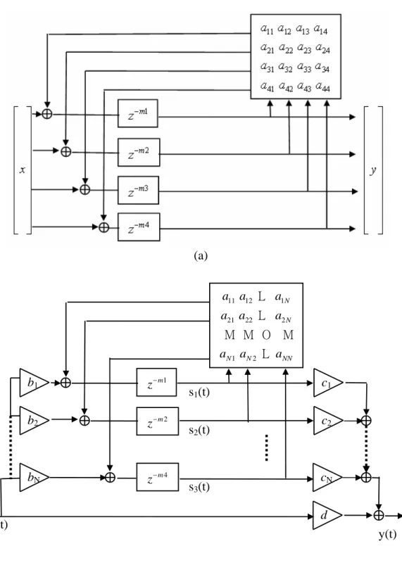
defined to unitary if it preserves the total energy of all possible input signals. Stautner and Puckette [8] then proposed a four channel general network based on four delay lines and a feedback matrix A, as shown in Fig. 6(a). In this matrix, each coefficient amncorresponds to the amount of signal coming out of delay line n sent to the input of delay line m. Gerzon found that the stability of this system is ensured if matrix A is the product of unitary matrix and an attenuated gain g with g <1.
To analyze the FDN system showed in Fig. 6(b), we derive the difference equations in the following:
1 ( ) ( ) ( ) N i i i y n c s n dx n = =
∑
+ , (10) , 1 ( ) ( ) ( ) N i i i j j i i s n m a s n b x n = + =∑
+ , (11) Using the z-transform, assuming zero initial conditions, we can rewrite Eqs. (10) and (11) in the frequency domain as( ) T ( ) ( )
Y z =c S z +dX z , (12) ( ) ( )[ ( ) ( )]
S z =D z AS z +bX z , (13) where sT(z)=[s1(z),Λ ,sN(z)] , ]bT =[b1,Λ ,bN and cT =[c1,Λ ,cN] . The diagonal matrix D(z)=diag(z−m1,z−m2,Λ ,z−mN)is called the “delay matrix”, and
N N j i
a
A=[ , ] × is called the “feedback matrix”.
Eliminating )s(z in Eqs. (12) and (13) gives the following system transfer function:
1 1 ( ) ( ) [ ( ) ] ( ) T y z H z c D z A b d x z − − = = − + . (14)
In simulation, we construct a 2-input, 2-output FDN reverberation. The feedback matrix A in our system is a unitary matrix ⎥
⎦ ⎤ ⎢ ⎣ ⎡ − = 1 1 1 1 2 1 U , and the
attenuation coefficients are mi
i
g =α , whereα =0.997,m1 =9 andm2 =6. To produce the effect of frequency dependent reverberation time, we add an absorbent filter that was proposed by Jot [9] in 1991. The absorbent filter method is to add a low-pass filter in each delay line for decaying the high frequency signals. The low-pass filter we used is a one-order filter with cut of frequency at 10 KHz. The result impulse and frequency response of the 2-channel FDN reverberator is shown in Fig. 7.
2.3.2 Multi-tap Delays and Bai’s Reverberator
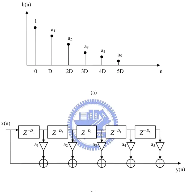
Multiple delayed [11] values of an input signal can be combined easily to produce multiple reflections of the input. This can be done by having multiple taps pointing to different previous inputs stored into the delay line, or by having separate memory buffers at different sizes where input samples are stored. The typical impulse response of the multiple delay effect is presented in Fig. 8 (a). The difference equation is a simple modification of the single delay case. For instance, the difference equation of a 5 delays multi-tap delay processing algorithm would perform as the following:
1 1 2 2 3 3 4 4 5 5
[ ] [ ] [ ] [ ] [ ] [ ] [ ]
y n =x n +a x n−D +a x n−D +a x n−D +a x n−D +a x n−D . (15) The multi-tap delay can be performed as the direct-form FIR structure that shown in Fig. 8(b). In order to add an infinite number of delays, the difference equation then becomes an IIR comb filter. As a result of some disadvantages of the comb filter, we develop the pattern of the Bai’s reverberator by using the concept of the delay modulation whose delay-line center is varying with time. The details of the delay
modulation effects will be mentioned in appendix.
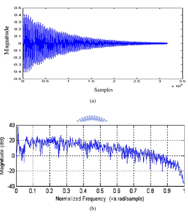
The bad performances, a noticeable and unpleasant sound likes a beating in a parallel wall back and forth, for the comb filter are owing to the poles in zero-pole domain and the peaks in frequency domain spaced equally. To solve this problem, we substitute the comb filter for a time-varying recursive IIR filter with an exponential decay delay length in our reverberation system. As the same reason of increasing the echo density and modal density for the Schroeder’s reverberator, we parallel multiple time-varying recursive IIR filters to increase the echo density. In practically, the structure of the Bai’s reverberator we constructed is one filter to
present the early reflection and series another one to present the late reverberation. The advantage of using this model is reducing the obvious peaks in frequency domain
and making the “metallic” sounds disappear. However, the echoes we produce are too discrete and it leads to a grainy sound quality, particularly for impulsive input sounds. The result via this scheme is shown in Fig. 9.
2.3.3 The Image-Source Method
The main mathematical approaches of modeling spatial sound fields are wave-based methods and ray-based methods. The wave-based methods are the more computationally demanding techniques such as the finite element method (FEM) and boundary element method (BEM). The techniques are suitable for simulation of low frequencies only. However, the ray-based methods, the ray-tracing and the image-source methods [12] [13], are based on geometrical room acoustics, in which the sound is supposed to act like rays. The basic distinction between the ray-tracing and the image-source methods is the way the reflection paths are typically calculated. There is an assumption of using the ray-based methods, that is, the wavelength of sound is small compared to the area of surfaces in the room and large compared to the roughness of surfaces. The image-source method finds all the paths, but the
computational requirements are such that in practice only a set of early reflections is computed. The maximum achievable order of reflections depends on the room geometry and available calculation capacity. The number of reflections calculated by this method for each reflection order in a rectangular room can be formulated as follows:
2
4 2
n
N = n + , (16)
where Nn is the number of sources of the nth order reflection. The total image point grows proportionally to the square of n. In image-source method, reflected paths from the real source are replaced by direct paths from reflected mirror images of the source. If the n is large enough, the impulse response of the sound source will abound with reflections. Figure 10 presents the impulse response by using image-source method with the 30 order reflection. Because of calculation capacity of the early reflection in our reverberator, we set the order of maximum reflection to 6 and there will be 376 sources with difference paths.
The evaluation of the impulse response of the enclosure is then made by recording the arrivals of the impulses from all the image sources in the lattice, these impulses having a strength equal to that of the real source and being emitted simultaneously with the real source. The room used for the calculations was rectangular with the same absorbing sidewalls, ceiling, and floor. Figure 11 presents a regular pattern of image source occurs in an ideal rectangular room.
2.3.4 Nested Allpass Filters and Comb Filters
Schroeder proposed a reverberator consisting of four parallel comb filters and two series all-pass filters, shown in Fig. 12. The purpose of using multiple parallel comb filters is to increase modal density and echo density, while using series allpass filters would increase echo density more effective.
As mentioned in section 2.1.1 and 2.1.2, the modal density and echo density, we can estimate how many comb filters would be needed by knowing how the modal density and echo density are in our system.
1 1 N f i i s D m F = =
∑
, (17) 1 N s t i i F D m = =∑
, (18) where Df is the modal density, Dtis the echo density,Fsis the sampling rate in our system, N is the number of comb filter we need and miis the thi comb filter delay
length.
Combining Eqs. (17) and (18), we can get the number of comb filters we need.
f t
N = D ⋅D . (19) As the basic concept of comb filter mentioned before in section 2.3.1, the reverberation time Trfor a comb filter is given by:
10 20 log ( )i 60 i r g m T T − = , (20)
where T is the sampling period. For a desired reverberation time, we can choose the delay length and the feedback gain to tradeoff modal density for echo density. From Eq. (20), the attenuation gains giof the comb filters are set to give a desired reverberation time Traccording to
3 / 10 i r i
m T T
g = − . (21) Based on those criterions mentioned above, we now propose a reverberator whose late reverberator consists of ten parallel comb filters and cascades three layers nested allpass filters [14] [15]. The absorbent filter we used here is a one-order low-pass filter with a coefficient α which is the ratio of the reverberation times at Nyquist frequency and zero frequency. While the early reflection of this
reverberator, using the image-source method to model a rectangular 3D virtual room with the scale we determined and the positions of source and receiver we given. The structure of the reverberator is shown in Fig. 13.
3 Optimal Design of Reverberators
To design a well listening reverberation system, the all parameters in the reverberator must be optimized. In this chapter, we will propose the genetic algorithm (GA) to deal with the nonlinear parameter optimization and to prevent from trapping into local minimum problems.
3.1 Optimization of Early Reflection
In this section, we introduce some objective measures that will permit judging the quality of hearing of the early reflection in a room. Many researches in room acoustics were finding a rating that emphasizes the effect of sound reflections coming from different directions on the sensation of spatial impression. The spatial impression is a consequence of the uniformity of the directional distribution of sound. The early lateral energy fraction (ELEF) [16], first proposed by Barron and Marshall, which evaluates the proportion of early lateral sound energy reaching a listener as compared to the total sound energy during the first 80 ms of the impulse response. This parameter has been found to be strongly correlated with the impression of spaciousness and is given by
80 2 5 80 2 0 ( ) ( ) ms L ms ms P t dt ELEF P t dt =
∫
∫
, (22)where P tL2( )=P t2( ) cosθ , θ being the angle between the incident pulse and the line normal to the median of the listener’s head, and P is sound pressure.
spaciousness S, which is defined by 80 2 5 80 2 2 0 ( ) 1 /100 ( ) ( ) ms L ms ms L p t dt ELEF S ELEF p t p t dt = ≈ − ⎡ − ⎤ ⎣ ⎦
∫
∫
. (23)In the part of constructing early reflection by using image-source method, the ELEF is the cost function and the input parameters are room size dimensions (length, width and height), and the position of sound source and receiver unit. The goal of our optimum here is to find the locations of source and receiver that will maximize the ELEF and produce the most spaciousness.
The room size dimensions are based on what kind of room we choose. In our simulation system, we define a medium rectangular room with its length, width and height are 15m, 8m, and 3m respectively. Figure 14(a) shows the geometry of the room we simulated, and the sound source is at (0.5, 0.5, 2). The plot of ELEF corresponding to the sound source is presented in Fig. 14(b). From the distribution of the value of ELEF, we can find that the spaciousness becomes larger as the receiver more away from the source in both x and y axes.
3.2 Genetic Algorithm
Genetic algorithm is a search algorithm based on the mechanics of natural selection, genetics and evolution. The main principle of GA is that it encodes input parameters of population strings into binary digits (1s and 0s) called chromosomes, which represent multiple points in the search space. The resolution of a parameter space is depended on the amount of bits per string and searching domain of the parameter. For instance, the parameter A isl encoded into a binary string of length
ll and the Resolution can be obtained as follow
, 2 1 l l U L l l A l A A R = − − (24)
where A and lU A are the upper and lower limits of the parameter lL A . l
The optimal solution can generally be found by within several generations. In each generation, three basic genetic operators, reproduction, crossover and mutation, are generated a new population and chromosomes of the population. In the reproduction process, the individual beings are survived according to their fitness value which determines the probability acted on genetic operators. The crossover process performs genes exchange between two chromosomes from the parents and it will occur when a random number between 0 and 1 is less than the crossover probability Pc. The mutation process prevents the population from becoming too
homogenous and leading to premature convergence at non-optimal result. Next, the natural selection process finds the best chromosome and reproduces it by substituting their population into a fitness function in that generation. From generation to generation, the optimal solution can be found. The GA procedure applied to our late reverberator design problem is detailed as follows.
3.3 Optimization of Late Reverberation by using Genetic Algorithm
In the parallel comb filters and nested allpass filters system for modeling late reverberation, the input parameters are comb filter delays, comb filter attenuation gain, allpass filter delays, allpass filter attenuation gains, and the low-pass filter coefficient α . It is less efficient and wasting time for searching the eighteen optimized coefficients by GA at one time. Based on the difference performances among those filters, we divide our system into four steps. The coefficients that we will optimize in the first step are the three delays and three gains of the three-layer nested allpass filters d and i gi (i=1, 2, 3). The upper and lower limits for the delays are defined as 1000 and 50 and for the gains are defined as 1 and 0.1. The goal of optimization in this step is to deal a high echo density Ed and a high impulse energy En. Therefore,
the fitness function F1( )θ1 is defined as follows
1( )1 d( )1 n( ),1
F θ =E θ +wE θ (25) where θ1=[ d d1 2 d3 g g1 2 g3] is the chromosome and w is the weighting between those two cost functions of Ed( ) and θ1 En( )θ1 .
In the second step, we want to optimize the ten delays of the parallel comb filters ( 1, 2 10)
i
c i= L . The upper limit here is set to 3528 samples (80ms), and the lower limit is 441 samples (10ms) for a middle size room. The objective is to find the best chromosome so that the echo density and the modal density M could reach highest d
simultaneously. By the way, we estimate the modal density by calculating the number of poles existed on pole-zero map. The fitness function F2(θ2) is defined as follows
2( )2 d( )2 d( ),2
F θ =E θ ×M θ (26) where θ2 =[ c c1 2 L c10]. In a comb filter, the model density will be decreasing when the echo density is increasing. For the reason of the trade-off between echo density and modal density, we use a multiplication here between those two parameters.
In the third step, we evaluate the gain of comb filters by a given constraint that is the reverberation time (T60) of room. When the value of the T60 has been evaluated from the room, we can search for the best gain of comb filter via GA. If the gain that we choose let the total T60 over the constraint, the step will not be stopped until it finds the proper one.
Finally in the fourth step, we get the impulse responses that created by the software of Cool Edit Pro.2.0 with the difference room modes, like church, living room or large auditorium and so on. In each room mode, we transform the impulse response into frequency domain and find the best chromosome of the parameter of α so that the frequency response curve approximates the desired one. The fitness
function is defined as
4 min( ( ) ˆ( ) ), t
F = P t −P t (27)
where ( )P t is the desired frequency response and P tµ( ) is the synthesized frequency response. The flow chart of the optimization procedure for our scheme is shown in figure 15.
There are forty populations formed randomly per parameter, and the each population contains eight chromosomes. The crossover rate and mutation rate are 0.85 and 0.008. After executing each step with 100 generations, the GA optimization procedures are conducted to find the best parameters to our late reverberation. The optimum parameters we determined are listed in Table 1 and Table 2.
4 Artificail Reverberators by Using Fast Convolvers
4.1 Block Convolution
FIR-based reverberators are implemented by convolution methods. The input signal that we processed is always infinity in length, and it needs to be segmented into several of block signals. There have been two approaches to deal with the FFT block convolution: overlap-and-save method and overlap-and-add method. The convolution between input signal x[n] and impulse response h[n] of length L is expressed as 1 0 [ ] [ ] [ ] [ ] [ ] L k y n x n h n x n k h k − = = ∗ =
∑
− . (28) The overlap-and-add method adopts non-overlapped input segments to calculate overlapped output segments. The overlapping occurs because the linear convolution of each segment with the impulse response is longer than the length of the segment. To extend the overlap-and-add approach to block convolution, let the input signals x[n]and impulse response h[n] are segmented as a sum of finite-length segments of length N; i.e., 0 [ ] r[ ] r x n x n rN ∞ = =
∑
− , (29) and 1 0 [ ] [ ] M s s h n h n sN − = =∑
− , (30) where M is the number of how many blocks of the impulse response except the least one that the length is small than N, i.e. M LN ⎡ ⎤ = ⎢ ⎥⎣ ⎦. [ ], 0 1 [ ] 0, otherwise r x n rN n N x n = ⎨⎧ + ≤ ≤ − ⎩ (31) and [ ], 0 1 [ ] 0, otherwise s h n sN n N h n = ⎨⎧ + ≤ ≤ − ⎩ (32) Substituting Eqs. (29) and (30) into Eqs. (28) yields
1 0 0 [ ] [ ] [ ] M r s r s y n x n rN h n sN ∞ − = = ⎧ ⎫ ⎧ ⎫ =⎨ − ⎬ ⎨∗ − ⎬ ⎩
∑
⎭ ⎩∑
⎭ (33) Because convolution is linear time-invariant, it follows that1 1 , 0 0 0 0 [ ] [ ] [ ] [ ] M M r s r s r s r s y n x n rN h n sN y n rN sN ∞ − ∞ − = = = = =
∑∑
− ∗ − =∑∑
− − (34) where yr s, [ ]n =x nr[ ]∗h ns[ ], for 0≤ ≤n 2N-1 (35) The overlap-and-save method implements the circular convolution or linear convolution of the impulse response with the overlapped inputs, and the resulting output segments are patched together to from the output. If an L-point sequence is circularly convolved with a P-point sequence (P < L), then the first (P-1) points of the result are incorrect. Therefore, we can divide x[n] into sections of length L so that each input section overlaps the preceding section by (P-1) points. That is, we define the sections as[ ] [ ( 1) 1], 0 -1
r
x n =x n+r L− + − +P P ≤ ≤n L (36) The circular convolution of each section with hs[n] is denoted as yr,sp[n] in which time
aliasing has occurred. 1 , 0 0 [ ] [ ( 1) 1] M r s r s y n y n r L P P ∞ − = = =
∑∑
− − + + − , (37) where , , [ ], 1 1 [ ] 0, otherwise r sp r s y n P n L y n = ⎨⎧ − ≤ ≤ − ⎩ . (38) This procedure is called the overlap-and-save method because the input segments overlap, so that each succeeding input section consists of (L-P+1) new points and (P -1) points saved from the previous section.The comparison between these two methods is discussed as follows. By using the overlap-and-add method, the overlap output samples must be added together and needed to define a larger buffer to store the output than the overlap-and-save method. However, using the overlap-and-save method, the correct output samples are less than using the overlap-and-add method and the more input blocks will be segmented. For the convenience of processing the output signals, we adopt the overlap-and-save method for the FFT block convolution.
4.2 FFT Block Convolution
In this section, we use the overlap-and-save method to implement the FFT block convolution by transforming each pair of small blocks to DFT domain and performing multiplications on DFT domain. Since the complexity of the specific sizes of DFT can be reduced form O(N2) to O(NlogN) by FFT algorithms, these algorithms can perform the convolution with significant speed improvement.
To estimate the complexity of FFT block convolution in our FIR-based reverberator, we set each impulse response block size to 4,096 samples and the input signal block size to 8,192 samples. The impulse response that we measured in a
church has 49,152 samples and be segmented to 12 blocks. First, we transfer each impulse block to FFT domain with 8,192 points and it needs
2
4096 log 4096=49,152multiplications and additions. The total complexity of computation with storing the FFT data of the segmented impulse response is 589,824 multiplications and additions. For transferring each block of input signal to FFT domain with 8,192 points needs 116,496 multiplications and additions. In the frequency domain, we multiply the impulse response and input signal and determine the summation of the 12 blocks impulse response. There are 12×8,192 complexity of multiplications and (12-1)×8,192 complexity of additions. To execute the inverse FFT with 8,192 samples, we need another 116,496 multiplications and additions. Thus, the total complexity of computation is 56.35 million multiply -accumulate per second (MMACS) for a stereo signal with 44.1k sampling rate.
4.3 Fast Perceptual Convolution
The fast perceptual convolution is the way to reduce the computational complexity required by FIR-based reverberators. However, the threshold in quiet is the threshold to characterize the minimum amount of energy needed in human hearing system in a noiseless environment. The main principle of the fast perceptual convolution is to reduce the multiplications needed in frequency domain below the threshold in quiet and can be integrated well with the FFT-based convolution methods. The segmented impulse response of the FIR filter becomes sparse and hence reduces the complexity.
One well known threshold is the one made by Painter and Spanias [17]. The output signal of each output block Y k will not be perceptible if the energy is r'[ ] lower than the threshold. The r’ here is distinguished from the r for the overlap-and-add method. That is
'[ ] [ ] r
Y k ≤Tq k , (39) and
Tq k[ ]=3.64( /1000)k −0.8−0.65e−0.6( /1000 3.3)k − 2 +10 ( /1000)−3 k 4, (40) where [ ]Tq k is the threshold in quiet for a frequency k (in dB). The plot of
threshold in quiet is presented in Fig. 16. Because each blocked output is the summation of the multiplication of the input blocked signal and segmented impulse response in frequency domain.
1 ' ' 0 [ ] [ ] [ ] M r r s s Y k X k H k − = =
∑
. (41) Substituting (38) to (40) leads to 1 ' 0 [ ] [ ] [ ] M r s s X k H k Tq k − = ≤∑
. (42) Because the maximum signal magnitude is set to 1, (41) can reduce to1 1 ' 0 0 [ ] [ ] [ ] [ ] M M r s s s s X k H k H k Tq k − − = = ≤ ≤
∑
∑
. (43) The sufficient condition for the above inequality on H ks[ ] isH ks[ ] Tq k[ ]
M
≤ . (44)
In other words, we can directly truncate the small values of H ks[ ] into zeros to
reduce the complexity according to (44). The block diagram of fast perceptual convolution is shown in Fig. 17, and the spectrum for all the segmented impulse responses is shown in Fig. 18. The higher frequency part will decay faster than lower frequency part.
5 Fuzzy User Interface For Reverberators
In this chapter, we utilize the concept of fuzzy logic [18] to determine the input variables of the artificial reverberator we proposed, and build a fuzzy control system
as a user interface.
5.1 Fuzzy Logic and Fuzzy Inference System
Fuzzy logic is a technology for developing sophisticated inference and human decision of reducing and explaining system complexity. A fuzzy inference system works with an input value, performs some calculations, and generates an output value. It includes a fuzzifier, a fuzzy rule base, and a defuzzifier. The typical architecture of a fuzzy inference system is shown in Fig. 19. In the fuzzifier, there are several types of membership function which transform input data into suitable linguistic values. The fuzzy rule base stores the empirical knowledge of the operation of the process of the domain experts. The defuzzifier is used to yield a nonfuzzy decision or output from an inferred fuzzy input.
5.2 Fuzzy User Interface for Artificial Reverberators
In order to realize our artificial reverberator without making a decision with many input parameters, we propose the scheme of using friendly user interface [19] via fuzzy inference. In Figure 20, we can see that the scheme of fuzzy user interface for artificial reverberator is composed of two stages. In the first stage, we summarize the five subjective indices to describe the reverberation impression such as
Room_size, Diffusion, Warmth, Clarity and Reverb. The relationship between those
subjective indices and what the room mode we chose is presented in Table. 3. In our system, we choose the five most familiar room modes, and they are Living Room, Small Club, Church, Large Auditorium and Gymnasium, respectively. In the second stage, we use the fuzzy control system to transform those five subjective indices into eight system parameters corresponding to the inputs of our artificial reverberator. The eight system parameters are Dim (room dimension), Comb_d (comb filter delay),
Comb_g (comb filter gain), Apd (allpass filter delay), Alpha (high frequency ratio), Fc
reverberation gain). We use common-sense fuzzy rules for the determination of quantization level. Fuzzy rules deal with room effect as fuzzy association (Ai, Bi) representing the linguistic rule “IF X is Ai, Then Y is Bi”.
5.2.1 Fuzzification
In the first stage of our fuzzy inference system, the R (room mode) is the only one fuzzy variable. If we choose the LR (Living room), SC (Small club), CH (Church), LA (Large auditorium), and GY (Gymnasium), the value of Room_mode is set to 0.2, 0.4, 0.6, 0.8, and 1.0 respectively. In each subjective index decision, four fuzzy membership functions, namely, S (small), M (medium), L (large), and V (very large) are assigned to their input. Gauss function is adopted here for the membership functions of those subjective indices shown in Fig. 21. The mathematical formula of Gauss membership function is represented as follows:
2 2 ( ) 2 gauss( , , ) x b a x a b e ⎡− − ⎤ ⎢ ⎥ ⎢ ⎥ ⎣ ⎦ = . (45) In the second stage of our fuzzy inference system, these five subjective indices are the fuzzy inputs and the eight system parameters are the fuzzy outputs. The
Room_size is the index for presenting how large the room that we chose is. The
larger the Room_size is, the larger the dimension of room, the longer the comb filter delay, and the larger the comb filter gain will be. As for Dim, we define the universe of discourse ranging from 0 to 50, and its four fuzzy sets, SL (short), ML (moderate), LL (long), and VL (very long). Each fuzzy set has its own membership function and the characteristic values are shown in Fig. 22(a). The value of Dim got from the fuzzy inference system is set to the length of the room in our early reflection model. The width and height of that room are set to 0.6 and 0.15 times the value of Dim. As for Comb_d, we define the universe of discourse ranging from 0 to 3600, and its four fuzzy sets and membership functions are shown in Fig. 22(b). The value of Comb_d
is set to the average value of the ten comb filter delays. As for Comb_g, we define the universe of discourse ranging from 0 to 10, and its four fuzzy sets and membership functions are shown in Fig. 22(c). The value of Comb_g is set to the comb filter gain.
The index Diffusion is the rate of echo buildup and how diffuse the echoes are. The larger the Diffusion is, the shorter the allpass filter delay will be. As for Apd, we define the universe of discourse ranging from -150 to 300, and its four fuzzy sets and membership functions are shown in Fig. 22(d). The value of Apd is the adjustment in the optimum results of allpass filter delays determined by using GA.
The Warmth is the liveness of the bass or the reverberation for the low frequency. The more warmth the room is, the lower high frequency ratio and cut of frequency will be. As for Alpha, we define the universe of discourse ranging from 0 to 0.9, and its four fuzzy sets and membership functions are shown in Fig. 22(f). As for Fc, we define the universe of discourse ranging from 6K to 16K, and its four fuzzy sets and membership functions are shown in Fig. 22(e).
The Clarity and Reverb are complementary in the amount of the early reflection and late reverberation. The more clarity of the sound results the less reverberation, the larger the early reflection gain and the smaller the late reverberation gain will be, and vice versa. As for Ge and Gr, we define the universe of discourses ranging from 0 to 0.9, and their four fuzzy sets and membership functions are shown in Fig. 22(f).
5.2.2 Rule Evaluation
According to the descriptions in above subsection, there are two groups of fuzzy decision rules for our system. In the rule 13-16 of Group 2, we define a weighting between those two fuzzy inputs because these two indices are complementary.
Group 1:
AND Clarity is L AND Reverb is L
Rule 2: IF R is SC THEN Room_Size is M AND Diffusion is L AND Warmth is M
AND Clarity is S AND Reverb is M
Rule 3: IF R is CH THEN Room_Size isL AND Diffusion is VL AND Warmth is L
AND Clarity is VL AND Reverb is VL
Rule 4: IF R is LA THEN Room_Size is VL AND Diffusion isL AND Warmth is VL
AND Clarity is M AND Reverb is S
Rule 5: IF R is GY THEN Room_Size is L AND Diffusion is S AND Warmth is M
AND Clarity is VL AND Reverb is M
Group 2:
Rule 1: IF Room_Size is SR THEN Dim is SL AND Comb_d is SD AND Comb_g is SG
Rule 2: IF Room_Size is MR THEN Dim is ML AND Comb_d is MD AND Comb_g is MG
Rule 3: IF Room_Size is LR THEN Dim is LL AND Comb_d is LD AND Comb_g is LG
Rule 4: IF Room_Size is VR THEN Dim is VL AND Comb_d is VD AND Comb_g is VG
Rule 5: IF Diffusion is Sdiff THEN Apd is Vap Rule 6: IF Diffusion is Mdiff THEN Apd is Lap Rule 7: IF Diffusion is Ldiff THEN Apd is Map Rule 8: IF Diffusion is Vdiff THEN Apd is Sap
Rule 9: IF Warmth is SW THEN Alpha is VA AND Fc is Vfc Rule 10: IF Warmth is MW THEN Alpha is LA AND Fc is Lfc Rule 11: IF Warmth is LW THEN Alpha is MA AND Fc is Mfc Rule 12: IF Warmth is VW THEN Alpha is SA AND Fc is Sfc
Rule 13: IF Clarity is SC AND 0.3(Reverb is Vrev) THEN Ge is Sge Rule 14: IF Clarity is MC AND 0.3(Reverb is Lrev) THEN Ge is Mge Rule 15: IF Clarity is LC AND 0.3(Reverb is Mrev) THEN Ge is Lge Rule 16: IF Clarity is VC AND 0.3(Reverb is Srev) THEN Ge is Vge Rule 17: IF Reverb is Srev THEN Gr is Sgr
Rule 18: IF Reverb is Mrev THEN Gr is Mgr Rule 19: IF Reverb is Lrev THEN Gr is Lgr Rule 20: IF Reverb is Vrev THEN Gr is Vgr
5.2.3 Defuzzification
Defuzzification is a mapping from a fuzzy control actions defined over an output universe of discourse into a space of nonfuzzy (crisp) control actions. The fuzzy reasoning of the first type-Mamdani’s minimum fuzzy implication rule, Rc, is used. This fuzzy reasoning process is illustrated in Fig. 23. The method of defuzzification we chose here is the center of area (COA) method, and it yields
1 1 ( ) ( ) n C j j j COA n C j j Z Z Z Z µ µ = = =
∑
∑
, (46)where n is the number of quantization levels of the output, Zj is the amount of control
output at the quantization level j, and µC(Zj) represents its membership value in the output fuzzy set C.
5.3 Graphic User Interface
For the purpose of friendly using and easy-understanding for the user who want to listen music or sound in some specific environments. We use the Matlab software and its fuzzy logic toolbox to develop a graphic user interface. It contains the artificial reverberator we proposed before and fuzzy inference module. In the view of user interface, we can first choose one from the five environments that we set
inside. Then, we can push the “Run” button to get those five subjective indices that judges the quality of the hearing conditions in the environment and the eight parameters for the artificial reverberator inputs. Besides, we can see a small window that will plot the impulse response, frequency response or the energy decay curve of the environment. The reverberation time of the environment will be shown in the left bottom. After typing the file name of the input signal, we can play the output mixed direct sound and its reverberation signal. Figure 24-26 shows the fuzzy user interface with the window which plots the impulse response, frequency response, and the EDC, respectively.
6 CONCLUSIONS
The FIR-based reverberators really have better quality compared to the IIR-based approach. However, the fact that high computational complexity and no flexibility in choosing listening environment of the FIR-based reverberators limits the applicability to practical system. The fast perceptual convolution method is really good to reduce the computational complexity of convolution but it needs an impulse response recorded in real room. In this paper, we proposed a model for the reverberator with the nested allpass/comb filter for late reverberation and image source method for early reflection. The late reverberation is the IIR-based reverberator with very small computational complexity and the early reflection is the FIR-based reverberator with very short length. By using the method, the complexity can be reduced drastically and there is only a little ringing, metallic and other artifacts. In other words, the nested allpass/comb and image source method seems to be a good tradeoff between the IIR-based and FIR-based approaches from the aspect of the complexity and the reverberation quality.
not optimized. The reason of using a series of optimized parameters is to achieve a high-quality reverberation effect. The optimum parameters of our reverberator were determined by genetic algorithm for a medium church. However, the parameters of more environments we interesting in can be added with the values generated by the fuzzy inference system. With the design of friendly user interface, people can choose one of the five familiar rooms and enjoy the reverberation effect without doing any effort in tuning the parameters. Finally, our reverberator can be playing in real-time via the DirectShow which is a platform in Microsoft Windows system for multimedia rendering.
A
PPENDIX
A Karaoke Effects
A.1 Delay Modulation Effects
Delay Modulation Effects [10] are some of the more interesting type of audio effects except for the reverberation effect but are not computationally complex. The technique used is often called Delay-Line Interpolation [20], where the delay-line center tap is modified, usually by some low frequency waveform. There are many effects fall under Delay-Line Modulation such as Chorus, Flanger, Vibrato, Pitch Shifting, Detune and so on. The general structure of the Delay-Line Modulation is shown in Fig. 27. The input samples are stored into the delay line, while the moving output tap will retrieved from a different location in the buffer rotating from the tap center. If the output from the delay line, the echo, mixed with the direct sound will cause a time-varying comb filter results. This will cause the output frequency response to change. By varying the amount of delay time or the type of the modulators, it will create some amazing sound effects that will be described below. Some common types of modulators used for moving the center tap of a delay-line are presented in Fig. 28.
A.2 Flanger Effect
Flanging can be implemented by varying the input signal with a small, variable time delay at a very low frequency between 0.25 to 25 milliseconds and adding the delayed replica with the original input signal. The difference equation of the flanger effect is expressed as
1 2
[ ] [ ] [ ( )]
y n =a x n +a x n d n− . (46) The variations of the delay time can easily using a low-frequency oscillator sine wave lookup table that calculates the variation of the delay time. The following equation
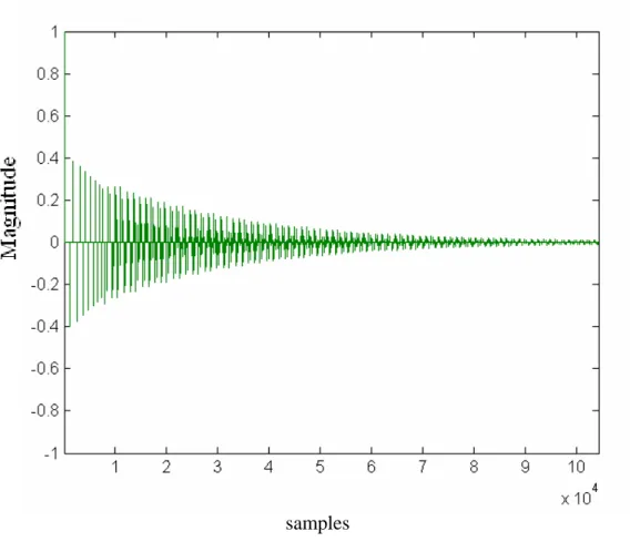
![Figure 10. The impulse response by using image-source method with n=30, room dimension = [10 8 3] and absorption coefficient is 0.8](https://thumb-ap.123doks.com/thumbv2/9libinfo/8462907.183251/60.892.139.755.256.707/figure-impulse-response-source-method-dimension-absorption-coefficient.webp)
