Abstract
Uni-axial compression test has been the general way to evaluate the strength of bulk materials, especially brittle materials, for decades. In the field of concrete or rock mechanics, compression strength is one of the most significant engineering characteristics. By observing the compression test of a cubic specimen, the most severe compression area in material (the inner central area), however, does not match the damage pattern (side wedge peeling). In the present study, the Discrete Element Method (so-called DEM or Particle Element Method) is employed to analyse a brittle block. One of the important advantages of this method is that material damage due to bonding and friction failure can be better described. In this paper, the results of elasticity, compression strength, and the crack profile of the bulk specimen are carried out using the two-dimensional discrete element method. Upon matching the numerical results to those of the lab test, one can determine the internal material parameters such as bonding strength, the frictional angle, and equivalent stiffness between particles in micro scale.
Keywords: uni-axial compression test, FEM, Mohr-Coulomb criterion, discrete element method.
1 Introduction
It is well known that Mohr’s Circle is an excellent tool to describe multi-axial stresses. Mohr-Coulomb’s failure criterion is one of the popular applications to rule the material failure mechanism under multi-axial stress condition. As stated in Mohr-Coulomb criterion, even if the specimen is subject to compression, or more specifically uni-axial compression, some portion of the specimen is failing by shear or tensile crack. For those specimens that particles are the main contents, are proven to be Mohr-Coulomb types of material. It is also appropriate for some brittle materials such as stone (especially sand stone).
Paper 131
The Failure Mechanism of a
Concrete Cube
C.C. Yu, S.H. Tung and M.C. Weng
Department of Civil and Environmental Engineering
National University of Kaohsiung, Taiwan ROC
©Civil-Comp Press, 2008
Proceedings of the Sixth International Conference on Engineering Computational Technology, M. Papadrakakis and B.H.V. Topping, (Editors), Civil-Comp Press, Stirlingshire, Scotland
Concrete is one kind of composites whose mechanical behaviour is quite complicated. Compressive strength and tensile strength are the major material failure parameters. In certain research cases like seismic analyses, shear strength may also be taken into account. These parameters are determined experimentally, compression strength by compression tests, tensile strength by tensile tests or three-point-bending tests, for examples. Since the tensile strength of concrete is much less than its compression strength, in general, concrete is assumed to have only the compression strength. Structures are often designed based on its compression strength only. Once the pressure in concrete reaches such compression limit, material is treated as fails.
By observing the compression test of a cubic specimen, the most severe compression area in material (the inner central area), however, does not match the damage pattern (side wedge peeling). Such a compression failure might just be a frictional slip in certain plane that the maximum friction resistance is controlled by Mohr-Coulomb criterion. The angle between the normal of such plane and the minimum principal stress axis is ±(π/4-φ/2). In order to see how it works for concrete, two numerical tools, traditional Finite Element Method (FEM) and Discrete Element Method (DEM), are employed to analyse a concrete cube subject to uni-axial compression. Two numerical results as well as the lab test result will be compared with each other in the present study.
2 Brief Review
2.1 Soil Failure and Mohr-Coulomb Criterion
By Mohr-Coulomb criterion, failure occurs if the shear stress in any direction is greater than a critical value related to its normal stress at the same location on the same plane. The critical value of the shear stress is plotted in Figure 1 as a straight line. To obtain such a critical line, soil specimens are tested until fail, at different pressure levels with different stress combinations, with or without circumferential stresses. Those ultimate stress states are expressed as Mohr’s Circles in stress space. The envelope to those Mohr’s Circles is approximately a straight line. A straight line is a nice approach and can be written as equation (1),
τ =c-σ tan φ (1) where c and φ are material constants representing cohesion (or pure shear strength)
and friction angle respectively.
Under the circumstance when tensile stress reaches the corresponding strength and dominates the failure, Rankine’s tensile failure criterion is to be utilized to better describe the realistic material behaviour. Mohr-Coulomb theorem combined with Rankine’s theorem therefore forms a complete failure criterion to regulate soil behaviours, including tensile (cracking) failure and compression (shearing slip)
failure. The crack surface in tensile failure is perpendicular to the maximum tensile stress. On the other hand, the slipping face in shear failure is not necessary the same face as the maximum shear stress occurs because not only shear stress but also compressive stress plays an important role [1-2].
2.2 Rock Strength and Failure
Similar situation mentioned above also applies to solid material, like rock or concrete. From engineering point of view, there are several definitions for material failure: certain stress component reaches its critical value (as stated in the previous section); certain strains reach their limits (2% yield limit for steel and 0.2% for concrete, for examples); the accumulated strain energy reaches it limit (J-Integral or Energy Release Rate G, for examples), etc. For solid material like rock or concrete, some popular failure criteria are Mohr criterion, Mohr-Coulomb criterion, Griffith theory, Hoek-Brown empirical failure criterion, and so on [3].
Most of the failure criteria used for solid material have an assumption that the specimen is homogeneous continuum with no defect (crack) in side. In fact, most of brittle materials are not flawless. Many researchers noticed [3] that based on the study of Griffith in 1921, micro cracks in brittle material may initiate and merge to form a fatal damage in particular failure environment.
Based on a large amount of experimental data from rock tests, Hoek and Brown [4] developed an empirical failure criterion, a parabolic failure envelope, to describe the failure behaviour of rocks. According to their study, the post failure stress-strain curve for brittle material is very complicated and it is hard to perfectly describe the behaviour using existing mechanics theorems.
The stress-strain relations for the uni-axial compression tests of a rock can be categorized into three groups (Figure 2): (1) perfectly plasticity, (2) elastic-brittle plasticity, and (3) elastic-softening plasticity. The main differences are that they have different post-failure stress-strain behaviours. Elastic-perfectly plasticity keeps the stress level after yielding point but stiffness vanishes. Both strength and stiffness of elastic-brittle plastic material drops down dramatically beyond ultimate
Figure 1. Mohr-Coulomb failure criterion for multi-axial stresses
σ τ
Failure Envelope Ultimate Mohr’s Circles
stress while elastic-softening plastic material decreases its strength and stiffness gradually after yield. Special caution must be taken carefully. The lab test control or numerical simulation for all three kinds of post-failure behaviors must be displacement-controlled. Rapid drop in strength and/or stiffness may cause system instability and incorrect data or data missing.
In the present analysis, a concrete cube will be treated in a similar manner as considered above since concrete cube is somewhat similar to a rock specimen.
3 Uni-Axial Compression Lab Tests
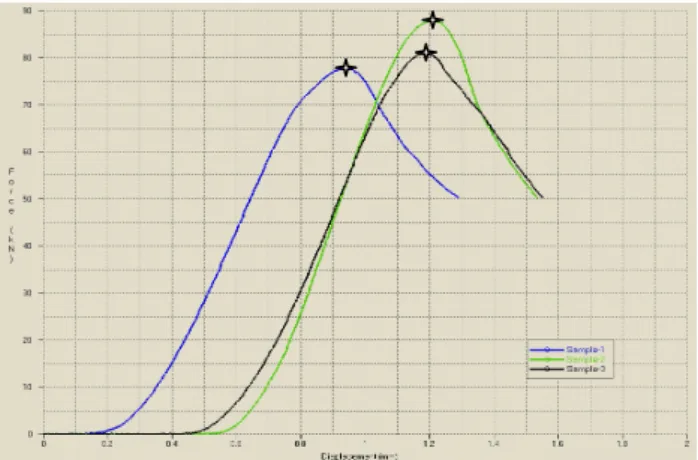
According to ISRM suggestion, the concrete cube specimen shall have the surface smoothness of less than 0.02mm. Fracture shall be achieved within 5-10 minutes. The dimension of a concrete cube specimen is 5cmx5cmx5cm. Specimens are made of cement, standard quartz sand, and water with the following weight ratios: ratio of sand to cement s/c=3 and ratio of water to cement w/c=0.6. The mortar is poured into and left in molds for three days, cured for two weeks after being removed from molds, and then left in room temperature to dry out for a few more days. They are tested for 21-day strength using a universal material testing system with a maximum capacity of 100 tons. The constant pressing rate is pre-set to 5x10⁻⁵ m/s. The force-displacement curves of the compression tests are shown in Figure 3. The peak value of each curve is taken as the strength of the corresponding specimen. The curve has a slow start because there is a small gap between specimen and compressing platen. Since no other extensometer (LVDT) or strain gauge is installed, the slope at the half strength of the stress-strain curve is taken as elastic (Young’s) modulus (Etan,50
of ISRM Code). During the test, data acquisition system automatically records loading force, displacement, stress, and strain histories. When entering yielding zone, the load-displacement curve becomes non-linear. In order to monitor the failure style, it is traced beyond failure and until the strain is at least 2% or more.
Lab test results show that the strain within elastic region is pretty small, which means the small deformation assumption in numerical analysis is reasonable. The average elastic modulus is E=3.269 GPa, mass density is ρ=3.5 g/cm3, average
ultimate loading force is Fu=82 kN. This comes up with an equivalent ultimate
stress of σu=33MPa. (1) (3) (2) ε σ
Figure 2. Three types of the stress-strain relations for the uni-axial compression tests: (1) elastic-perfectly plasticity, (2) elastic-brittle plasticity, and (3) elastic-softening plasticity.
Material post-failure behaviour for these specimens is between brittle-plasticity and softening-plasticity. By observing the shapes of the fracture surfaces (Figure 4a and 4b), one may find that the top and bottom faces of the specimens remain pretty much un-damaged. The central inner domain is still compact and the original shape is well kept. On four vertical faces of the specimens, material of wedge shape or shallow pyramid shape peels off and makes the rest of the specimens look like dumbbells.
This kind of wedge peeling off initiates from four corners of the contact faces, especially the upper contact face.
Figure 3. Force-displacement curves
Figure 4a. Fracture surfaces of a concrete cube
4 Numerical Approach
Two numerical methods are employed in the present analysis for comparison. One is continuum FEM (Ls-Dyna3D) using slow transient dynamic analysis to simulate semi-static loading condition. The other is DEM (PFC-2D) also using slow transient dynamic analysis. Note that the three-dimensional cube is simulated with solid elements in the former method while the two-dimensional square with cylindrical elements is considered in the latter method. The FEM result is just to demonstrate the stress distribution in a continuum cube before failure while the two-dimensional DEM model is to demonstrate the simplified fracture style after failure. The error coming from the dimension simplification in DEM case, therefore, shall be born in mind. Although the fracture mechanism is pretty complicated, by comparing the numerical results with lab test observation, one can qualitatively figure out the dominating factors in this case.
4.1 Finite Element Method and Results
The FEM approach is one of the most popular numerical methods accepted by researchers in many fields. The FEM model consists of 8000 eight-node constant stress solid elements. This deformable continuum is pressed down by a rigid platen from the top surface using displacement control with a constant pressing velocity as mentioned earlier. Through a semi-static procedure, the FEM output provides the distribution contours of various stress components. The major drawback for current FEM is that it is difficult to smoothly adjust the boundary condition to accommodate the new surface created by cracks. Users may need major modification in computer code in order to observe the crack propagation. The goal of the present study will be focused on the potential crack initiation location. For this particular job function, FEM with the assumption of continuous medium is still an excellent tool. Details will be further discussed later. The result is carried out first with linearly elastic material since its only purpose is to see the inner stress distribution before failure. Three types of boundary conditions are considered. One type of the boundary condition is that the nodes on the contact faces are fixed in two horizontal directions. Displacement is controlled in z- (vertical) direction. Another boundary condition is to assume that the upper contact face is frictionless. The other type of boundary condition assumes both contact faces frictionless. Young’s modulus, Poisson’s ratio, mass density, and displacement loading rate are the same as those for the lab test.
Three different kinds of boundary conditions lead to three totally different results. To show the contour in detail, the model is cut into several slices, from the outer face to the central inner layer. Fixed boundary results are illustrated in Figure 5 as vertical stress σzz contour in Figure 5a and von-Mises stress contour in Figure 5b.
Frictionless upper boundary results are shown in Figure 6 as vertical stress σzz
contour in Figure 6a and von-Mises stress contour in Figure 6b. With a frictionless upper contact face, the hot area moves upwards while most of the bottom surface is
still the cool area (or even cooler than in the fixed boundary case). If both contact surfaces are frictionless, the stress distribution is uniform. The variation in location is trivial in the third case and result is not presented in figure.
Other stress components are relatively small and are not shown in this paper. The stress levels are presented in contour figure with different colors from the highest to the lowest as red, pink, orange, yellow, green, blue, and black. Numbers are not shown because these figures are for qualitative discussion only. Frictionless contact face leads to a stress distribution that is not symmetrical with respect to the middle plane. It differs from the lab test observation. All of the damaged specimens after lab tests still have their near-perfect top and bottom contact face (Figure 4b). It means, the assumption that the contact is not frictionless is more reasonable. The discussion below will be focused on the fixed boundary case only.
Contour results show that the severely stressed areas are along the eight edges (especially at eight corner nodes) while the lowest stress occurs at the centers of the contact faces. This may explain why the fracture initiates at the corner nodes and along the edges but the contact faces remain un-damaged. Another severely stressed
Figure 5a. Contour of the normal stress σzz with fixed contact surface
Outer Slice Inner
Slice
Figure 6b. Contour of von-Mises stress with frictionless contact surface
Outer Slice Inner Slice Outer Slice Inner Slice
Figure 6a. Contour of the normal stress
zz
σ with frictionless contact surface
Figure 5b. Contour of von-Mises stress with fixed contact surface
Outer Slice Inner
region is at the central portion (the “heart”) of the cube. This does not fit in well with the lab test observation since most of the central regions of the specimens survive the tests. By re-doing the FEM analysis with another type of material: the Brittle-Damage Model, allowing a tensile limit of 12MPa, shear limit of 10.5MPa, fracture toughness of 8MPa, and shear retention of 4.5MPa, one can find that the stress distribution is not affected too much by the material changed before failure. Material failure starts from eight edges of the cube as expected. The most severe damage occurs at eight corner nodes. This phenomenon agrees with the previous linearly elastic FEM and lab test results. However, after fracture initiates, the layers near the contact faces are the consequent failure areas. The model is shortened not because of the damage in the heart area but because the first layers adjacent to the contact surfaces are flattened. Such post failure behaviour does not agree with the linear-elastic FEM result or the lab test observation and is not quite expected. That is, the explanation to the failure mechanism cannot be fully based on the stress distributions of either σzzor von Mises stress. There must be something else to be
taken into account.
4.2 Discrete Element Method and Results
To deal with the displacement field that involves discontinuity such as crack (either opening or slipping crack), the a useful tool is DEM. The original concept of DEM is raised by Cundall in 1971 [5] for solving discrete domain problem. One of his sample discrete element is the two-dimensional cylindrical element [6]. Large displacement, rotation, or even total separation is allowed between elements. According to material property and element geometry, there might be different kinds of external loads, including body force, contact force, bonding force, etc. All the loads acting at an element are calculated and added up to form the resultant force. Resultant force can be converted into acceleration using the second Newton’s law and therefore the velocity and displacement increments of that element can be determined by finite difference method. Because both FEM or DEM employed here uses explicit time domain integration, the stability and convergence of the numerical result sensitively depend on the size of the time step [7]. Fortunately, due to the excellent progress in both processing speed and memory space of the modern computer, this large amount of calculation becomes feasible.
If the forces between elements include gravity, normal contact forces, and friction forces only, DEM is a nice tool to analyze soil mechanics problem or particle flowproblem since in these problems, particles are allowed to transport separately. If in addition, the bonding force is also taken into account, particles may aggregate and move together like a one-piece body, yet it is still deformable. This method is pretty suitable to simulate the sliding of particles soaking in a continuous medium. It considers the possibilities for both shearing slip and tensile opening. Concrete with sand or stones, atoms in metal, and damaged rocks in clay soil all become appropriate objects for this method to simulate. The bonding strength is one of the key parameters of a successful simulation for the fracture problem of a continuum
[8]. It is good for such a problem particularly because of its capability to create new boundaries in any proper direction.
The contact between two discrete elements in current numerical analysis can be treated as two sets of equivalent spring and damper systems. One is normal to the contact surface and the other is in tangential direction (Figure 7). The out of plane tangential direction is not in the scope of this paper since this is a two-dimensional analysis.
People usually assume that the interaction between two similar bodies with smooth surface is Herzian contact. The magnitude of the Herzian contact force normally is a function of the contact area (or the relative approaching distance). The equivalent spring theoretically shall be a non-linear spring. However, the realistic situation is, the interaction force is not just caused by contact but also induced by pressing matrix material that the particles soaked in. In the present study, sands are the particle elements and cement-water compound is matrix material, i.e. major part of the spring. The interaction between particles is complicated. To simplify the problem and to save the computer resources, it would be reasonable to assume that the equivalent spring is linear.
In Figure 7, parameters kn and cn represent spring stiffness and damping
coefficient, respectively, in normal direction while ks and cs are spring stiffness and
damping coefficient in tangential direction. Elements connect with each other through those springs whose tensile strengths can be specified so that when the spring is subject to a tensile force higher than its strength, this spring is no longer functioning. One element may have as many springs as needed depending on how many other elements are in contact with this element. If all the springs of an element are broken, then the element can go free. The only interactions left between this element and other elements are the contact pressure and the friction force that comes with the normal pressure and complies with the Coulomb friction coefficient relation.
Since spring is employed to represent the interaction between elements, the overall behavior of bulk material, such as strength and Young’s modulus, can be tuned by adjusting the bonding strength of the spring and its stiffness. For example,
Figure 7. Equivalent Spring and Damper between elements
cs、ks
if both stiffness and bonding strength are set to fairly large numbers, bulk material behaves like a rigid body. If bonding strength is set to a very small number, the overall behavior will be more like sand. On the other hand, if strength is set to a large number but stiffness is set to a small number, the bulk body behaves like a soft sponge. These are some extreme cases. In general, these parameters shall be carefully tuned between extreme cases so that bulk material can have reasonable realistic behavior.
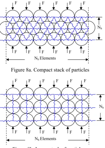
In numerical analysis, stiffness of the internal equivalent spring is one of the input data but in lab test, one can only obtain Young’s modulus and ultimate strength of the bulk cube. In the present two-dimensional case, in order to estimate theoretical Young’s modulus for bulk material, a net made of springs connecting all the centers of elements is shown in Figure 8. Figure 8a illustrates the most condensed stack of elements. Figure 8b shows another loose stack. Overall Young’s modulus can be obtained by calculating the total external force and the global displacement. Young’s modulus obtained in this way is just approximate. The actual element arrangement in later numerical analysis is randomized and there could be cavities inside the bulk. Yet, Young’s moduli obtained from these two stacks are still good references for later analysis. They will also be the initial guess for the later detailed parametric study.
Figure 8a. Compact stack of particles
Nb Elements F F F F F F F F F F F F Nh F F F F F F F F F F F F
Figure 8b. Loose stack of particles
Nh
In compact stack in Figure 8a, the system can be treated as a truss structure with each spring as a truss member. Due to the symmetry, this structure can also be disassembled into several identical units, each of which is a triangular simple truss as shown in Figure 9. The member forces of three springs in each unit can be determined by applying symmetry and equilibrium conditions. Result is also shown in Figure 9. The positive sign means tension and the negative sign means compression. By any structural analysis method (unit load method, for example), the vertical displacement can be calculated as
n k F 4 3 =
Δ . For the entire bulk, the total vertical displacement is h n N k F 4 3 =
Δ . Also for the entire bulk, the total external load is P=NbF, total height is L= 3RNh , and, with unit thickness in the direction
perpendicular to the paper, the total cross section area is A=2RNb. Thus, the
equivalent overall Young’s Modulus is kn
3 2 A PL E = Δ = .
Similarly, in loose stack in Figure 8b, the structure is actually a parallel-serial multi-spring system. The member internal force is f=F, total vertical displacement is
h n N k F =
Δ , total external load is P=NbF, total height L=2RNh, total cross section area
A=2RNb, and thus Young’s modulus is equivalent to E= ΔPLA =kn.
Young’s modulus is linearly related to kn in this case. In general, Young’s
modulus may range between these two theoretical values, i.e. n kn
3 2 E
k ≤ ≤ . Note that, here, material is assumed to be homogeneous. The variety of the size of particles and the large cavity formed by a loop of particles is not taken into account. Therefore, the theoretical values of Young’s modulus are just for approximate reference. In the later analysis, the process is actually reversed. First, a realistic value of Young’s modulus is determined in lab test. Using the relation between Young’s modulus and kn to estimate the internal parameter kn. Put this kn into
F F/2 F/2 3 F f = − 3 2 F f = 3 F f = −
Figure 9. Triangular simple truss and the corresponding member forces
numerical model and obtain global Young’s modulus. Adjust kn by comparing
numerical result to the lab test result. The relation between global ultimate load and internal bonding strength is more complicated because the former is influenced sensitively by local stress concentration and local damage. It is not simply the summation of the contribution from all springs. It will be a trial-and-error process to determine the internal bonding strength.
The commercial computer code PFC2D (Particle Flow Code in 2 Dimensions) was developed by Itasca Inc. based on the DEM theory. The base units, circular elements, are stacked to form any particular bulk shape. Here, element is the so-called “particle” represented by its center with a radius value indicating its size. When particles collide into one another, the contact is treated as inelastic because of the existence of friction and damping. The contact behaviour is ruled mainly by two springs, one in normal direction and the other in tangential direction. Friction force Fs exists and bounded by friction coefficient μ as Fs≦μFn where Fn is the normal
contact force.
The geometry of the particles offers quite a bit of influence to the contact behaviour. Many researchers try elliptic particles [9-12] and arbitrary polygons [13] to figure out how the shape of the particles affects the numerical result. The major difficulty for the non-circular particle analysis is the complexity in contact interface scheme. For simplification purpose, the two-dimensional cylinders are used in the present analysis. PFC also provides two types of bonding models: the contact-bond model and the parallel-bond model. The former offers the initial bonding strength in both normal and tangential directions. The latter provides a beam between two particles. Such a beam takes not only normal and tangential forces but also the bending and torsion into account.
Unless specified otherwise, some parameters used in the DEM analysis in this paper are: kn=1x10⁶ kN/m, ks=2.083x10⁵ kN/m, Bonding strength σb=32 kPa/m,
cavity ratio 0.15, and contact friction angle 20°. The model is a two-dimensional bulk with the dimensions of 0.05m*0.05m*1m. Time step is set to Δt=1x10⁻⁵
second. The numerical procedure is as follows.
(1). Fill the container whose dimensions are specified in previous paragraph with elements (cylinders in this study).
(2). Adjust the radius of elements so that the specified cavity ratio can be met. (3). Check unbalanced elements and give a period of time for natural relaxation and
condensation.
(4). Initialize bonding strength.
(5). Remove sidewalls of the container so that four vertical faces of the specimen become traction free.
(6). Give another period of time for natural relaxation.
(7). The top and bottom walls of the container move slowly toward each other at a constant speed until the specimen fails.
5 Discussions
Based on the FEM result, high compressive vertical stress occurs along eight edges and at the center of the model. Lab test shows that crack initiates from the edges, propagates into specimen, and causes surface chips to peel off. The vertical stress distribution does not match with the observation of the lab test. The statement: “Concrete fails if material reaches its compressive strength.” may not be fully appropriate. Similar situation also applies to the distribution of von-Mises stress as well. High von-Mises stress occurs along eight edges and at the center of the model. The failure mechanism cannot be explained solely by compressive stress σzz or
von-Mises stress. The Mohr-Coulomb failure criterion, therefore, becomes a candidate for reasoning such failure phenomenon.
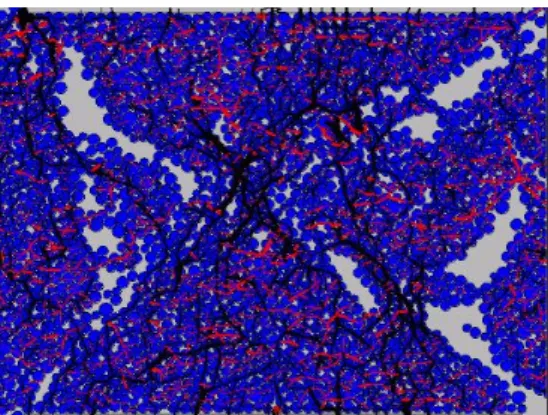
Figure 10a shows the model before failure. Figure 10b shows the specimen after failure. Because the top and bottom surface are constrained in two horizontal directions, there are two triangular regions adjacent to these two contact surfaces remain pretty much un-damaged. Vertical surfaces peel off in wedges just like what is observed in lab test. The central area still carries most of the vertical pressure after failure.
Figure 11 is captured and magnified from local area (as marked by a dotted line) in Figure 10a. The black lines in this figure represent the compressive forces between elements due to contact pressure. Red lines are tensile forces before de-bonding. The bolder the line is, the higher the force is. One can see that the black lines spread all over the entire domain in this figure and they join into one another forming a continuous net. This means, compression is the dominant force. Some black lines form a grid shape of diamonds. It implies that the elements are in compact stack as in Figure 8a. Some black lines are vertical and parallel to each other. It means the elements are in loose stack as in Figure 8b. The interesting thing is, even in such a compression situation, there are still many red segments.
Figure 10b. Compressed model after failure
Basically most of the red segments are horizontal and remain short and independent and do not merge into lines.
Young’s modulus E for bulk material is plotted in Figure 12 as a function of internal spring stiffness kn. In this parametric study, tangential stiffness ks is
proportionally adjusted, i.e. Δks/ks=Δkn/kn. Result shows that E and kn are linearly
related to each other. The correlation factor is R2=0.9969. The slope of the E-kn
curve is dE/dkn=2.123. This value is not equal to that in the previous estimation
using simple truss model shown in Figure 8 (dE/dkn=1.16). Possible reason is that
ks and friction are not considered in truss model.
Other important parameters that affect the overall ultimate strength are internal friction angle ψ and internal bonding strength. Results are illustrated in Figure 13 and 14 respectively. Both parameters are linearly related to P as well. For the concrete cube used in lab test, ultimate stress is σu=33MPa and Young’s modulus is
E=3.269 GPa. If the internal friction angle is assumed to be ψ=20°, the equivalent values for kn and σb are kn=9x10⁵ kN/m andσb =22 kPa/m.
Figure 11. Local area captured from Figure 10a
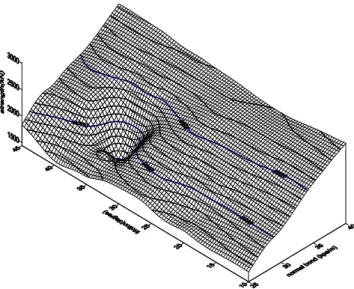
Let P be a function of ψ and σb. Figure 15 shows the relation among these three
variables. For most of the values of ψ and σb, P is linearly proportional to these two
parameters (i.e. a plane surface), the ultimate strength P is particularly low when ψ ranges from 35° to 40° and the bonding stressσb is at around 30kPa/m. Further
study is required to figure out why.
6 Conclusions
The term “Compression strength” does not correctly describe property of concrete. In fact, the failure mechanism cannot be explained solely by compressive stress σzz
or von-Mises stress. Several material parameters may affect the ultimate strength. Figure 14. Ultimate load P for bulk material
as a function of internal bonding stress σb
ψ (Degree)
Figure 13. Ultimate load P for bulk material as a function of internal friction angle ψ
Mohr-Coulomb criterion offers a better explanation for the failure mechanism of concrete.
By DEM, a concrete cube, in the present analysis, consists of a lot of two-dimensional particles. The contacts between particles are handled by using the equivalent springs. By carefully choosing the appropriate values of parameters kn,
ks, σb, and ψ, the simulated fracture profile is in fair agreement with the lab test
result. On the other hand, the internal parameters kn, ks, σb, and ψcan be determined
by comparing Young’s modulus, overall compressive strength, and the fracture profile of the the numerical model to those of the lab test specimen. A set of the parameters are found to be able to describe the cube specimen behavior fairly well. They are internal friction angle ψ=20°, equivalent spring stiffness kn=9x10⁵ kN/m
and normal bonding strength σb =22 kPa/m. Of course, there are many parameters
that may affect the result and there could be some other set of the parameters that can fit the behaviour better.
As some of the interesting future research, it would be worth the efforts to correlate the overall compressive strength with volume change, critical strain, the pattern of the particle stack, mixed sizes of particles, etc. Another interesting future topic is to re-solve the question why there is a dent on the surface of ultimate load P as a function of ψ and σb when ψ ranges from 35° to 40° and the bonding stressσb is
at around 30kPa/m (Figure 15).
References
[1] C.-L. Huang, Concrete Property and Behavior, in Chinese, Chan’s Arch Books Co., LTD., Taipei, Taiwan, 1997.
[2] C.-C. Lin, Analysis on Cement Mortar Strength Parameters c and φ , in Chinese, master thesis, Graduate Institute of Civil and Disaster Prevention Engineering, National Taipei University of Technology, Taipei, Taiwan, 2003. [3] K.-C. Shih, Rock Mechanics, in Chinese, WenSheng Book Store, Taipei,
Taiwan, 1999.
[4] E. Hoek and E. T. Brown, ”Undergrown excavations in rock,” Institute of Mining and Metallurgy, Lodon, 1980.
[5] P. A. Cundall, “A computer model for simulating progressive, large scale movement in blocky rock systems,” Proc.,Symp. Int. Soc. Rock Mech., Inst. Civ. Engrg., Nancy, France, 2(8), 129-136, 1971.
[6] P. A. Cundall and O. D. L. Strack, “A discrete numerical model for granular assemblies,” Geotechnique, London, England, 29(1), 47-65, 1979.
[7] B. M. Das, Principles of Foundation Engineering, PWS-KENT, Boston, USA, 221-285, 1993.
[8] M. Hakuno and K. Meguro, “Simulation of the Collapse of Concrete Frames and Volcanic Eruption,” Advances in Micromechanics of Granular Materials, Elsevier Science Publishers B. V., 321-330, 1992.
[9] C.-Y. Wang and V.-C. Liang, “A Packing Generation Scheme for the Granular Assemblies With Planar Elliptical Particles,” International Journal for Numerical and Analytical Methods in Geomechanics, 21, 347-358, 1997.
[10] T.-L. Lee, Numerical Simulation of the Motions of the Elliptic Particles, in Chinese, Master Thesis, Graduate Institute of Applied Geology, National Central University, Chungli, Taiwan, 1997.
[11] L. Rothenburg and R. J. Bathurst, “Analytical study of induced anisotropy an idealized granular material, “ Geotechnique, 39(4), 601-614, 1989.
[12] L. Rothenburg and R. J. Bathurst, “Numerical Simulation of Idealized Granular Assemblies With Plane Elliptical Particles,”Computers and Geotechnics, 11, 315-329, 1991.
[13] T. X. Tran and R. B. Nelson, “Analysis of Disjoint Two-Dimensional Particle Assemblies,” J. of Engineering Mechanics, ASCE, 122(12), 1139-1148, 1996.