慢性B型肝炎病毒感染之年齡相關模型及存活機率分析 - 政大學術集成

全文

(1)國立政治大學應用數學系碩士學位論文 . . sit. io. n. al. er. Nat. 及存活機率分析. y. ‧. ‧ 國. 學. 治 with Survival An Age-Dependent 政 Model 大 Analysis on立Chronic Hepatitis B Virus Infection 慢性 B 型肝炎病毒感染之年齡相關模型. Ch. e n g c h i. i n U. v. 碩士班學生：陳炘毓撰 . 指導教授：陸行博士中華民國九十九年九月 .

(2) Contents 謝辭................................................................................................................................. i Abstract .......................................................................................................................... ii 中文摘要....................................................................................................................... iii List of Figures ............................................................................................................... iv List of Tables ................................................................................................................. vi 1 . Introduction ............................................................................................................ 1 . 2. A Life Table and Semi-Markov Chains .................................................................. 4. 政治大 2.2 Markov Chain .................................................................................................. 7 立. 2.1 A Quick Review of A HBV Progression Model............................................... 4. ‧ 國. 學. 2.3 Chapman-Kolmogorov Equations ................................................................. 10 2.4 The Life Table ................................................................................................ 12. ‧. 2.5 Markov Renewal Chains and Semi-Markov Chains ...................................... 15 Model Structure ................................................................................................... 20. sit. y. Nat. 3 . n. al. er. io. 3.1 The Revised Life Table .................................................................................. 20. i n U. v. 3.2 The Construction of The Proposed Model ..................................................... 26. Ch. engchi. 3.3 Computation Methods .................................................................................... 31 4 . Numerical Experiments and Analysis .................................................................. 34. 5 . Conclusion ........................................................................................................... 69 Appendix .............................................................................................................. 70 References ............................................................................................................ 74 . 2 .

(3) . 謝辭這篇論文經過了接近一年半的努力終於完成，首先要感謝的我的指導教授陸行老師。老師在作研究方面的熱誠、成就以及知名度並不是三言兩語可以形容的，在加入陸行老師的研究團隊之前，我從來沒有想過自己可以涉及到醫學方面的研究，確確實實的是在應用數學。感謝老師在此篇論文上的寫作指導，經過了十多次的修正、修改、及潤飾文章，最終是完成了這篇論文。也感謝陳政輝老師不遺餘力的教導，幾乎可以算是我另外一位指導教授。這個作業研究團隊不像其他研. 政治大. 究團隊般的嚴肅，每一次討論皆是在輕鬆的氣氛下度過。也感謝長庚醫院以及簡. 立. 榮南醫師的配合、指導、以及合力研究，讓我們更是直接的面對到我們的研究目. ‧ 國. 學. 標。. 感謝所有在求學過程中陪伴我的同學，感謝黃國倫、林政憲、王伊君從大學. ‧. 到研究所的陪伴，我會永遠記得大家一起念書一起出去玩的日子。感謝曾琬甯、. y. Nat. n. al. er. io. 這些日子的。. sit. 李宣緯在寫論文時的共患難。也感謝常一起出遊的研究所同學們，我也不會忘記. i n U. v. 特別感謝林政憲、曾琬甯協助我統計方面的知識讓這篇論文更加完整。也感. Ch. engchi. 謝行政院國家科學委員會補助，計畫編號 NSC 98-2221-E-004-001-MY2。最後感謝我的家人，讓我可以心無旁騖的在政大渡過求學的這六年，完成我的大學以及研究所學業，謝謝！. 陳炘毓. 謹誌. 國立政治大學應用數學所中華民國九十九年十月 i .

(4) . Abstract In this thesis, we propose a new mathematical model extending the natural history of hepatitis B virus (HBV) prognosis progression on chronic HBV infection. Since the actual transition probabilities between symptoms are dependent of ages, it has been proposed that the life table should be accommodated to the HBV prognosis progression model so that it can more properly explain the disease progression of the HBV patients. But in the literature, no further disease analysis and applications of it. 政治大 progression is described by立 a Markov model, and propose a new method to combine. with the life table are discussed. In this thesis, we assume that the original disease. ‧ 國. 學. the HBV progression with the life table so that the proposed model integrates data from the life table and allows the accommodation of age-dependent properties of the. ‧. target disease. With clinical data based on annual incidence rates, the entire model is. sit. y. Nat. Semi-Markov based in nature. Computation methods similar to the celebrated. n. al. er. io. Chapman-Kolmogorov equation can be applied to study the associated probability of. i n U. v. each likely trajectory with desired initial ages and health states under the scenarios of. Ch. engchi. natural history and various treatment policies. This method provides a more accurate way to analyze the transitions between symptoms, such as the mean life expectancy or the survival probabilities at different ages. We will give examples to demonstrate the proposed method in this thesis. Numerical results show the proposed model not only provides a more accurate method to analyze the mean life expectancy, the survival probabilities at different ages, and the transition probabilities from symptoms to death but also helps us to understand the transitions between symptoms.. ii .

(5) . 中文摘要在此篇論文中，我們提出一個慢性Ｂ型肝炎病毒感染病程之數學模型。因為在病症間的轉移機率(Transition probability)是隨著患者的年齡變動，所以在過去的文獻中，已經有學者提出，在疾病轉移機率模型中，應加入國民生命表(Life table)，藉此讓機率模型更符合Ｂ型肝炎病患的生命歷程。但是過去的文獻中，學者並沒有利用加入國民生命表之後疾病模型做進一步的病程分析。在這篇論文當中，我們假設原始的疾病轉移模型是符合馬可夫鏈的性質，並且提出一種加入國民生命. 政治大我們使用著名的Chapman-Kolmogorov公式計算Ｂ型肝炎的自然病程機率，並畫立. 表的方法，賦予疾病有年齡相關特性之模型。根據文獻數據和類馬可夫機率性質，. ‧ 國. 學. 出病人的生存機率曲線(Survival curve)。文章最後將會藉由兩個例子來介紹此篇論文提出的模型。實驗數據結果證實，此模型不僅提供了一個更精確的方法去分. ‧. 析在病症與死亡間的轉移機率、平均餘命(Life expectancy)、以及在不同年齡的存. y. sit. n. al. er. io. 移狀況。. Nat. 活機率(Survival probability)，並且可以更進一步的分析且瞭解病情狀態之間的轉. Ch. engchi. iii . i n U. v.

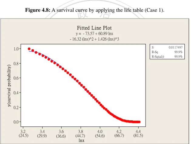
(6) . List of Figures Chapter 2 2.1. Figure 2.1 A model on HBV infection from Liaw and Chu [19]………………5. Chapter 3 2.1. The revised mortality from the original life table [30]…………………………24. 2.2. The survival function …….……………………………………………………25. 2.3. An illustrated example of the proposed model……………….…………….….27. 立. ‧ 國. 學. Chapter 4. 政治大. The new transition diagram.…………………..…………………………….35. 4.2. The mortality of a person who had the HBV infection (Case 1)…….………...38. 4.3. The mortality of a person who had the HBV infection (Case 2)…….………...39. 4.4. The survival probability of a person who had the HBV infection at age. ‧. 4.1. n. er. io. sit. y. Nat. al. i n U. v. 25 (Case 1)...……………………….…………….……………………...……..40 4.5. Ch. engchi. The survival probability of a person who had the HBV infection at age 25 (Case 2)…………………...……...……………………………………...….41. 4.6. The survival probability of different ages starting at age 25 by applying the life table (Case 1)………………..………..……………………..…..……..44. 4.7. The survival probability of different ages starting at age 25 by applying the life table (Case 2)….…………..…………………...………………………45. 4.8. A survival curve by applying the life table (Case 1)……………...……………47. 4.9. A survival curve by applying the life table (Case 2).…………..………………48. 4.10 An alternative interpretation for the transition diagram of Figure 4.1….....51 iv .

(7) . 4.11 The original transition diagram………………...……………………...……..53 4.12 The transition diagram after separation…………...………………………….53 4.13 The mortality of a person who had the HBV infection at age 25 (Case 3)…….54 4.14 The mortality of a person who had the HBV infection at age 25 (Case 4)…….55 4.15 The survival probability of a person who had the HBV infection at age 25 (Case 3)………………...…………………………………………………...56 4.16 The survival probability of a person who had the HBV infection at age 25 (Case 4)…...………………………...……………………....................……57. 政治大 the life table (Case 3)..………………………..……………………………......58 立. 4.17 The survival probability of different ages starting at age 25 by applying. 4.18 The survival probability of different ages starting at age 25 by applying. ‧ 國. 學. the life table (Case 4)..…………………..…………………………………..…59. ‧. 4.19 A survival curve by applying the life Table (Case 3)…………...……...………60. sit er. al. v i n Ch A simple model of HBV infection………………...……………………………69 engchi U n. 1. io. Appendix. y. Nat. 4.20 A survival curve by applying the life Table (Case 4)……...………...…………61. v .

(8) . List of Tables Chapter 2 2.1 The symbols of states………………………………………………………..…..6 2.2 The life table (excerpted from the original life table [30])...……………..…….14. Chapter 3 3.1 Illustration of the revised life table………………………...……………..…..22. 立. Chapter 4. 政治大. ‧ 國. 學. 4.1 Summarized results of Case 1 and Case 2 without the life table………..…..…41 4.2 Summarized results of Case 1 and Case 2 with the life table………..…….…..46. ‧. 4.3 The 95% confidence interval for life expectancy in Case 1 and Case 2…….....46. sit. y. Nat. 4.4 The ANOVA table for Case 1……..…………………………………..……….49. n. al. er. io. 4.5 The sequential analysis of variance for Case 1. ……………….………………49. i n U. v. 4.6 The ANOVA table for Case 2. …………………………………………...……50. Ch. engchi. 4.7 The sequential analysis of variance for Case 2..…………………...………..…50 4.8 The symbols of states for Case 3 and 4………………………………...……....52 4.9 Summarized results of Case 3 and Case 4 without the life table………………57 4.10 Summarized results of Case 3 and Case 4 with the life table……………….…59 4.11 The 95% confidence interval for life expectancy in Case 3 and Case 4…….....60 4.12 The ANOVA table for Case 3. ………………………………………………...62 4.13 The sequential analysis of variance for Case 3. ……………………………….62 4.14 The ANOVA table for Case 4..………………………………………………...63 4.15 The sequential analysis of variance for Case 4..……………………………….63 vi .

(9) . 4.16 The regression models for transition between some symptoms.........................65 4.17 The demonstration of the application (1)…………...………………………….65 4.18 The demonstration of the application (2)…………...………………………….66 4.19 The demonstration of the application (3)………………………………………68. 立. 政治大. ‧. ‧ 國. 學. n. er. io. sit. y. Nat. al. Ch. engchi. vii . i n U. v.

(10) . Chapter 1. Introduction Beck and Pauker [4] have proposed a model applying a life table to the original disease progression model according to exponential distribution property, indicating the population mortality does play an important role in survival analysis. Among the. 政治大 infection prognosis progression model is described in Liaw and Chu [19]. Though this 立. literature regarding hepatitis B virus infection (HBV), one of the most popular HBV. model provides a very important guideline to the progression of chronic HBV. ‧ 國. 學. infection, it is not easy to derive for applications such as patients’ survival analysis. ‧. and cost-effectiveness analysis on different therapies. In this thesis, we propose a. sit. y. Nat. more general model extended from this original model. In the proposed model, data. io. er. from the life table is included. It naturally embeds the non-uniform age-specific mortality into the model. When age-dependent disease related properties are. n. al. Ch. concerned, the model can be easily adjusted. engchi. v i n and U provides. a more accurate. approximation to the realistic situations.. Recent works in disease progression analysis have focused on cost effectiveness [14,18,23], medical treatment decision making [13], or the natural histories of diseases [9,11]. Many mathematical methods are applied to help analyzing the relative medical problem and the natural histories of the diseases. Pwu and Chan [23] have used the decision tree and the Markov model to analyze to cost effectiveness for the treatments of chronic HBV. Markov cohort method is used to construct transition 1 .

(11) . probabilities from well to ill statuses or death [27]. The exponential distribution property plays an important role in combining the life table with the disease progression [4,18].. The two major different kinds of Markov processes are time-independent Markov chains and time-dependent Markov processes. We assume the disease progression belongs to one kind of Markov processes. According to the follow-up clinical anamneses, the epidemiologists conclude the annual transition rate between. 政治大 chains are always constant is not realistic in real disease progression models. It is easy 立 all enumerations of symptoms. However, assuming the transition rates of the Markov. to see that the mean life expectancy of an individual is dependent on age and. ‧ 國. 學. disease-adjusted mortality. Hence, the time-dependent Markov processes are. ‧. important in construction of a HBV model. Our proposed model not only adjusts the. sit. y. Nat. transition probabilities between clinical symptoms but also adjusts all the transition. io. al. n. Taiwan life table [30].. er. probabilities from well and ill states to death and reflects mortality with the light of. Ch. engchi. i n U. v. Since Liaw and Chu [19] gives a purely medicine-oriented article, its major focus is to summarize the long-term clinic observations and provide a guideline to the disease progression. Though many medical findings such that genotypes may affect the annual incidence rates are mentioned in the original article, their corresponding mathematical meanings and details are not well discussed, implying that none is developed from mathematical viewpoints. Our model is Semi-Markov based in nature. We will discuss the properties and applications of Semi-Markov process with HBV infection prognosis. When drug interventions or other contributing factors, which may 2 .

(12) . affect the transitional behavior, are taken into account, the proposed model can be easily tailored to reflect these alterations. In addition, the presented follow-up computation methods are applicable to these desirable variants.. In this thesis, first we construct the annual disease transition matrix according to Liaw and Chu [19]. Then we derive the revised transition probabilities by our proposed model, and compute the probability of the first hitting a specific health state with the life table. The survival curve with the life table follows afterwards. Finally,. 政治大. we present regression models of the survival curves.. 立. The remaining parts of this thesis are organized as follows. In Chapter 2, the. ‧ 國. 學. definition of the life table [30] will be stated and we make some important. ‧. assumptions by using the model of chronic HBV infection proposed in Liaw [19].. sit. y. Nat. Some properties and theorems of semi-Markov chain of the proposed model and the. io. er. computation method are also included in Chapter 2. In Chapter 3, first we revise the life table and explain the construction of the proposed model step by step. Then we. al. n. v i n Ccomputation. demonstrate how we conduct the give an illustration of examples of h e n g c We hi U this proposed model and analyze the results in Chapter 4. It summarizes our work and. draws some conclusion in Chapter 5. The introduction for chronic hepatitis B virus infection and its natural history are given in Appendix.. 3 .

(13) . Chapter 2. A Life Table and Semi-Markov Chains 2.1 A Quick Review of A HBV Progression Model. Understanding the mechanism of the progression of chronic HBV infection plays a. 政治大 effective therapies. It is summarized in Appendix. The progression of chronic HBV 立 very important role in its prevention. It also serves as a basis for the development of. infection can be represented graphically by Figure 2.1 proposed in Liaw [19]. We. ‧ 國. 學. suppose that the proposed model in Liaw [19] follows a Markov assumption. In this. ‧. model, the variations of some important clinic markers and histological outcomes are. sit. y. Nat. used to identify significant disease progression. Each state within this model. io. er. corresponds to one possible healthy status that patients may experience. The likely transitions between different states are specified by arrows as well as their associated. n. al. annual incidence rates (i.e.. i n C h transition rates.) annual A engchi U. v. trajectory consisting of. successive states represents the history of healthy statuses that a patient may experience chronically.. Though this model provides a very important guideline to the progression of chronic HBV infection, the stated model is oversimplified from mathematical and engineering viewpoints. For instance, in the same article, it mentioned that the transition rate from the state “HBeAg seroconversion” to the state “HBeAg(+) hepatitis HBV-DNA > 2 106 7 IU/mL” (called HBeAg reversion) is age-related. 4 .

(14) . However, even for healthy people, their morality rates are non-uniform over various ages. The infection of HBV complicates the situation. With the age-related morality and transitions involved, the non-uniform pattern is not accurately reflected in the original model since the mean life expectancy of an arbitrary initial state is difficult to be analyzed. In addition, for factors that could affect the transition rates, their corresponding mathematical details are not discussed in the original article. Due to such insufficiency, we propose a general framework, which integrates data from the life table, to more accurately approximate the non-uniform morality under HBV. 政治大 follow-up analysis methods such that these factors may be included in our framework. 立. infection. Furthermore, we present how this model can be adjusted as well as the. ‧ 國. 學. Figure 2.1: A model on HBV infection from Liaw and Chu [19].. ‧. n. er. io. sit. y. Nat. al. Ch. engchi. 5 . i n U. v.

(15) . In brief, we consider Figure 2.1 and classify it into 12 states. They are summarized in Table 2.1 below.. Table 2.1: The symbols of states. Symptoms. State symbol. HBeAg(+) hepatitis HBD-DNA> 2*10^6~7 IU/mL. s1. HBeAg(+) hepatitis HBD-DNA> 2*10^4~5 IU/mL. s2. HBeAg seroconversion. s3. 政治大立Remission. s4. HBeAg(-) hepatitis HBD-DNA> 2*10^3~4 IU/mL. ‧ 國. Decompensation. y. sit. HCC. io. n. Curative therapy. engchi U. Death/transplantation. 6 . er. Nat. Inactive carrier. Ch. s7. ‧. HBsAg loss. al. s6. 學. Liver cirrhosis. s5. v ni. s8 s9. s10 s11 s12.

(16) . 2.2 Markov Chain. Suppose that the proposed model in Liaw and Chu [19] is a Markov model and consider a stochastic process {Yn , n  1, 2,3,...} that takes on a finite or countable number of possible values. Specifically, this set of possible values of the process will be denoted by the set of a finite space E  {s1 , s2 , s3 ,..., s12 } . If Yn  i and i  E , then the process is said to be in state i at time n . Note that the 12th state represents death, or the end of HBV infection. Hence, in convenience, we denote E *  E  {s12 } . In the. 政治大. following sections, we denote  as the set of all positive integer for convenience.. 立. ‧ 國. 學. Theorem 2.1 Assume that whenever the process is in state i , there is a fixed probability Pi , j that it will next be in state j . That is, we suppose that. ‧. Pr{Yn 1  j | Yn  i, Yn 1  in 1 ,..., Y1  i1 , Y0  i0 }  Pi , j ,. (2.2.1). al. er. io. sit. y. Nat. for all states i0 , i1 ,…, i , j  E . Such a stochastic process is known as a Markov chain.. v. n. We summarize all the transition probabilities Pi , j as a transition probability matrix. P,. Ch. engchi. i n U. which is an m  m matrix. Equation (2.2.1) also tells us that the probability. from Yn to Yn 1 is only relative to Yn and is independent of the past states Y0 , Y1 ,… , Yn 1. , which is famous as a Markov property. The value Pi , j represents the probability. that the process will, when in state i , next make a transition into state j . Since probabilities are nonnegative and the process must make a transition into some state, we have that Pi , j  0, and. P jE. i, j.  1,  i  E * .. 7 . (2.2.2).

(17) . Definition 2.2 If i  E , the probability from state i to state i in one transition is 1, then we call state i is an absorbing state. That is, Pii  1 .. Therorem 2.3 Consider a Markov chain {Yn , n  1, 2,3,..., N } with finite state E and transition probability matrix P . Without loss of generality, we rearrange the elements of E and divide it into two sets A and B . Let A  {s1 ,..., sm } be the set of transient states and B  {sm 1 ,..., sN } be the set of absorbing states. Then the transition matrix can be expressed as p1,2 . p1, m 1.  . 立. p1, N    pm , N   Q R  , 0  0 I      0  1 . 治    政   大 p p . pm ,2 . ‧ 國. p1, m. m, m. m , m 1. 0. 1. 0 . . . 0.  .  .  0.  0.    0. 學.  p1,1     pm,1  P 0       0 . ‧. where Q  M mm , R  M m( N  m ) but 0  M ( N  m )m is a zero matrix, and I  M ( N  m )( N  m ) is. er. io. sit. y. Nat. the identity matrix.. Note that the elements of R are the one-step transition probabilities from. al. n. v i n states, C and the elements of Q are the hengchi U. transient to absorbing. one-step transition. probabilities among the transient states. Let U  [ukj ] , where ukj  lim Pr{Yn  j , j  B | Y0  k , k  A}. n . (2.2.3). It is seen that U is an m  ( N  m) matrix and its elements are the absorption probabilities for the various absorbing states from different transient states. Then it can be shown that U  ( I  Q ) 1 R  R.. (2.2.4). The matrix   ( I  Q) 1 is known as the fundamental matrix of the Markov chain. Let Dk denote the total time steps to absorption from transient state k . Let 8 .

(18) m. E ( Dk )    ki ,. k  1,..., m,. (2.2.5). i 1. where  ki is the element of  on the k th row and the i th column.. 立. 政治大. ‧. ‧ 國. 學. n. er. io. sit. y. Nat. al. Ch. engchi. 9 . i n U. v.

(19) . 2.3 Chapman-Kolmogorov Equations. The one-step transition probabilities Pi , j have already been defined. Now we define the n-step transition probabilities Pi ,( nj ) to be the probability that a process in state i will be in state j after n additional transitions. That is, Pi ,( nj )  Pr{Yn  k  j | Yk  i},. n  0, i, j  E.. (2.3.1). Clearly, Pi ,(1)j  Pi , j . The Champman-Kolmogorov (CK) equations provide a method for computing these n-step transition probabilities. These equations are . n, m  0, i, j  E. 政 治大. Pi ,( nj  m )   Pi ,(kn ) Pk(,mj ) , k 0. 立. (2.3.2). Equation (2.3.2) is most easily understood by noting that Pi ,(kn) Pk(,mj ) represents the. ‧ 國. 學. probability that starting in i the process will go to state j in n  m transitions through a path which takes it into state k at the nth transition. Hence, summing over. ‧. all intermediate states k yields the probability that the process will be in state j after. y. Nat. al . n. =  Pr{Yn  m  j , Yn  k | Y0  i} k 0 . Ch. engchi. er. io. Pi ,( nj  m )  Pr{Yn  m  j | Y0  i}. sit. n  m transitions. Formally, we have. i n U. v. =  Pr{Yn  m  j|Yn  k , Y0  i}Pr{Yn  k | Y0  i} k 0 . =  Pk(,mj ) Pi ,(kn ) . k 0. If we let P ( n ) denote the matrix of n-step transition probabilities Pi ,( nj ) , then the equation above asserts that P (n m)  P (n)  P (m) ,. (2.3.3). where the dot represents matrix multiplication. That is, the n-step transition matrix may be obtained by multiplying the matrix n times.. 10 .

(20) . Theorem 2.4 Let fi ,( nj ) be the probability that a person initially at the state i reaches the state j for the first time after n steps. That is fi ,( nj )  Pr{Yn  j | Yn 1  in 1 ,..., Y1  i1 , Y0  i, ik  j, 0  k  n  1}.. (2.3.4). Thus we have the first passage time formula as follows: n 1  (n) (n) (k ) (nk )  f i , j  Pi , j   f i , j Pj , j , n  2. k 1   f (1)  P (1) , n  1. i, j  i, j. (2.3.5). Proof: We simply sketch the proof by induction. If n  1 , then clearly. 立. 治政大 f P . (1) i, j. (1) i, j. 學. (2.3.4) ,we know that. n 1. =  f i ,( kj ) Pj(,nj k )  f i ,( nj ) .. io. sit. y. k 1. n. al. n 1. fi ,( nj )  Pi ,( nj )   fi ,( kj ) Pj(,nj k ) .. Ch. k 1. engchi. 11 . er. Nat. Hence. ( n) Pi ,( nj )  f i ,(1)j Pj(,nj1)  f i ,(2)j Pj(,nj 2)    fi ,( nj 1) Pj(1) , j  fi , j. ‧. ‧ 國. If n  2 , then by the definition of Pi ,( nj ) and fi ,( nj ) , which are equation (2.3.2) and. i n U. v.

(21) . 2.4 The Life Table. A life table provides the probability with which a person may survive up to his or her next birthday at any specific age. It is usually constructed through data collection on a specific population. In Demography, the life table is used to study the population dynamics such as the composition of a population. Actuaries usually rely on the life table to price the issued insurance products. Generally, data of the life table can be used to estimate the longevity or mean life expectancy of an individual of the studied population.. 立. 政治大. ‧ 國. 學. In this thesis, we combine the life table and the Markov model. In Table 2.2, with an age x selected from the first column, px provides the probability with which a. ‧. person may survive up to his or her next birthday. For instance, the probability that a. sit. y. Nat. person aged 10 will survive up to 11 years old is 0.99980. The probability that a. n. al. er. io. person aged 13 will survive up to 14 years old is 0.99974. In Chapter 3, we illustrate. i n U. v. how the life table can be integrated into the model of Liaw and Chu [19] by applying the conditional probability.. Ch. engchi. First we classify the definitions of the symbols. From the data released in Taiwan [31], it gives: (1) Probability of survival: n. px :. The probability of an individual at age x can live to the age of x  n . If. n 1 ,. we simply denote 1 px as px .. (2) Probability of death: n. qx :. The probability of an individual at age x can not live to the age of x  n . If 12 . .

(22) n 1 ,. we simply denote 1 qx as qx .. (3) Number of survivors: lx :. For a certain number of cohort ( l0 is usually defined to be 100,000 people), the. total number of survivors at age x . (4) Number of death: n. dx :. The number of death of the survivors at age x within n years. If n  1 , we. simply denote 1 d x as d x . (5) Stationary population:. 政治大 extraordinary diseases or a natural disaster 立. We suppose that people under observation are around usually living conditions without. such as earthquake or. pestilence. If the structure of population does not change for some time, then we. ‧ 國. 學. call the total number of all ages of people as stationary population. Define: sum of stationary population between age x and x  n , and. Nat. Lx  . xn. x. (2.4.1). lt dt.. sit. n. y. Lx : The. ‧. n. n. al. Tx : The. 1 (lx  lx 1 ). 2. Lx . Ch. engchi. er. io. Under the assumption of uniform distribution of death, the calculation will be:. i n U. v. (2.4.2). sum of stationary population older than x , and the calculation is: . . Tx   lt dt   Lt . x. (2.4.3). tx. (6) Life expectancy: eˆx : The. average survival years of a person aged x , and the calculation will be: eˆx . Tx . lx. (2.4.4). According to the definition of probability of survival and probability of death, we know that. 13 .

(23) . px . lx  d x . lx. (2.4.5). and qx  1  p x . dx . lx. (2.4.6). We provide one part of the life table in Table 2.2 for demonstration.. Table 2.2: The life table (excerpted from the original life table [30]) x. lx. 0. 100000. 1. dx. px. qx. 596. 0.99404. 0.00596. 99404. 78. 0.99922. 2. 99326. 55. 3. 99271. 4. 99232. 5. 99513 7648688. eˆx. 76.49. 7549176. 75.94. 7449810. 75.00 74.04. 99252 7350512. 30. 0.99970. 0.00030. 99217 7251260. 73.07. 99202. 25. 0.99974. 0.00026. 99190 7152043. 72.10. 6. 99177. 24. 0.99976. 0.00024. 99165 7052853. 71.11. 7. 99153. 23. 0.99977. 0.00023. 99142 6953688. 70.13. 8. 99130. 22. 0.99978. 0.00022. 99119 6854546. 69.15. 9. 99108. 20. 0.99980. 0.00020. 99098 6755427. 68.16. 10. 99088. 0.99980. 0.00020. 99078 6656329. 11. 99068. a20l. 12. 99048. C0.99980 h e n g0.00020 i U h c 22 0.99978 0.00022 99037. 13. 99026. 26. 0.99974. 14. 99000. 34. 15. 98967. 16. io. sit. Nat. n. 20. er. ‧ 國. 0.00039. 學. 0.99961. y. 0.00078 治 99365 政 0.99945 0.00055 大 99299. iv n99058. 67.18. 6557250. 66.19. 6458192. 65.20. 0.00026. 99013 6359155. 64.22. 0.99966. 0.00034. 98984 6260142. 63.23. 45. 0.99954. 0.00046. 98944 6161158. 62.25. 98922. 58. 0.99941. 0.00059. 98893 6062214. 61.28. 17. 98864. 69. 0.99931. 0.00069. 98829 5963321. 60.32. 18. 98795. 75. 0.99924. 0.00076. 98758 5864492. 59.36. 19. 98720. 74. 0.99925. 0.00075. 98683 5765734. 58.40. 20. 98646. 72. 0.99927. 0.00073. 98610 5667051. 57.45. 14 . Tx. ‧. 立 39. Lx.

(24) . 2.5 Markov Renewal Chains and Semi-Markov Chains. In the previous section 2.3 we have defined the life table carefully. Combining the life table with the Markov model, the new model becomes a semi-Markov model, which is nonhomogeneous and more complicated. Therefore, it is necessary to discuss the properties of a semi-Markov chain, and we will look into the semi-Markov chain in this section.. 政治大 EE 立 and by the set of matrix-valued functions defined. Consider a random system with finite state space E . We denote by  E the set of real matrices on.  E ( ). ‧ 國. 學. on a set of natural numbers,  , with values in  E . For a matrix A   E () , we write A(k ) , where, for k  fixed, A(k )  {Aij (k ); i, j  E}  E . Set I   E for the. ‧. sit. Nat. the system is described by the following chains:. y. identity matrix and 0   E for the null matrix. Suppose that the evolution in time of. al. n. k th jump time.. er. io. (1) The chain Y  {Yk }k with state space E where Yk is the system state at the. Ch. engchi. (2) The sequence S  {Sk }k with an index set . iv n U the instant time where. Sk. is the. k th jump time. We suppose that S0  0 and 0  S1  S2  ...  Sk  Sk 1  ... .. (3) The sequence W  {Wk }k with an index set  Wk  Sk  Sk 1 for all k   and W0  0 .. Thus for all k   , Wk is the sojourn time in state J k 1 , before the k th. jump time.. Definition 2.5 (Discrete-time semi-Markov kernel) A matrix-valued function G  ( gij (n))   E () is said to be a discrete-time semi-Markov kernel if it satisfies the. following three properties: 15 .

(25) . 1. 0  gij (n), i, j  E, n   . 2. gij (0)  0, i, j  E . . 3..  g n  0 jE. ij. (n)  1, i  E .. Definition 2.6 (Markov renewal chain) The chain (Y , S )  {Yk , Sk }k is said to be a Markov renewal chain (MRC) if for all k   , i, j  E , n , it satisfies Pr{Yk 1  j, Sk 1  Sk  n | Y0 ,..., Yk ; S0 ,..., Sk }. (2.5.1).  Pr{Yk 1  j , Sk 1  Sk  n | Yk }.. Moreover, if equation (2.5.1) is independent of k , then ( J , S ) is said to be. 政治大. homogeneous and the discrete-time semi-Markov kernel G is defined by. 立. gij (n)  Pr{Yk 1  j,Wk 1  n | Yk  i}.. (2.5.2). ‧ 國. 學. Note that, if (Y , S ) is a (homogeneous) MRC, we can easily see that {Yk }kN is a. ‧. (homogeneous) Markov chain called the embedded Markov chain associated to the. y. Nat. n. al. er. io. by. sit. MRC (Y , S ) . We denote by P  ( pij )i , jE  E the transition matrix of {Yk }kN , defined. i n U. pij  Pr{Yk 1  j | Yk  i}, i, j  E, k  .. Ch. engchi. v. (2.5.3). Note also that, for any i, j  E , pij can be expressed in terms of the semi-Markov kernel by . pij   gij (n).. (2.5.4). n0. Definition 2.7 (Conditional distributions for sojourn times) For any i, j  E , we define: vij () , the conditional distribution of Wk 1 , k   :.  ij (n)  Pr{Wk 1  n | Yk  i, Yk 1  j}, n  . 16 . (2.5.5).

(26) . Vij () , the conditional cumulative distribution of Wk 1 , k   : n. Vij (n)  Pr{Wk 1  n | Yk  i, Yk 1  j}   vij (l ), n  .. (2.5.6). l 0. Obviously, for all i, j  E and for all n , we have vij (n)  gij (n) / pij , if pij  0.. (2.5.7). And, by convention, we put vij (n)  1{n } , if pij  0 .. Definition 2.8 (Sojourn time distributions in a given state) For all i  E , let us denote by: hi (). 政治大 h立 (n)  Pr{W  n | Y  i}   g (n), n  .. the sojourn time distribution in state i : k 1. H i (). k. jE. (2.5.8). ij. the sojourn time cumulative distribution in state i :. 學. ‧ 國. i. n. l 1. (2.5.9). Nat. sit. y. ‧. H i (n)  Pr{Wk 1  n | Yk  i}   hi (l ), n  .. io. er. For G , which is the cumulative distribution of a certain random variable X , we denote the survival function by G(k )  1  G(k )  P( X  k ) , k   . Thus for all states. n. al. i, j  E we establish F ij and. v i n HC as the corresponding survival functions. hengchi U i. Definition 2.9 (Semi-Markov chain) Let (Y , S ) be a Markov renewal chain. The chain Z  {Z n }n is said to be a semi-Markov chain associated to the Markov renewal chain (Y , S ) if Z n  YN ( n ) , n  ,. (2.5.10). where N (n)  max{k   | Sk  n}. is the discrete-time counting process of the number of jumps in [1, n]   . Thus Z n 17 .

(27) . gives the system state at time n . We have Yk  Z S and Sk  min{n  Sk 1 | Z n  Z n 1} , k. k  .. Definition 2.10 (The hazard rate) Let T be a continuous random variable. The probability density function of T is fT (t ) and its distribution function is FT (t ) . The hazard rate (or failure rate) of human, whose lifetime T is a continuous and nonnegative random variable, is defined by rT (t ) . fT (t ) . 1  FT (t ). (2.5.11). 政治大. 立. We have that rT (t )  Pr{T  (t , t  dt ] | T  t} / dt . That is, the failure rate rT (t ) ,. ‧ 國. 學. multiplied by dt , is approximately equal to the probability that a human being t years old will fail in the interval (t , t  dt ] , given that he or she is alive at time t . To. ‧. each function rT (t ) there corresponds one and only one distribution function FT (t ) .. n. Ch. Since FT (0)  0 , we may rewrite as. engchi U. er. io. al. d FT (t ) fT (t ) dt rT (t )  .  1  FT (t ) 1  FT (t ). sit. y. Nat. We have. v ni. (2.5.12). d FT ( s ) t ds ( ) r s ds  0 T 0 1  FT (s) ds =  ln[1  FT (s)] |0   ln[1  FT (t )]. t. t. Therefore, t. FT (t )  1  exp{  rT ( s ) ds}.. (2.5.13). 0. Definition 2.11 Consider a discrete random variable of the lifetime, X . Similarly, we define 18 .

(28) . rX (k )  rX (k ). dk , k  . lk. (2.5.14). is a hazard rate function defined on the horizon of constant time units.. Remark 2.12 By Definition 2.11 and equation (2.4.6), we know that rX (k ) . 立. dk  qk , k  . lk. (2.5.15). 政治大. ‧. ‧ 國. 學. n. er. io. sit. y. Nat. al. Ch. engchi. 19 . i n U. v.

(29) . Chapter 3. Model Structure. In this chapter, we consider the proposed mathematical model on the progression of chronic HBV infection. In this model, data of the life table is embedded to reflect the non-uniform mortality over various ages and henceforth to provide more accurate. 政治大. information for subsequent analysis.. 學. ‧ 國. 立. 3.1 The Revised Life Table. ‧. y. Nat. By Table 2.2, we denote px as the probability of a person who is alive when he is at. er. io. sit. the age of x will survive until the age of x  1 . Therefore, px is a conditional probability. Given a fixed population from the life table, let Ax denote the set of. al. n. v i n people who is alive when he or at age x , and Cshe h eisnexactly h gc i U. Axc. be the set that a. human dies when he or she is exactly at age x . Clearly, Ax 1  Ax , That is, for x  0.  p0  Pr{ A1} ,   p x  Pr{ Ax 1 | Ax } , for x  1.. (3.1.1). However, the conditional probability is not sufficient for the purpose of derivation of survival probability. So we need to construct a revised life table for a survival probability. Let p x be the probability that a person will survive up to x years old. That is, the probability that an individual remains alive until he is at least x years old. We write out the mathematical form 20 .

(30) p x  Pr{ A1  A2    Ax }  Pr{ Ax }.. (3.1.2). Then we have the following proposition.. Proposition 3.1 According to the definition of p x and px , x   , we have x 1. p x   pi .. (3.1.3). i 0. Proof: We reconsider the value of the life table and equation (3.1.1) px  Pr{ Ax 1 | Ax } . And. Pr{ Ax 1  Ax } Pr{ Ax 1}  . Pr{ Ax } Pr{ Ax }. 政治大. 立. 2. 3. x. i 1. i 1. Pr{ Ai } Pr{ Ai } Pr{ Ai } i 1 i 1 i 1   Pr{ A1}     2 x 1 Pr{ A1} Pr{ Ai } Pr{ Ai }. 學 ‧. ‧ 國. p x  Pr{ Ax }. Pr{ Ax } Pr{ A2 } Pr{ A3 } = Pr{ A1}     Pr{ A1} Pr{ A2 } Pr{ Ax 1}. Nat. sit. y.  p0  p1  p2    px 1 x 1. io.   pi .. n. al. er. i 0. i n U. v. Since this formula is true for all x   , we have completed the proof.. Ch. engchi. Remark 3.2 According to Proposition 3.1, we know that x 1. p x   pi i 0. l  d 0 l1  d1 l  d x 1 = 0     x 1 l0 l1 l x 1 =. l0  d 0 l1  d1 l  d x 1     x 1 l0 l0  d 0 lx  2  d x  2. =. l x 1  d x 1 l x  . l0 l0. Therefore we know. 21 . (3.1.4).

(31) . px =. lx , l0. x  0.. (3.1.5). Let p 0  1 be the initial probability that given a new-born baby is delivered alive. The following example demonstrates how we revise the life table.. Example 3.1 We consider Table 2.2 in chapter 2. For instance, we know that p 0  0.99404. x. and p3.  0.99961 .. The revised probability that a person will survive up to. years old is constructed according to Proposition 3.1, namely p. 政p  治大 x 1. x. 立. i. p 3  p 0 p1 p 2  0.99404  0.99922  0.99945  0.9927 .. 學. ‧ 國. For example, we have. i 1. The revised life table is shown as Table 3.1.. ‧. Table 3.1: Illustration of the revised life table. age. px. px. 0. 0.99404. 1. 15. 0.99954. 0.989685. 1. 0.99922. 0.99404. 16. 2. 0.99945. 3. 0.99961. 4. 0.99970. 5. er. 0.99941. n. a l0.993265 v 17 0.99931 i n Ch 0.992718 e n g c 18 h i U 0.99924. 0.98923 0.988646 0.987964. 0.992331. 19. 0.99925. 0.987213. 0.99974. 0.992033. 20. 0.99927. 0.986473. 6. 0.99976. 0.991776. 21. 0.99927. 0.985752. 7. 0.99977. 0.991538. 22. 0.99925. 0.985033. 8. 0.99978. 0.991309. 23. 0.99922. 0.984294. 9. 0.99980. 0.991091. 24. 0.9992. 0.983526. 10. 0.99980. 0.990893. 25. 0.99918. 0.982739. 11. 0.99980. 0.990695. 26. 0.99915. 0.981934. 12. 0.99978. 0.990497. 27. 0.9991. 0.981099. 13. 0.99974. 0.990279. 28. 0.99904. 0.980216. 14. 0.99966. 0.990021. 29. 0.99898. 0.979275. 22 . y. px. io. px. sit. Nat. age.

(32) . Let  k be the probability that a person dies in one year when he or she is exactly k years old. Implicitly,  k 1000 denotes the population mortality rate over 100,000 people in one year. Consider a person aged k , we discuss some important facts about mortality computation. We consider the fact that Pr{ Ak }  Pr{ Ak  Ak 1}+ Pr{ Ak  Akc1 }.. (3.1.6). Pr{ Ak  Akc1}  P{ Ak }  P{ Ak  Ak 1},. (3.1.7). Hence, we have. where Ak  Akc1 is the event that people at age k die in the next year. In general, we have:. 立. k . 政治大   k 1 i 1. pi . k. pi  p k  p k 1 .. i 1. (3.1.8). ‧ 國. 學. Moreover, according to Remark 3.1 equation (3.1.5), we have  k  p k  p k 1 k 1. k. i 0. i 0. ‧. = pi   pi. n. lk 1  d k 1  lk  d k l0. =. lk 1  lk  d k 1  d k l0. Ch d d d =e n g c h i l k 1. k 1. k. y. sit. io. al. =. er. Nat. l  d k 1 lk  d k = k 1  l0 l0. i n U. v. 0. =. dk . l0. Hence, it gives k =. d k l k  l k 1 .  l0 l0. (3.1.9). By equation (2.5.15), the relation between  k and rX (k ) is rX (k ) . d k l0   k  lk lk. 23 . (3.1.10).

(33) . Since an individual will die eventually, clearly, we have .  k 0. k.  1.. (3.1.11). Note that For all   0 , there exists a positive integer N , such that if. nN. , then we. have n. 1   k   .. (3.1.12). k 0. Figure 3.1 shows the curve of  k (mortality) at different age k . Figure 3.1: The revised mortality from the original life table [19].. 政治大. 0.035. 立. 0.02. 0.015. ‧. ‧ 國. 學. 0.025. sit. io. n. 0.005. 0. al. er. 0.01. y. Nat. probability of death within one year. 0.03. 0. 10. 20. Ch 30. e40 n g50c h60i. i n U 70. v. 80. 90. 100. age. Observing Figure 3.1, for example, what’s the probability of death for a baby when he becomes about 57 years old in the future? That is, the probability that he will die when he is 57. We may check from Figure 3.1 that the mortality is estimated to be a little less than 0.5%.. We observe that the mortality for ages near 0 is relatively large. This is because young babies tend to die due to immature immune system or some outer injuries. 24 .

(34) . Therefore, they have a higher mortality at the early age. As long as babies are old enough, they are strong enough to prevent from injury and have a mature immune system. Hence, the mortality will decrease and then increase year by year until certain years.. We also know that the survival function for an individual will be x 1. FX ( x )  1  FX ( x )  1    k ,. (3.1.13). k 0. which is depicted in Figure 3.2.. 政治大 Figure 立 3.2: The survival function. ‧ 國. 0.8. ‧. 0.9. sit. n. al. er. io. 0.6. y. Nat. 0.7 Survival probability. 學. 1. 0.5 0.4. Ch. 0.3. engchi. i n U. v. 0.2 0.1 0. 0. 10. 20. 30. 40. 50 age. 60. 70. 80. 90. 100. For example, what’s the probability for a new-born baby that he can survive up to 70? We may check from Figure 3.2 that the survival probability for the baby to survive up to 70 is estimated about 70% 25 .

(35) . 3.2 The Construction of The Proposed Model. This section introduces how one can combine a Markov model with the life table. The proposed model integrates data from the life table and allows the accommodation of age-dependent properties of the target disease. With clinic data based annual incidence rates, the entire model is Semi-Markov based in nature. The life table also provides estimated survival probabilities with which an individual of a certain population will not die by natural causes. In our proposed model, we suggest that each. 政治大 incidence rate under such立 a condition. This seeks to incorporate the non-uniform. transition in the model of Liaw and Chu [19] occur with the specified annual. ‧. ‧ 國. 學. health expectancy into the original model.. Consider a transition such as the state “HBeAg(+) hepatitis and HBV-DNA>. sit. y. Nat. 2 104 5 IU/mL” to the state “Liver cirrhosis” in Figure 2.1. Such a transition is only. n. al. er. io. possible under the condition that the patient survives within the following year. Based. i n U. v. on the conditional probability, we may expand the original model to our proposed. Ch. engchi. model. For instance, suppose that there is a 18-year-old patient at the state “HBeAg(+) hepatitis and HBV-DNA> 2 1045 IU/mL”. Denote p18 the probability that a person will survive up to 18 years old. In our model, this patient will experience one of the following transitions and will reach the specified states within the following year. We list the details of the construction procedure as follows. (1) With probability 1  p18 , he or she will die by natural causes.. (2) With probability 0.04 p18 , he or she will experience a disease progression to the specified state “Liver cirrhosis” within the following year. 26 .

(36) . (3) With probability 0.005 p18 , he or she will experience a disease progression to the specified state “Decomposition” within the following year.. (4) With probability 0.008 p18 , he or she will experience a disease progression to the specified state “HCC” within the following year.. (5) With probability (1  0.04  0.005  0.008) p18 , he or she will stay at the original state within the following year. The entire transition diagram is shown in Figure 3.3.. 政治大 Figure 3.3: An illustrated example of the proposed model. 立. ‧ 國. HBV-DNA> 2  10. sit. y. IU/ml. a l 0.005 p 0.04 vp i n Ch engchi U. n. . 4~5. er. io Death by natural. 18. ‧. HBeAg(+)Hepatitis. Nat 1 p. 學. (1  0.04  0.005  0.008) p18. 18. Decompensation. 18. Liver cirrhosis. 0.008 p. 18. . HCC. causes. The construction of the revised transition probability of HBV progression follows that in the cases (2) (3) (4) and (5). We assume that these transitions are dependent of the event of death by natural causes. Furthermore, they occur under the condition that case (1) doesn’t happen. Similarly, transitions between any pair of states in the original model can be expanded to obtain the respective transitions in our 27 .

(37) . proposed model as described in the remaining section.. Therefore, according to Anderson [1], let the annual probability matrix be denoted by P defined in equation (2.3.1), which is a m  m matrix. Consider a random system with finite state space E  {s1 ,..., sm } and E *  E  {sm } . In general, the mth state represents the state of death, i.e., s12 . Moreover, the elements of the mth. row are zeros except for the last one, which is 1.. We define Pik, ,jk 1 element be the revised probability of a person who is at the age of k at the starting state i. 立. 治政 j in the following year. We transfers to the state 大. summary these Pik, ,jk 1 as a revised unit step transition matrix P k , k 1 , which is the. ‧ 國. 學. transition probability matrix at the age of k , k   .. ‧. sit. y. Nat. Now we summarize the procedure of construction of the revised matrix as the. io. al. n. Algorithm 3.1:. er. following Algorithm 3.1:. Ch. Step 1. k  , i  E , j  E , compute *. *. engchi. i n U. v. Pi ,kj, k 1  p k  Pi , j .. (3.2.1). Step 2. k  , i  E * , j  sm , compute Pi ,kj, k 1  p k  Pi , j  (1  p k ),. (3.2.2). where 1  p k represents the probability of death by natural cause. Step 3. k  , i  sm , j  E * , set Pi ,kj, k 1  0.. (3.2.3). Pi ,kj, k 1  1.. (3.2.4). Step 4. k  , i  j  sm , set. 28 .

(38) . We illustrate the revised matrix as the following matrix:  p k  P1,1   P k , k 1 =  k  p  Pm 1,1  0 .    . p k  P1, m 1  k p  Pm 1, m 1 0. p k  P1, m  (1  p k )    . p k  Pm 1, m  (1  p k )   1 . One thing we should note in this example is the annual incidence rate. The annual incidence rates are constants in our example (i.e. 0.04, 0.005 and 0.008). They are based on the estimation presented in the model of Liaw and Chu [19]. Actually, some annual incidence rates could vary with ages. In our proposed model, the. 政治大. conditional transition rates can be replaced by an age-dependent function so that the. 立. annual incidence rates are not constants and can be updated year by year. Furthermore,. ‧ 國. 學. when drug interventions or other factors such as genotypes are taken into account, they simply correspond to different transition rates in the model.. n. al. sit. er. io. Proof:. y. ‧. Nat. Theorem 3.2 Pk ,k 1 is a stochastic matrix for every k   .. i n U. v. Two important properties are addressed. For given k fixed, denote Pi,kj,k 1 as the. Ch. (i, j )th element of Pk , k 1 , we claim:. engchi. (1) 0  Pi,kj,k 1  1.  0  Pi , j  1 and 0  p x  1 , we have:. For i, j  m , 0  Pi ,kj, k 1  Pi , j  p x  1.. For i  j  m ,. 29 .

(39) . 0  Pi ,kj, k 1  Pi , j  p x  (1  p x )  1  p x  (1  Pi , j )  1. m. (2). P j 1. k , k 1 i, j.  1. m 1. m.  Pi,kj,k 1   (Pi, j  p x )  [Pi,m  p x  1  p x ] j 1. j 1. m. = ( Pi , j  p x )  (1  p x ) j 1. m. =p x   ( Pi , j )+(1  p x )=p x 1  (1  p x )  1. j 1. By property (1) and property (2), we prove that Pk ,k 1 is a stochastic matrix for all k  .. 立. 政治大. ‧. ‧ 國. 學. n. er. io. sit. y. Nat. al. Ch. engchi. 30 . i n U. v.

(40) . 3.3 Computation Methods. The proposed model will generate a Semi-Markov process are described in Cinlar [10] and Satten and Sternberg [26]. With a given starting age and an initial healthy state, the probability associated with any likely trajectory consisting of chronically experienced states can be computed. For any i, j  E , P t , s denotes the transition probability matrix with its (i, j ) element Pi t, ,js which is the probability that given a patient aged. t. with initial healthy state i , he or she will be in state j at age s . P t , s. 政治大. can be computed with a method similar to the Chapman-Kolmogorov equation [24].. 立. That is,. s 1. ‧ 國. 學. P t , s   P k , k 1 , k t. (3.3.1). where P k , k 1 is the unit step transition matrix with starting age k and ending age. ‧. k  1.. Each element Pi ,kj,k 1 in this matrix is the annual incidence rate from the state i. y. Nat. sit. to the state j . It is obtained with the method mentioned in Section 3.2. According to. n. al. er. io. equation (3.3.1), Pi t, ,js is defined as. i n U. v. Pi ,t ,js  Pr{Ys  j , Ys 1  is 1 ,..., Yt 1  it 1 , is 1 ,..., it 1  E * | Yt  i, s  t , t , s  }.. Ch. engchi. (3.3.2). This probability contains many cases such that this person may be in the state j for many years or he may have been in state j for a period of time and afterward transferred to state l and finally reached state j again.. However, all we need to know is the probability that the person reaches state j for the first time from the initial state i after s  t years. Given a patient aged. t. with initial state i , let fi ,( nj ) (t ) be the probability that a person aged t initially at the state i and reaches the state j for the first time after n years, in other words, by 31 .

(41) . the definition of first passage time, equation (2.3.5), we have fi ,( nj ) (t )  Pr{Yt  n  j | Yt  n 1  it  n 1 ,..., Yt 1  it 1 , Yt  i, ik  j, t  k  t  n  1}.. (3.3.3). Let Pi ,t ,jt  n be denoted by Pi ,( nj ) (t ) . We introduce the first passage time formula:. Theorem 3.3 By the definition of fi ,( nj ) (t ) , Pi ,( nj ) (t ) and Theorem 2.4, we have n 1. fi ,( nj ) (t )  Pi ,( nj ) (t )   fi ,( kj ) (t ) Pj(,nj k ) (t  k ).. (3.3.4). k 1. Proof: By Theorem 2.4, we have already proved that. 政治大 ,..., Y  i , i ,..., i  E | Y  i, t , n  }. (n) Pi ,( nj )  fi ,(1)j Pj(,nj1)  fi ,(2)j Pj(,nj 2)    fi ,( nj 1) Pj(1) , j  fi , j .. 立. Recall Pi ,( nj ) (t )  Pr{Yt  n  j, Yt  n 1  it  n 1. *. t 1. t 1. t  n 1. t 1. t. ‧ 國. 學. and fi ,( nj ) (t )  Pr{Yt  n  j | Yt  n 1  it  n 1 ,..., Yt 1  it 1 , Yt  i, ik  j, t  k  t  n  1} . We sketch the proof by illustration.. ‧. If n  1 , then clearly. y. sit. Nat. Pi ,(1)j (t )  fi ,(1)j (t ).. n. al. er. io. If n  2 , we know that the transition probability matrix changes every year. Hence,. iv n U j in this year according to the. we should take the age of the patients into consideration. The patient who had the. Ch. engchi. HBV infection aged t at state i will reach state. rule of the transition probability matrix Pi ,(1)j (t ) . Then for the second year, the patient aged t  1 at state j will reach state l according to the rule of the transition probability matrix Pi ,(1)j (t  1) . Therefore, according equation (3.3.1), (3.3.2) and (3.3.3), we have (n) Pi ,( nj ) (t )  fi ,(1)j (t ) Pj(,nj1) (t  1)  fi ,(2)j (t ) Pj(,nj 2) (t  2)    fi ,( nj 1) (t ) Pj(1) , j (t  n  1)  f i , j (t ).. Therefore, we know that n 1. fi ,( nj ) (t )  Pi ,( nj ) (t )   fi ,( kj ) (t ) Pj(,nj k ) (t  k ). k 1. 32 .

(42) . Remark 3.4 In particular, fi ,(mn) (t ) is the probability that a person aged t initially at the state i died after n years since the mth state represents death. i.e, fi ,(mn ) (t )  Pr{Yt  n  m | Yt  n 1  it  n 1 ,..., Yt 1  it 1 , Yt  i, ik  m, t  k  t  n  1}.. (3.3.5). Let u be the maximal life year. Generally speaking, a person will die eventually. So we know that the total probability that an individual dies is 100%, that is, u. lim  f i ,(mn ) (t )  1,  i  E * ,  t  .. u . (3.3.6). n 1. Note the fact that the probability for an ill person to live more one hundred years is. 政治大. small. Hence we summarize the following theorem:. 立. ‧. ‧ 國. we have. 學. Theorem 3.5 For all   0 , there exists a positive integer N , such that if. u. 1   f i ,(mn ) (t )   ,  i  E * ,  t  . n 1. uN. , then. Nat. sit. y. (3.3.7). n. al. er. io. Remark 3.6 Consider the life expectancy of a person who initially starts with state i at age t . According to Theorem 3.2, we have. Ch. e n g cnh fi  u. Life expectancy =. n 1. ( n) i,m. i n U. v. (t ).. (3.3.8). Remark 3.7 Recall that k is the population mortality at age k . Note that in the proposed model, fi ,(mn) (t ) is the disease mortality that a person aged t initially at the state i died after n years, that is, his or her death at age t  n .. 33 .

(43) . Chapter 4. Numerical Experiments and Analysis In this chapter we consider Figure 2.1 again. Since we need to analyze the natural history of chronic hepatitis B virus infection only, the state “curative therapy” is combined with the state “death/transplantation” in Figure 2.1. In addition, after discussing with Dr. Chen in Chang Gung Medical Foundation Keelung Branch, we. 政治大. think that it is reasonable and acceptable to combine those two states “remission” and. 立. “inactive carrier” since patients take a long time to be in state ”remission” after. ‧ 國. 學. seroconversion. Moreover, patients with remission are hardly differentiated from normal people, that is, inactive carriers. Therefore, we have the new transition. ‧. diagram shown as Figure 4.1.. io. sit. y. Nat. n. al. er. As in Figure 2.1, we do not know exactly about the probabilities from “HBeAg(+). i n U. v. hepatitis HBV-DNA> 2  106~7 IU/ml” to “HBeAg(+) hepatitis HBV-DNA> 2  104~5. Ch. engchi. IU/ml” and “HBeAg seroconversion”. The current imformation is that the probabilities are bounded by 2% and 15%. Hence, we know that the real life expectancy will also be bounded by the results of defining the probabilities as 2% and 15%. Therefore, we will assume that the sum of probabilities from “HBeAg(+) hepatitis HBV-DNA> 2  106~7 IU/ml” to “HBeAg(+) hepatitis HBV-DNA> 2  104~5 IU/ml” and “HBeAg(+) hepatitis HBV-DNA> 2  106~7 IU/ml” to “HBeAg seroconversion” will be 2% and 15% respectively.. 34 .

(44) . In addition, two other parts in Figure 2.1 needs to be specified. One is 90%~95% without indicating ”/year” from “HBeAg seroconversion” to “Remission”; the other is 5% without indicating “/year” from “HBeAg seroconversion” to “HBeAg(-) hepatitis HBV-DNA> 2  103~4 IU/ml”. These numbers seem denoting two proportions associated with “HBeAg seroconversion” instead of annual transition rates with respect to “HBeAg(-) hepatitis HBV-DNA> 2  103~4 IU/ml” and “Remission”. In order to make use of the method with transition probabilities, we take two scenarios for computation:. 政治大 Figure 2.1. Thus it is written and drawn in Figure 4.1. 立. (1) Assume that 5% and 90~95% are annual rates, like other numbers given in. (2) Assume that 5% and 90~95% are two proportions associated with “HBeAg. ‧ 國. 學. seroconversion”. Accordingly, we draw similar progression flow for description. ‧. in Figure 4.10.. n. al. er. io. sit. y. Nat. Figure 4.1: The new transition diagram after rearrangement of states.. Ch. engchi. 35 . i n U. v.

(45) . One approach taken in Figure 4.1 is to consider the ratio of the probabilities from “HBeAg(+). HBV-DNA> 2  106~7 IU/ml”. hepatitis. to. “HBeAg(+) hepatitis. HBV-DNA> 2  104~5 IU/ml” and from “HBeAg(+) hepatitis HBV-DNA> 2  106~7 IU/ml” to “HBeAg seroconversion”. According to Chu et al. [9], we assume that the ratio approximately is 2:1. Therefore, suppose that by adopting 2% and 15% for investigation there will be about 1.3% or 10% to “HBeAg(+) hepatitis HBV-DNA> 2  104~5 IU/ml” or 0.7% and 5% to “HBeAg seroconversion” respectively.. 政治大 short, we use Case 1, Case 2, Case 3, and Case 4 to represent 4 different cases. Case 1 立 Two examples which illustrate the use of the revised matrix are given below. In. and Case 2 are to be discussed in Example 4.1, and Case 3 and Case 4 are to be. ‧ 國. 學. discussed in Example 4.2, correspondingly referred to Figure 4.1 and Figure 4.10:. ‧. Case 1:. y HBV-DNA> 2  106~7 IU/ml”. io. HBV-DNA> 2  104~5 IU/ml”. “HBeAg(+) hepatitis. a l and “HBeAg seroconversion”i vis 2%. n Ch U engchi. n. Case 2:. to. sit. hepatitis. er. “HBeAg(+). Nat. In the transition model of HBV infection in Figure 4.1, assume the probability from. In the transition model of HBV infection in Figure 4.1, assume the probability from “HBeAg(+). hepatitis. HBV-DNA> 2  106~7 IU/ml”. HBV-DNA> 2  104~5 IU/ml”. to. “HBeAg(+) hepatitis. and “HBeAg seroconversion” is 15%.. Case 3: In the transition model of HBV infection in Figure 4.10, assume the probability from “HBeAg(+). hepatitis. HBV-DNA> 2  106~7 IU/ml”. HBV-DNA> 2  104~5 IU/ml”. “HBeAg(+) hepatitis. and “HBeAg seroconversion” is 2%.. 36 . to.

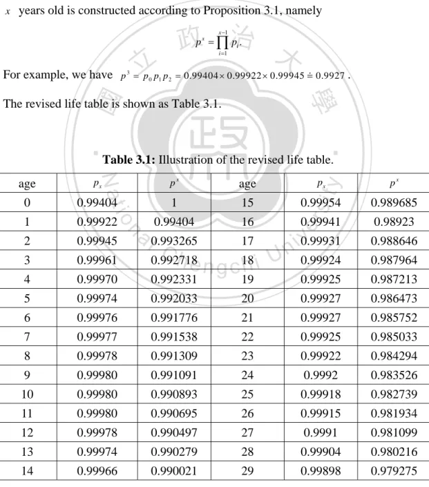
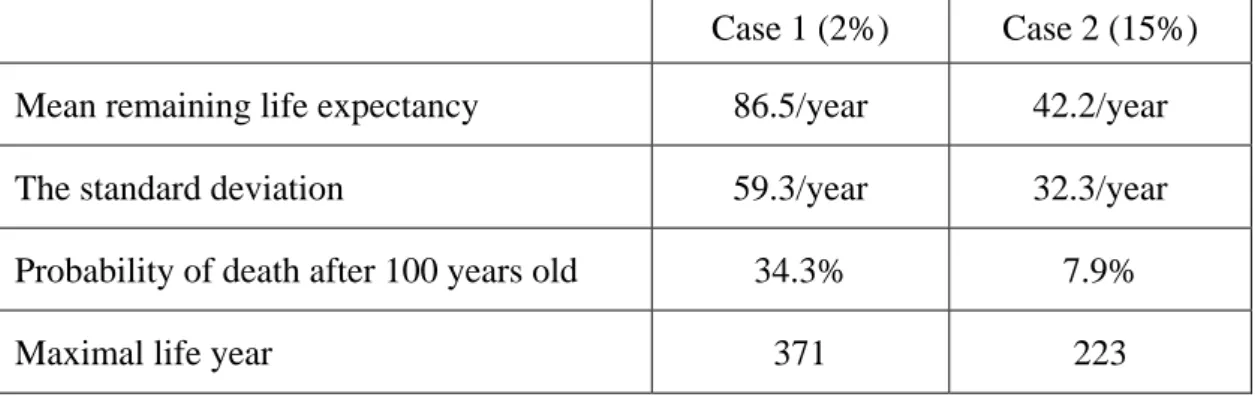
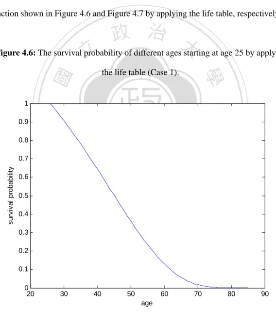
(46) . Case 4: In the transition model of HBV infection in Figure 4.10, assume the probability from “HBeAg(+). HBV-DNA> 2  106~7 IU/ml”. hepatitis. HBV-DNA> 2  104~5 IU/ml”. to. “HBeAg(+) hepatitis. and “HBeAg seroconversion” is 15%.. Example 4.1 Consider scenario (1) with the transition diagram shown in Figure 4.1. First, we compute the probability that a person with initial age s at state i reaches the state j for the first time after n years without applying the life table. Our. 政治大 assume that there is a person who had the chronic hepatitis B virus infection when he 立. computation method is applied as mentioned in Chapter 3. In this example, we. is 25 years old. The original Markov transition matrix is written as follows.. ‧ 國. 學. ‧. 0 0 0 0 0 0 0  0.98 0.013 0.007  0 0.947 0 0 0 0.4 0 0.005 0.008 0   0.05 0 0 0.05 0.9 0 0 0 0 0    0 0 0.82 0.1 0.08 0 0 0 0   0  0 0 0 0.015 0.972 0 0.012 0 0.001 0  . P 0 0 0 0 0.885 0.015 0.04 0.06 0   0  0 0 0 0 0 0 1 0 0 0    0 0 0 0 0 0 0.85 0 0.15  0   0 0 0 0 0 0 0 0.6 0.4   0  0 0 0 0 0 0 0 0 0 1 . n. er. io. sit. y. Nat. al. Hence,. P. Ch. engchi. i n U. v. is a homogeneous matrix since it is time independent.. Then we compute the total probabilities of reaching death and “HBsAg loss” by Theorem 2.3 and equation (2.2.4). More precisely, we can also estimate the probabilities for a person had the chronic hepatitis B virus infection at age 25 at the initially healthy state hits “death” for the first time after n years by equation (2.3.5) and the average transition time from the initially healthy state to death. We show the simulation results as the following Figures 4.2, 4.3, 4.4, 4.5, and Table 4.1. 37 .

(47) . Computing fi ,(mn ) of Case 1 and Case 2.. Let fi,(mn) (25) , n  1, 2, , be the probability of death within one year assuming a patient was aged 25 starting HBV infection. For example, according to equation (3.3.3), we know that fi,(mn) (25) is the probability for an individual who had the HBV infection at age 25 dies when he is exactly at age 25  n . An individual will die eventually, so the sum of the probability of death at different ages is 100%. At first, one individual will not die easily, so the probability of death is small and then increasing year by year. 政治大 age 70, and then the probability decreases since the sum of mortality is 100%. Note 立 because of diseases or accidents. Consider Case 1. The highest mortality is at about. from Figure 4.2 that the corresponding probability is about 0.7% when he is aged 75,. ‧ 國. 學. under the conditions that P1,2  1.3% and P1,3  0.7% .. ‧. sit. y. Nat. Figure 4.2: The mortality of a person who had the HBV infection at age 25 without. 6 probability of death within one year. al. n. x 10. io. -3. 7. er. applying the population mortality rate (Case 1).. Ch. engchi. i n U. v. 5. 4. 3. 2. 1. 0. 0. 50. 100. 150. 200 age. 38 . 250. 300. 350.

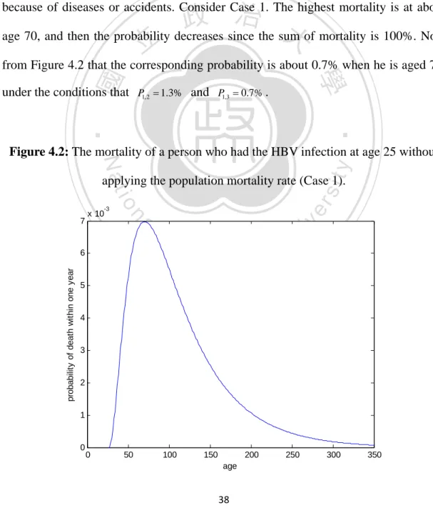
(48) . Figure 4.3: The mortality of a person who had the HBV infection at age 25 without applying the population mortality rate (Case 2).. 0.016. 0.012 0.01 0.008 0.006. 立. 0.004. 0. 50. 100. 150 age. ‧. 0. 政治大. 學. 0.002. ‧ 國. probability of death within one year. 0.014. 250. Nat. y. 200. er. io. sit. Consider Case 2, for example, we know that fi,(mn) (25) is the probability for an individual who had the HBV infection at age 25 dies when he is exactly at age 25  n .. al. n. v i n Ch Note from Figure 4.3 that the corresponding probability for an individual who had the engchi U HBV infection at age 25 dies when he is exactly at the age 52 is about 1.6%, under the conditions that P1,2  10% and P1,3  5% .. 39 .

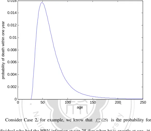
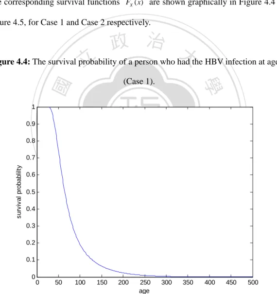
(49) . Computing the survival curves for Case 1 and Case 2.. Naturally assume at initial age for the observed patient the probability of survival is 100%. Then the survival probability decreases year by year eventually approaching to 0%. Note that from equation (3.1.13), the survival function is x t. FX ( x )  1  FX ( x )  1   f i ,(mn ) .. (4.1.1). n 1. The corresponding survival functions FX ( x) are shown graphically in Figure 4.4 and Figure 4.5, for Case 1 and Case 2 respectively.. 政治大 Figure 4.4: The survival probability 立 of a person who had the HBV infection at age 25. 0.9. sit. io. al. n. 0.6. er. 0.7. y. Nat. 0.8. survival probablilty. ‧. ‧ 國. 1. 學. (Case 1).. 0.5. Ch. 0.4. engchi. i n U. v. 0.3 0.2 0.1 0. 0. 50. 100. 150. 200. 250 age. 300. 350. 400. 450. 500. For example, Figure 4.4 shows that the probability for an individual who had the HBV infection at age 25 to survive up to more than 100 years old is about 18%, under the conditions that P1,2  1.3% and P1,3  0.7% . 40 .

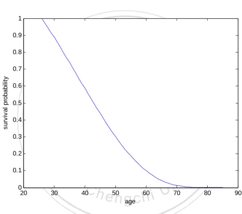
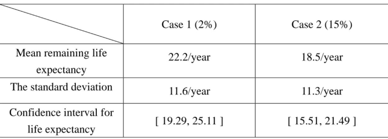
(50) . Figure 4.5: The survival probability of a person who had the HBV infection at age 25 (Case 2).. 1 0.9 0.8. survival probablilty. 0.7 0.6 0.5. 政治大. 0.4. 立. 0.3. 0. 50. 100. 150. 200. 250 age. 300. ‧. 0. 學. 0.1. ‧ 國. 0.2. 350. 400. 500. Nat. sit. y. 450. io. er. Similarly, note from Figure 4.5 that the probability to survive up to more than 100 years old is about 10%, under the conditions that P1,2  10% and P1,3  5% .. n. al. Ch. engchi. i n U. v. Table 4.1 summarizes the mean remaining life expectancy, the standard deviation, probability of death after 100 years old, and the maximal life year. Table 4.1: Summarized results of Case 1 and Case 2 without the life table. Case 1 (2%). Case 2 (15%). Mean remaining life expectancy. 86.5/year. 42.2/year. The standard deviation. 59.3/year. 32.3/year. 34.3%. 7.9%. 371. 223. Probability of death after 100 years old Maximal life year 41 .

(51) . Since the real probability for the transition from “HBeAg(+) hepatitis HBV-DNA> 2  106~7 IU/ml” to “HBeAg(+) hepatitis HBV-DNA> 2  104~5 IU/ml” and “HBeAg(+) hepatitis HBV-DNA> 2  106~7 IU/ml” to “HBeAg seroconversion” are bounded by 2% and 15%. Then, clearly, the real average life expectancy, the standard deviation, the probability of death after 100 years old, and the maximal life year are all bounded by the results of Case 1 and Case 2.. Consider Figure 4.2, Figure 4.3, Figure 4.4, Figure 4.5, and Table 4.1 presented. 政治大 death after 100 years old is 7.9%-34.3% in Case 1 and Case 2 respectively. We found 立 above, it is not difficult to find that the mortality is unreasonable. The probability of. that it is illegitimate for a man or woman staying alive up to almost for 223-371 years. ‧ 國. 學. old. Obviously, it violates the common human expectancy we have known nowadays.. ‧. According to the data from ministry of interior of Taiwan [30], people in Taiwan. sit. y. Nat. usually die before 100 years old. There are only few people in Taiwan who have been. io. er. alive more than one hundred years. Moreover, for a person who had the HBV infection the mean life expectancy is about 42-86 years, which is ever longer than the one who. n. al. Ch. does not get the HBV infection.. engchi. 42 . i n U. v.

(52) . Computing fi ,(mn ) (t ) of Case 1 and Case 2 with the life table.. Now, we conduct the computation by the model proposed in this thesis in Chapter 3. For instance, suppose that there is a person who had the chronic hepatitis B virus infection when he is 25 years old. We calculate the probability that a person with an initial age. t. at the state i reaches the state j for the first time after n years.. Since the initial age is 25, we know that p x  p 25  0.9827 in Table 3.1. For example, we have the one-step transition matrix P 25,26 as follows. By Algorithm 3.1, we know that. 政治大.  p Q P 25,26    0. 立. 25. p 25  R  (1  p 25 )  1 , I . ‧ 國. 學. where Q  M 99 is the transition probability matrix between symptoms, R  M 91 is the transition probability matrix from disease symptoms to death, 1  M 91 is a matrix. ‧. whose elements are all 1, 0  M19 is a zero matrix, and I  M 11 is the identity matrix.. sit. y. Nat. Hence, we have. n. al. er. io. 0 0 0 0 0 0 0.9631 0.0128 0.0069  0 0.9307 0 0 0 0.0393 0 0.0049 0.0079  0.0491 0 0 0.0491 0.8845 0 0 0 0  0 0 0.8058 0.0983 0.0786 0 0 0  0  0 0 0 0.0147 0.9552 0 0.0118 0 0.001  0 0 0 0 0.8697 0.0147 0.0393 0.0590  0  0 0 0 0 0 0 0.9827 0 0  0 0 0 0 0 0 0.8353 0  0  0 0 0 0 0 0 0 0 0.5896   0 0 0 0 0 0 0 0 0. P 25,26. Ch. engchi. i n U. v. 0.0173 0.0173 0.0173  0.0173 0.0173 . 0.0173 0.0173  0.1647   0.4104  1 . The other matrices P k , k 1 can be constructed in the same way for k  25, k   . By applying Theorem 3.3, we obtain fi ,(mn ) (t ) for n   .. 43 .

(53) . Computing the survival curves for Case 1 and Case 2 with the life table.. By equation (3.3.1), (3.3.4) and (4.1.1), we may conduct the computation. The outcomes are displayed in the following Figure 4.6, 4.7 and Table 4.2. Note that equation (4.1.1) is time independent, and the following equation x t. FX ( x ). aged t.  1  FX ( x ) aged t  1   f i ,(mn ) (t ). (4.1.2). n 1. is time dependent. By Theorem 3.3 and equation (4.1.2), we have the survival function shown in Figure 4.6 and Figure 4.7 by applying the life table, respectively.. 政治大 Figure 4.6: The survival 立 probability of different ages starting at age 25 by applying. ‧ 國. y. sit er. al. n. survival probability. io. 0.7. Nat. 0.8. ‧. 0.9. 學. 1. the life table (Case 1).. 0.6 0.5. Ch. engchi. i n U. v. 0.4 0.3 0.2 0.1 0 20. 30. 40. 50. 60 age. 44 . 70. 80. 90.