兩階段工具變數估計量應用於二元反應變數之比較與實證研究 - 政大學術集成

全文

(1)國立政治大學統計學研究所碩士論文. The Performance 政治of Different. 大. Binary Outcomes. 學. ‧ 國. 立 Two-Stage Instrumental Variable Methods for ‧. n. er. io. sit. y. Nat. al. Ch. engchi. i n U. v. 指導教授：江振東博士研究生：莊安婷撰中華民國一百零一年六月.

(2) 謝辭光陰遞嬗，兩年的碩士班生涯即將步入尾聲，論文也在幾陣風雨飄搖中完成。回首來時路，點滴在心頭。撰寫論文期間，面臨不少困難與挫折，但也同時幸運地接受許多幫助，使論文能順利完稿，在此謹以此文表達我無盡的感激與謝意。. 首先，由衷地感謝指導教授－江振東老師的殷殷教誨，讓我在專業知識及待人處事皆有豐盛的收穫。一日為師，終身為父，很高興能成為老師眾多門生的一員。還有，很謝謝口試委員陳珍信老師與杜素豪老師不吝提點，給予許多寶貴的建議，使本篇論文更臻完善。當然，多虧有同窗的陪伴，相互鼓勵打氣，是撰寫. 政治大. 論文時的動力之一，也為這段艱辛的歷程增添不少樂趣。. 立. ‧ 國. 學. 文末，獻上最深的感謝給我的家人－爸爸、媽媽及哥哥，謝謝你們一直以來的陪伴與支持，使我竭力坦然面對所遭遇的一切。欲報之德，昊天罔極！未來，. ‧. 期盼自己能持續懷抱熱情及勇氣，善待周遭的人事物，迎接人生的每一段旅程。. n. er. io. sit. y. Nat. al. Ch. i n U. v. 莊安婷. e n g c h i 壬辰年仲夏書于指南山麓一隅.

(3) 摘要工具變數為處理非隨機試驗所面臨問題的方法之一，近來廣泛應用於計量經濟及流行病學領域；其主要目的在於控制不可觀測的干擾因素，使資料經過調整後「近似」於隨機試驗所得的資料，進而求出處理效果的一致估計值。由於先前研究大多探討連續型變數的情形，本篇論文將透過模擬與實證分析，針對二元之工具變數、反應變數及處理變數，比較一階段廣義線性估計量，two-stage predictor substitution (2SPS)，two-stage residual inclusion (2SRI)，及 two-stage residual inclusion-Taylor expansion (2SRI-T) 這四種估計方法。. 政治大. 模擬結果顯示，當偏誤為主要考量時，2SPS 與 2SRI 有較好的表現；然而，. 立. 同時考慮偏誤及變異的情況下，2SRI-T 則為較適合的估計方法。值得注意的是，. ‧ 國. 學. 模擬試驗所得出的結果與 Terza 等(2008)不同，2SRI 並未優於 2SPS。另外，將此四種方法套用至探討有小孩與否對生活的滿意度的影響之實際資料，其表現結果. ‧. 與模擬試驗結果一致。. n. er. io. sit. y. Nat. al. Ch. engchi. i n U. v.

(4) Abstract Instrumental variable (IV) analysis, one of the techniques to solve problems generated from non-random experiments, has been increasingly applied in many fields such as econometrics and epidemiology. Its utility stems from the belief that IV, if correctly selected, can potentially mimic randomization by adjusting for unmeasured confounders. However, because of less concern about IV analysis on categorical data, we center our discussion on binary outcome, treatment, and IV in this study. Four methods are compared: the one-stage generalized linear model (GLM), two-stage predictor substitution (2SPS), two-stage residual inclusion (2SRI), and. 政治大 the simulation and the empirical 立 study to evaluate the performances of these four. two-stage residual inclusion considering Taylor expansion (2SRI-T). We conduct both. ‧ 國. 學. estimators.. The simulation results indicate that, while 2SPS and 2SRI have better. ‧. performances than the other two estimators with respect to the bias, they suffer from larger variability. On the other hand, 2SRI-T generally has smaller standard error than. Nat. sit. y. 2SPS and 2SRI, and hence might be preferred if MSE is the main concern. Noticeably,. io. er. it also suggests that 2SRI does not outperform 2SPS which was inversely shown in Terza et al. (2008). The same conclusion is also found when implementing these. n. al. Ch. i n U. v. methods on a real dataset to investigate whether having children has significant effect on one’s life satisfaction.. engchi.

(5) Contents 1. Introduction. 1. 2. Statistical Models and Estimation Methods. 5. 2.1 Underlying Assumptions 2.2 IV Methods. 5 5. Simulation and Results. 9. 3. 3.1 Simulation Design 3.2 Results. 治政 Empirical Study and Results 大立 4.1 Data Description Conclusion and Discussion. 24. sit. 22. n. a. er. io. Appendix. Nat. References. ‧. 5. 18 18 21. y. 4.2 Descriptive Analysis 4.3 Results. 18. 學. ‧ 國. 4. 9 11. v. i A: Programming Codel of n CSimulation h e n g c hunder i U Different Values of a B: Histograms of Estimated Coefficients C: Tables of Simulation Results under Different and n D: Questions Used in the WVS Questionnaire in the Empirical Analysis. 26 32 34 44.

(6) Lists of Tables Table 3.1 Table 3.2 Table 3.3. Correlations between D* and Z among Different Values of (a, b) Correlations between D* and C among Different Values of (a, b). 10. Simulation Results as  0 = 0.91 and n = 10,000 under. 14. 11. Smaller Values of a Table 3.4. Simulation Results as  0 = 0.91 and n = 10,000 under. 15. Table 4.1. Larger Values of a Characteristics of Variables Used in the Analysis. 19. Table 4.2. Results of the Four Methods. 立. 政治大. 21. ‧. ‧ 國. 學. n. er. io. sit. y. Nat. al. Ch. engchi. i n U. v.

(7) Lists of Figures Figure 1.1. Diagram for IV and Related Variables. Figure 3.1. Performances of the Four Methods under Fixed a. 12. Figure 3.2. Performances of the Four Methods under Fixed b. 13. 立. 1. 政治大. ‧. ‧ 國. 學. n. er. io. sit. y. Nat. al. Ch. engchi. i n U. v.

(8) Chapter 1 Introduction When discussing causality, randomized experiment is the golden rule to estimate treatment effects and make further inferences. Random assignment of treatments assures nice statistical properties, such as unbiasedness and consistency. However, due to practical or ethical concern, experiment is infeasible sometimes. Take our empirical study provided in Chapter 4 for an example, the primary interest there is the impact of having children on one’s satisfaction towards life, whereas in practice we cannot make a decision of whether to have children for each subject. Therefore, in cases like this, what we obtain is observational data. Under such circumstance, non-random assignment of treatment possibly leads to. 政治大. selection bias. Traditionally, covariate adjustment has been utilized for controlling observable bias. On the other hand, this simultaneously points out the limitation of. 立. covariate adjustment approach- the inability to remove unmeasured confounding,. ‧ 國. 學. which is either unknown or not readily quantifiable. To overcome the difficulty, instrumental variable (IV) analysis provides a viable alternative. By definition, a. ‧. variable, Z, can be called an instrumental variable if it satisfies the following conditions: (1) correlated with the treatment variable; (2) conditionally independent of. y. Nat. sit. the outcome given the treatment variable and all confounders; (3) independent of the. er. io. whole set of immeasurable confounders (Greenland (2000)). Let Y be the outcome. al. n. v i n Crelations a set of measured covariates. The these variables can be illustrated h e n gbetween chi U. variable, D be the treatment variable, C be a set of unmeasured confounders, and X be. as Figure 1.1.. C. Z. Y. D. X Figure 1.1 Diagram for IV and Related Variables. 1.

(9) IV methods rest on the identification of IV to control unmeasured bias, substitution for the actual assignment of treatment, and finally obtaining the estimated treatment effect if all necessary assumptions are met (Angrist et al. (1996), Greene (2003), and Hernán and Robins (2006)). The two-stage least squares (2SLS) approach is the most commonly implemented technique among the IV estimators. The procedures of 2SLS can be formulated as Equations 1.1 and 1.2, the first- and second-stage regression, respectively, where. and. stand for random error terms,. and i and i (i = 0, 1, 2) are the corresponding regression coefficients .. 立. (1.1). 政治大. (1.2). We first find an IV which meets the three conditions stated above and regress the. ‧ 國. 學. treatment on this IV and X (i.e. regress D on Z and X). Then, the observed treatment D is substituted for the predicted value,. , in the second-stage equation for estimation. ‧. of the treatment effect, 1, by regressing Y on. and X . Through this two-step. , a generally biased but consistent estimator of 1. As this. sit. y. Nat. procedure, we can obtain. io. er. method was originated from the field of econometrics, the proof of this nice property can be easily found in many econometrics books (see, for example, Greene (2003),. al. n Kennedy (2003)).. Ch. engchi. i n U. v. Alternatively, Hausman (1978) proposed the two-stage residual inclusion (2SRI) method. The name of the method originated from taking the residual term into account. The first-stage equation of 2SRI is exactly the same as that of 2SLS. However, the second-stage equation is replaced by Equation 1.3.. (1.3) The rationale behind 2SRI approach is that it makes use of. to control. unmeasured confounder C. It looks fine in linear model setting. Indeed, it can be shown that 2SLS and 2SRI yield the same 1 estimate, and hence both methods are consistent. 2.

(10) Obviously, Equations 1.1-1.3 are of a linear model form. For continuous variates, they should work fine. However, as far as categorical treatment variable and/or response variable are concerned, they create a problem.. obtained from either. 2SLS or 2SRI is not consistent any more. Nowadays, IV analysis has been increasingly applied in epidemiology and health services research, in which discrete data are more easily encountered (McClellan et al. (1994), Wang et al. (2005), Brookhart et al. (2006), Schneeweiss et al. (2006), Stukel et al. (2007), Brookhart et al. (2010)). Using IV methods to deal with categorical response and/or treatment variables provides a challenge that researchers need to take on. To overcome inconsistent estimation in the cases of categorical variables, the. 治政 regarded as the rote extension of 2SLS by transforming大 linear models to generalized 立 linear models. With respect to a binary treatment variable D and a binary response Y,. two-stage predictor substitution (2SPS) approach was proposed. In fact, 2SPS can be. ‧ 國. 學. and under the use of logit link function, 2SPS can be stated as Equations 1.4 and 1.5.. ‧. al. (1.5). er. io. .. sit. y. Nat. where. (1.4). n. v i n C h a version of 2SRI In addition, Terza et al. (2008) discussed e n g c h i U to deal with categorical data. Specifically, let. and includes it as an additional. covariate in the second-stage equation, as formulated as Equation 1.6.. (1.6) According to Terza et al. (2008), 2SRI approach is superior to 2SPS under their simulation design in that the estimated treatment effect through 2SRI is consistent. However, we think that, under a nonlinear model setting like Equation 1.4 and 1.5, cannot fully represent C. The finding given in Terza et al. (2008) that favors 2SRI is not sound since their simulated data are constructed so that unmeasured confounders C is of the form of. , that makes their findings in doubt. 3.

(11) In order to provide C a suitable estimate for the estimation of 1, we propose a new version of 2SRI, namely, 2SRI-T. Solving the first-order Taylor expansion term of. for C, 2SRI-T uses it as the role of C in the second stage equation. Due to less concern about IV analysis on categorical data, we center our. discussion on binary outcome, treatment, and IV in this study. The rest of the article is organized as follows. In Chapter 2, related literatures are briefly reviewed and detailed descriptions of 2SLS, 2SPS and 2SRI are provided. In order to compare the performance of 2SLS, 2SPS and 2SRI, a simulation study is performed. Simulation design and results analysis are given in Chapter 3. An empirical study that uses the survey data of the World Value Survey (WVS) in 2005 obtained from Academia. 政治大. Sinica is conducted in Chapter 4. We conclude and discuss the findings in Chapter 5.. 立. ‧. ‧ 國. 學. n. er. io. sit. y. Nat. al. Ch. engchi. 4. i n U. v.

(12) Chapter 2 Statistical Models and Estimation Methods 2.1 Underlying Assumptions Although less known in the statistical literature until recently, the IV method has been well-known and is widely used in the field of economics over fifty years due to the difficulty of conducting controlled experiments. Its utility stems from the belief that IV, if correctly selected, can potentially mimic randomization by adjusting for unmeasured confounders. In contrast, multiple regression with adjusted covariate and propensity score analysis can only adjusted for observable confounders. Let yi, di, zi, xi, and ci denote the outcome, the treatment variable, the instrumental variable, a vector of exogenous covariates, and an unmeasured. 治政大 heavily on the following three assumptions. First, the instrumental variable z is 立 assumed to be associated with d conditional on x . The second assumption is that z is. confounding variable for the ith of n subjects. The usefulness of the IV method hinges i. i. i. i. ‧ 國. 學. uncorrelated with yi conditional on (di, ci, xi). Third, zi is uncorrelated with ci conditional on xi. The second assumption, also called the exclusion restriction,. ‧. indicates that any effect of zi on yi must be via an effect of zi on di. However, this. y. Nat. assumption cannot be verified in that it relates quantities that can never be jointly. sit. observed (Angrist et al. (1996)). The third assumption suggests that zi is uncorrelated. n. al. er. io. with any unmeasured variables which predict yi. That is, no common causes exist. i n U. v. between zi and yi. If this assumption does not hold, zi may relate to yi through an. Ch. engchi. unmeasured confounding variable (Brookhart et al. (2010)). Moreover, Small (2007) pointed out that controlling for xi generally enhances the believability of the second and the third assumption by controlling for variation in unmeasured confounders which is correlated with xi.. 2.2 IV Methods Because our focus in this study is on binary IV, treatment assignment variable, and response, odds ratio is used as the measure of treatment effect to evaluate the performances of different IV methods. With the same focus, Terza et al. (2008) compared the performance of 2SPS and 2SRI methods through a simulation study that we do not quite agree with, and Rassen et al. (2009) exploited IV analysis to address 5.

(13) the similarities and dissimilarities among several IV estimators via three real data sets. In this study, we consider four estimation methods: the traditional one-stage generalized linear model (GLM) that serves as the baseline method to be compared, and three two-stage estimators 2SPS, 2SRI, and 2SRI-T. Their performances will be assessed in terms of simulated data and a real data set. Descriptions of these four approaches are as follows:. (1) One-stage Generalized Linear Models (GLM). (2.1). 政治 is the odds ratio of those who receive 大 the treatment compared to 立 those who do not receive the treatment with observed is the parameter of interest, and. ‧ 國. 學. covariates X controlled. However, this one-stage estimator does not take the unmeasured bias into consideration, and is expected to result in inconsistent .. ‧. estimation of. Nat. n. al. er. io. sit. y. (2) Two-stage Predictor Substitution (2SPS). Ch. engchi. i n U. v. (2.2) (2.3). The 2SPS estimator can be viewed as the extension of the 2SLS method when shifting to the non-linear cases from the linear ones. Equation 2.3 is similar to Equation 2.1, the first stage GLM. What distinguishes the two is that we use the observed value D in Equation 2.1, while in Equation 2.3 it is replaced by the estimates obtained through Equation 2.2.. 6.

(14) (3) Two-stage Residual Inclusion (2SRI). (2.4) (2.5) This is an approach that is consistent with the one introduced by Hausman (1978) for linear models. Similar to 2SPS, the probability of receiving the treatment is estimated by Equation 2.4. Instead of plugging replace D,. into the second stage equation to. is calculated and plugged in to replace C.. According to Terza et al. (2008), in fully linear models, the 2SLS method is. 政治大 nonlinear case. Hence, there is a need to compare their performances under nonlinear 立 model settings.. identical to 2SPS and 2SRI approaches. However, they yield different outcomes in the. ‧ 國. 學. (4) Two-stage Residual Inclusion- Taylor Expansion (2SRI-T). ‧. n. al. where r and M are known nonlinear functions.. Ch. engchi. (2.7). er. io. sit. y. Nat. (2.6). i n U. v. The framework considered in Terza et al. (2008) is as above. Because of the way unmeasured confounder C is defined, it is legitimate to substitute C in the first equation by . And a consistent 2SRI estimator is expected. However, the functional form of Equation 2.6 associated with D is not quite the same as the one we previously discussed, that is, (2.8) Since their simulated data also constructed using Equation 2.6, this makes their findings that 2SRI yields consistent estimates and its performance is much better than that of 2SPS questionable. In order to find a proper estimate of C in terms of Equation 2.8, we propose the following approach based on the first-order Taylor expansion term of 7. . Let r be the.

(15) expit function. Note that. , it follows that. , and hence. This prompts us to consider play the role as. , to. 政治大. in Equation 2.5. And we term the approach as 2SRI-T.. Specifically, this method is formulated as follows:. 立. ‧. ‧ 國. 學. n. er. io. sit. y. Nat. al. Ch. engchi. 8. i n U. v. (2.9) (2.10).

(16) Chapter 3 Simulation and Results 3.1 Simulation Design To explore the properties of the IV estimators delineated in the previous section, we conducted a simulation study. The study design was similar to that of Johnston et al. (2008). As binary outcome was of the primary interest, data were simulated for a Bernoulli-distributed response variable. Different levels of correlation between the treatment and the instrument, and between the treatment and unobserved confounder were considered. The simulation procedure was carried out as follows: 1. Generate an unobserved confounder (C) from a standard normal distribution,. 治政大 standard normal Let Z* be a latent variable generated from an independent 立 distribution, and let Z be a binary instrumental variable generated from Z* such N(0,1), and a covariate X from N( 2, 42).. 學. that. ‧ 國. 2.. .. ‧. 3. Generate the latent variable D*= aZ+bC+X+ , where a and b indicate the. y. Nat. is. sit. strengths of IV and confounding effect associated with D*, respectively, and. al. n. treatment (D) so that. er. io. an error term from an independent standard normal distribution. Define the. Ch. engchi. i n .U. v. 4. Generate the outcome variable Y from a Bernoulli distribution with the logit of the probability of response equal to  0  log(3) D  log(0.5)C  log(0.75) X , that is, the odds ratio associated with D, C and X are 3, 0.5, and 0.75, respectively. 5. Estimate the odds ratio associated with D by fitting a traditional generalized linear model (GLM) with a logit link without accounting for C, and by fitting 2SPS and 2SRI with logit links. Two versions of residual are considered in 2SRI method, namely, C  D  exp it( 0  1Z   2 X ) , and. C. D  expit( 0  1Z   2 X ) . [expit( 0  1Z   2 X )  (1  expit( 0  1Z   2 X ))] 9.

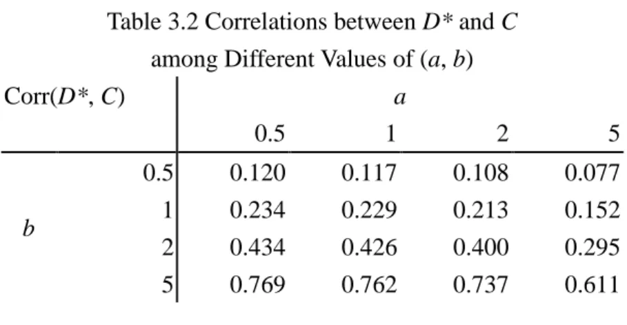
(17) In step 3, 0.5, 1, 2, 5 were considered for a and b, respectively. There were altogether 16 combinations. Tables 3.1 and 3.2 displayed the corresponding correlation coefficients of D* and Z, and D* and C, respectively. Formulas for the calculations are as follows. Since D*= aZ+bC+X+ , it follows that Cov( D* , Z ). Corr( D* , Z ) . Var( D* ) Var( Z ) Cov( aZ  bC  , Z ) Var(aZ  bC  ) Var( Z ). . a  Var( Z ). . a 2 Var( Z )  b 2 Var(C )  Var( ) Var( Z ) a. . 立. Cov(aZ  bC  , C ) Var(aZ  bC  ) Var(C ) b  Var(C ). io. a 2 Var( Z )  b 2 Var(C )  Var( ) Var(C ). n. abl. er. . ‧. Var( D* ) Var(C ). Nat. . Cov( D* , C ). y. Corr( D* , C ) . 學. ‧ 國. a 2  b 2  17. sit. . Similarly,. 政治大. a  b 2  17 1 a 2.  . Ch. a 2  b 2  17 1 b. engchi. i n U. v. a 2  b 2  17. Table 3.1 Correlations between D* and Z among Different Values of (a, b) a Corr(D*, Z). b. 0.5 1 2 5. 0.5. 1. 2. 5. 0.120 0.117 0.108 0.077. 0.234 0.229 0.213 0.152. 0.434 0.426 0.400 0.295. 0.769 0.762 0.737 0.611. 10.

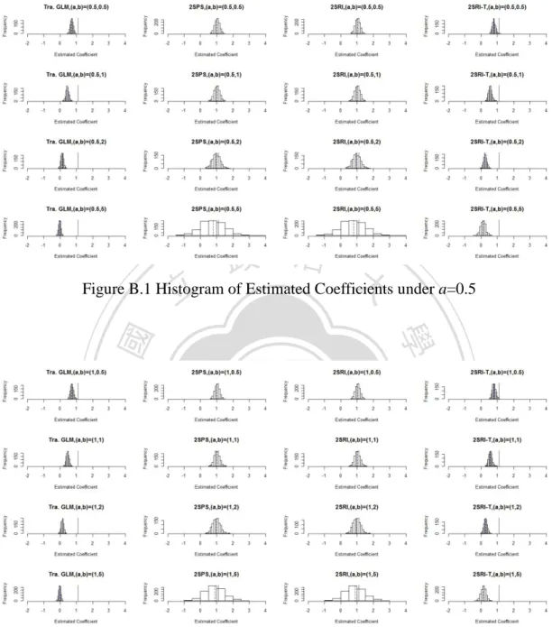
(18) Table 3.2 Correlations between D* and C among Different Values of (a, b) a 0.5 1 2. Corr(D*, C). 0.5 1 2 5. b. 0.120 0.234 0.434 0.769. 0.117 0.229 0.426 0.762. 5. 0.108 0.213 0.400 0.737. 0.077 0.152 0.295 0.611. As shown in the two tables, stronger association between D* and Z corresponds to larger a and smaller b, while stronger association between D* and C relates to both larger a and larger b. More specifically, with the increasing value of a and the fixed. 政治大. value of b, we can see from Tables 3.1 and 3.2 that Corr(D*, Z) levels up and. 立. Corr(D*, C) levels down. However, although the values of Corr(D*, C) are declining,. ‧ 國. 學. their values are roughly the same, indicating that the changing the value of a influences more on the strength of IV. By the same argument, with the increasing. ‧. value of b and the fixed value of a, it results in a decrease in Corr(D*, Z) and an increase in Corr(D*, C). However, changing the value of b appears to influence more. y. Nat. sit. on the strength of confounding effect.. er. io. Subsequently, in step 4, three levels of  0 were considered: 0, 0.91, and 3, which corresponds to 0.50, 0.71, and 0.95 for P(Y  1| Z  C  X  0) . In addition,. al. n. v i n the sample sizes n considered were For each combination of a, b, C h1,000 and 10,000. U i e h n forc1,000 iterations. Bias, standard error,  , and n, the above steps were carried outg 0. mean squared error (MSE), and coverage probability of the estimated coefficients were calculated to evaluate the performance of the methods. The programming code is provided in Appendix A. 3.2 Results Since the results were basically the same regardless of the value of  0 and the sample size n, our discussion focused only on the case with  0 = 0.91 and n = 10,000. We hence presented only the information associated with  0 = 0.91 and n = 10,000 in Figures 3.1 and 3.2, and Tables 3.3 and 3.4 (As for the histograms of the estimated coefficients, please refer to Appendix B.). The simulation results for the rest of 11.

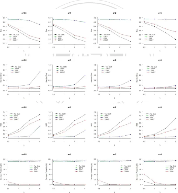
(19) combinations of  0 and n were tabulated in Appendix C. Most strikingly, we found that 2SRI did not outperform 2SPS which was inversely shown in Terza et al. (2008). The two indeed had almost the same performance. Generally speaking, when 2SPS and 2SRI had better performances than the other two estimators with respect to the bias, they suffered from larger variability. On the other hand, 2SRI-T generally had smaller standard error than 2SPS and 2SRI, and hence might be preferred if MSE was the main concern. Detailed comparisons from the perspective of bias, standard error, MSE, and coverage probability for the four estimators were given in the following subsections.. 立. 政治大. ‧. ‧ 國. 學. n. er. io. sit. y. Nat. al. Ch. engchi. i n U. v. Figure 3.1 Performances of the Four Methods under Fixed a. 12.

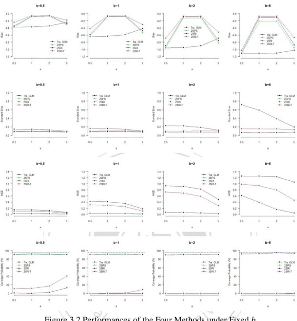
(20) 立. 政治大. ‧. ‧ 國. 學. n. er. io. sit. y. Nat. al. Ch. i n U. v. Figure 3.2 Performances of the Four Methods under Fixed b. engchi. 13.

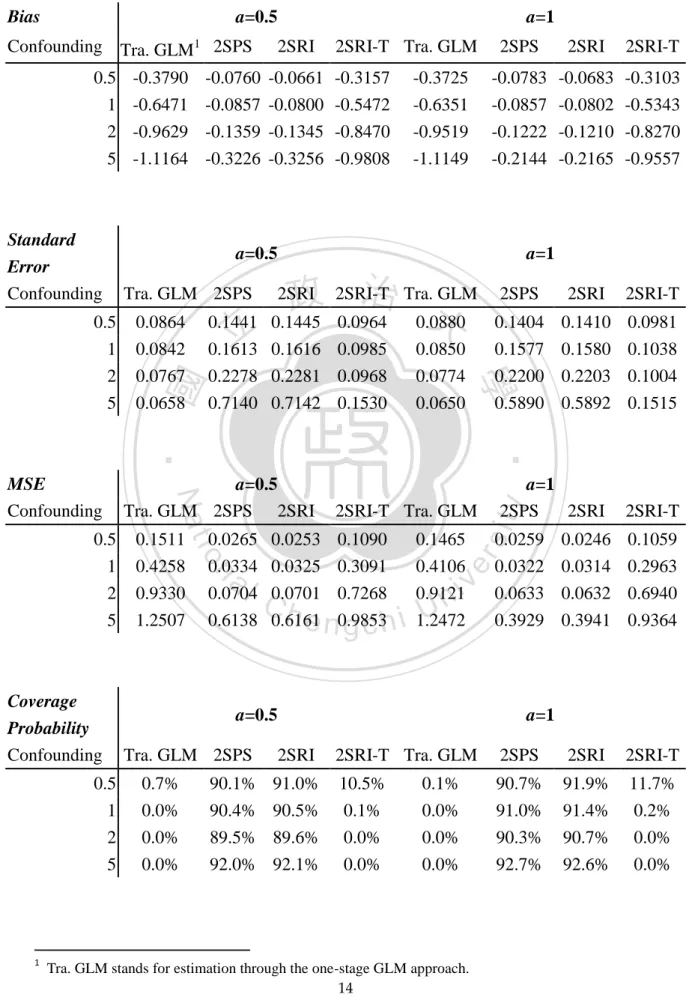
(21) Table 3.3 Simulation Results as  0 = 0.91 and n = 10,000 under Weaker IV Bias. a=0.5. Confounding Tra. GLM1 2SPS 0.5 1 2 5. Standard Error Confounding. -0.0760 -0.0857 -0.1359 -0.3226. 2SRI -0.0661 -0.0800 -0.1345 -0.3256. 2SRI-T Tra. GLM -0.3157 -0.5472 -0.8470 -0.9808. -0.3725 -0.6351 -0.9519 -1.1149. 2SPS. 2SRI. 2SRI-T. -0.0783 -0.0857 -0.1222 -0.2144. -0.0683 -0.0802 -0.1210 -0.2165. -0.3103 -0.5343 -0.8270 -0.9557. 2SPS. 2SRI. 2SRI-T. 0.1404 0.1577 0.2200 0.5890. 0.1410 0.1580 0.2203 0.5892. 0.0981 0.1038 0.1004 0.1515. a=0.5. 0.0265 0.0334 0.0704 0.6138. al. n. Coverage Probability Confounding. 0.1511 0.4258 0.9330 1.2507. io. 0.5 1 2 5. Nat. a=0.5 Tra. GLM 2SPS 2SRI 0.0253 0.0325 0.0701 0.6161. Ch. 0.0964 0.0985 0.0968 0.1530. 0.0880 0.0850 0.0774 0.0650. 2SRI-T Tra. GLM. y. 0.1445 0.1616 0.2281 0.7142. ‧. ‧ 國. 立. a=1 2SPS 2SRI. 2SRI-T. 0.1090 0.3091 0.7268 0.9853. 0.0259 0.0322 0.0633 0.3929. 0.0246 0.0314 0.0632 0.3941. 0.1059 0.2963 0.6940 0.9364. engchi. 0.1465 0.4106 0.9121 1.2472. sit. 0.1441 0.1613 0.2278 0.7140. 治 Tra. GLM 政 2SRI-T 大. 2SRI. 學. MSE Confounding. 0.0864 0.0842 0.0767 0.0658. a=1. er. Tra. GLM 2SPS. 0.5 1 2 5. 1. -0.3790 -0.6471 -0.9629 -1.1164. a=1. i n U. v. a=0.5 Tra. GLM 2SPS. 2SRI. a=1 2SRI-T Tra. GLM. 2SPS. 2SRI. 2SRI-T. 0.5. 0.7%. 90.1% 91.0%. 10.5%. 0.1%. 90.7%. 91.9%. 11.7%. 1 2 5. 0.0% 0.0% 0.0%. 90.4% 90.5% 89.5% 89.6% 92.0% 92.1%. 0.1% 0.0% 0.0%. 0.0% 0.0% 0.0%. 91.0% 90.3% 92.7%. 91.4% 90.7% 92.6%. 0.2% 0.0% 0.0%. Tra. GLM stands for estimation through the one-stage GLM approach. 14.

(22) Table 3.4 Simulation Results as  0 = 0.91 and n = 10,000 under Stronger IV. -0.3441 -0.5915 -0.9041 -1.1055. -0.0764 -0.0766 -0.0925 -0.1071. Standard. -0.2432 -0.4170 -0.6920 -1.0247. -0.0616 -0.0639 -0.0749 -0.0764. -0.0586 -0.0623 -0.0749 -0.0771. -0.1821 -0.3097 -0.5214 -0.6679. 2SPS. 2SRI. 2SRI-T. 0.0952 0.1016 0.1202 0.1922. 0.0955 0.1018 0.1203 0.1922. 0.0880 0.0947 0.1012 0.1312. 0.1272 0.1410 0.1857 0.1859 0.1048 0.3860 0.3862 0.1485. 0.1260 0.3574 0.8235 1.2267. 0.0752 0.0707. ‧. a=2 2SPS 2SRI. 2SRI-T Tra. GLM. 0.0220 0.0258 0.0431 0.1605. 0.0889 0.2456 0.5873 0.7920. al. 0.0208 0.0252 0.0430 0.1608. Ch. engchi. 0.0652 0.1800 0.4846 1.0550. a=5 2SPS 2SRI. 2SRI-T. 0.0129 0.0144 0.0201 0.0428. 0.0125 0.0142 0.0201 0.0429. 0.0409 0.1049 0.2821 0.4633. y. Tra. GLM. 2SRI-T Tra. GLM. 治 0.0779 政 0.0995 0.1276 大 0.1413 0.1047 0.0786. 立. 2SRI-T. a=5 2SRI. n. Coverage Probability Confounding. 0.0873 0.0868 0.0777 0.0668. 2SPS. io. 0.5 1 2 5. Tra. GLM. Nat. MSE Confounding. -0.2812 -0.4844 -0.7592 -0.8775. 學. 0.5 1 2 5. 2SRI-T Tra. GLM. a=2. ‧ 國. Error Confounding. -0.0672 -0.0721 -0.0918 -0.1083. a=5 2SPS 2SRI. sit. 0.5 1 2 5. Tra. GLM. a=2 2SPS 2SRI. er. Bias Confounding. i n U. v. a=2. a=5. Tra. GLM. 2SPS. 2SRI. 2SRI-T Tra. GLM. 2SPS. 2SRI. 2SRI-T. 0.5. 2.3%. 90.8%. 91.4%. 16.8%. 12.8%. 90.1%. 90.6%. 40.5%. 1 2 5. 0.0% 0.0% 0.0%. 91.1% 91.2% 94.6%. 91.4% 91.2% 94.7%. 0.7% 0.0% 0.0%. 0.1% 0.0% 0.0%. 90.4% 90.7% 93.2%. 90.5% 90.7% 93.1%. 8.6% 0.0% 0.2%. 15.

(23) 3.2.1 Bias Moving from the top to the bottom of each column in Tables 3.3 and 3.4, since changing the value of b impact more on Corr(D*, C), we can see that biases increase as confounding levels up no matter the value of a and estimators that are considered. This finding goes along well with our expectation. On the other hand, for the three two-stage estimators, as we go from the left to the right of the table, suggesting the increase of Corr(D*, Z), we can also find that biases are decreasing. This, too, is as expected. Although we can also find that the one-stage GLM estimator also shares the same finding that biases are decreasing as a goes up, it should be noted that the changes are not due to the increase of Corr(D*, Z), but the decrease of Corr(D*, C), as. 治政大 that IV really does its diminishes as the effect of IV becomes stronger, it suggests 立 work. Among the four estimators, the one-stage GLM estimator is outperformed by the one-stage GLM estimator has nothing to do with IV. Since the amount of bias. ‧ 國. 學. the other three two-stage estimators in each (a, b) setting. 2SPS and 2SRI have similar performances with smaller biases than 2SRI-T method.. ‧ y. Nat. 3.2.2 Standard Error. sit. Intuitively, we may think that the more serious confounding, the more variation. n. al. er. io. of the estimator. In the three two-stage estimators, it is really this case as we can see. i n U. v. from the top to the bottom of each column in Tables 3.3 and 3.4. However, the. Ch. engchi. standard error of the one-stage GLM estimator slightly declines as confounding becomes more serious. Besides, as a increases while holding on the level of b, the three two-stage estimators become less varied, whereas the one-stage GLM method does not share the same pattern. Among the four estimators, the one-stage GLM approach has the smallest standard error, ranging from 0.06 to 0.09, 2SRI-T has the second smallest ones, falling between 0.08 and 0.15, while the standard errors of 2SPS and 2SRI range from 0.09 to 0.71, and vary the most.. 16.

(24) 3.2.3 MSE As an index to evaluate estimators, MSE simultaneously takes bias and standard error into consideration. Hence, an estimator with small MSE represents both small bias and small variability. Generally speaking, when confounding becomes more serious, MSEs of all the four estimators augment. It is also true that the values of MSE decline as IV grows in strength. Overall, the three two-stage estimators had smaller MSEs than the one-stage GLM estimator. Moreover, 2SPS and 2SRI, again similarly performed, generally outperform 2SRI-T in terms of MSE. However, we do observe situations where 2SRI-T might have better performances than 2SPS and 2SRI particularly when the smaller biases, that they usually have, cannot offset the effect of. 政治大. large variability.. 立3.2.4 Coverage Probability. ‧ 國. 學. Set the desired value of 0.95, the coverage probabilities of 2SPS and 2SRI are quite close to it, while that of 2SRI-T and the one-stage GLM estimators are far from. ‧. it. It makes sense since the latter two estimators generally result in larger biases,. y. Nat. which result in confidence intervals easier to miss the mark. Although having poor. sit. performances, 2SRI-T is still superior to the one-stage GLM estimator. Generally. n. al. er. io. speaking, the coverage probabilities of these two relative poor methods reduced as. i n U. v. confounding levels up. As for 2SPS and 2SRI, there is no big difference between the two.. Ch. engchi. 17.

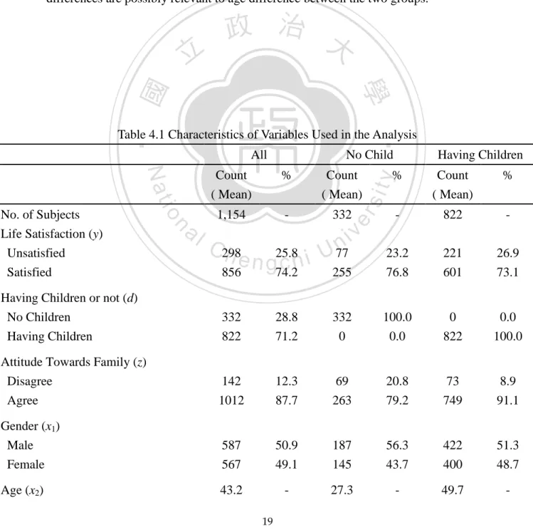
(25) Chapter 4 Empirical Study and Results 4.1 Data Description To empirically compare the performance of 2SPS, 2SRI, and 2SRI-T to an observational data set, we consider the data coming from the World Value Survey (WVS), a worldwide survey conducted once every five years since 1981 in Europe. We use the part of Taiwan data collected in 2005. This particular survey includes many realms of questions, ranging from oneself, interpersonal relationship, family to society, environment, culture, and global issues. There are 253 questions in total. The number of subjects completed the survey successfully is 1,227. Our primary interest in this study is the effect of having children on one’s life. 政治大. satisfaction. In the past, most researchers utilized covariates adjustment method, i.e., the traditional one-step GLM model, to remove potential confounding in a study like. 立. this. However, as delineated in Chapter 1, one of the problems associated with this. ‧ 國. 學. method is the inability to control unmeasured bias. And this is why IV comes into play. We choose the attitude towards family, a question that asks subjects whether or not. the IV.. ‧. they agree a child can only grow up with happiness in a family with both parents, as. y. Nat. sit. To sum up, the outcome (y) is whether or not one is satisfied with his/her life,. er. io. the treatment (d) is whether one has children or not, and the IV (z) asks one’s opinion. al. n. v i n settings discussed in Chapter 3. C In h addition, we consider e n g c h i U another nine variables. in family. All these three are binary variables, exactly the same as the simulation. serving as the control covariates. Corresponding to all variables used in our analysis, the related questions in the WVS survey is provided in Appendix D. After the data cleaning process, the sample size involved in this study is 1,154. Descriptive statistics of the variables and subsequent analyses are provided in the following sections.. 4.2 Descriptive Analysis Table 4.1 displays the characteristics of all variables used in this study with respect to the whole sample, those who have no child, and those with children. The nine control covariates (x1, …, x9) encompass one’s basic information, such as gender, age, levels of education, economic status, and so on. 18.

(26) Among 1,154 subjects, 332 have no child and 822 are having children. As can be seen from the table, there exist obvious differences between those with no child and those having children in six of the nine control variates- age, family income class, primary breadwinner, economic status, social class, and education level. Generally speaking, those with no child are younger, having higher family income, less primary breadwinner, with more saving, with higher social class, and more educated. With respect to the IV, attitude towards family, their distributions are roughly the same, but for those without children, they slightly more disagree that children can only grow up with happiness in a family with both parents present. However, we suspect that the differences are possibly relevant to age difference between the two groups.. 立. 政治大. ‧ 國. 學 %. %. ( Mean). io. 1,154. -. n. C298 h e n g25.8 chi. 332. er. ( Mean). al. Count. sit. Count. No Child. y. All. Nat No. of Subjects Life Satisfaction (y) Unsatisfied Satisfied. ‧. Table 4.1 Characteristics of Variables Used in the Analysis. i n U 77. v. Having Children Count. %. ( Mean) -. 822. -. 221 601. 26.9 73.1. 856. 74.2. 255. 23.2 76.8. 332 822. 28.8 71.2. 332 0. 100.0 0.0. 0 822. 0.0 100.0. Disagree Agree. 142 1012. 12.3 87.7. 69 263. 20.8 79.2. 73 749. 8.9 91.1. Gender (x1) Male Female. 587 567. 50.9 49.1. 187 145. 56.3 43.7. 422 400. 51.3 48.7. Age (x2). 43.2. -. 27.3. -. 49.7. -. Having Children or not (d) No Children Having Children Attitude Towards Family (z). 19.

(27) Race (x3) 939 97. 81.4 8.4. 269 33. 81.0 9.9. 670 64. 81.5 7.8. 97. 8.4. 27. 8.1. 70. 8.5. 21. 1.8. 3. 0.9. 18. 2.2. Family Income Class (x4) Low Medium High. 339 779 36. 29.4 67.5 3.1. 55 266 11. 16.6 80.1 3.3. 284 513 25. 34.5 62.4 3.0. Primary Breadwinner (x5) No Yes. 648 506. 56.2 43.8. 233. 70.2 29.8. 415 407. 50.5 49.5. 329 478 220 127. 28.5 41.4 19.1 11.0. 113 128 60 31. 34.0 38.6 18.1 9.3. 216 350 160 96. 26.3 42.6 19.5 11.7. 308. 26.7. 95. 28.6. 213. 25.9. 416 359 71. 36.0 31.1 6.2. 151 76 10. 45.5 22.9 3.0. 265 283 61. 32.2 34.4 7.4. Education Level (x9) Middle School or Lower High School College or Above. al. n. Employment Status (x8) Unemployed Employed. Ch. engchi. y. sit. io. Lower Middle Working Class Lower Class. Nat. Social Class (x7) Above Upper Middle. ‧. ‧ 國. 立. 學. Economic Status (x6) Saving Even Spending Some Savings Spending Savings and Borrowing. 政治大99. er. Minnan from Taiwan Hakka from Taiwan Mainlander from Any City or Province Others. i n U. v. 372 782. 32.2 67.8. 86 246. 25.9 74.1. 286 536. 34.8 65.2. 378 332. 32.8 28.7. 28 84. 8.4 25.3. 350 248. 42.6 30.2. 444. 38.5. 220. 66.3. 224. 27.3. 20.

(28) 4.3 Results We analyze the data by implementing each method discussed in Chapter 3: one-stage GLM, 2SPS, 2SRI, and 2SRI-T. We intend to investigate the effect of having children on life satisfaction, and compare the results of the four different approaches. Moreover, we examine the validity of IV, i.e., attitude towards family, used in the three two-step estimators by a GLM with logit link, where the dependent variable is the treatment (d) and the regressors are the IV (z) and the nine control covariates. We first examine the validity of the IV through the first stage regression model in the two-step procedures. It indicates that a significant association between d and z. 治政大 2, whereas the other two example does meet the first assumption described in Chapter 立 assumptions cannot be verified in that we have no information about the unmeasured is found, with p-value = 0.03, suggesting that this IV is valid. Hence, the IV in our. ‧ 國. 學. confounders. In addition, we also find the relationship between one’s opinion in family and the life satisfaction is not that strong.. ‧. Table 4.2 presents the empirical results of the four estimators. Although a. y. Nat. consistent finding that whether or not having children does not have significant effect. sit. on one’s life satisfaction is reached at significance level   0.05 no matter which. n. al. er. io. approach is utilized, the estimates are apparently somewhat different. Again, we. i n U. v. observe that 2SPS and 2SRI perform similarly, with similar estimated values and. Ch. engchi. standard errors. On the other hand, the traditional one-stage GLM and 2SRI-T are less varied than 2SPS and 2SRI.. Table 4.2 Results of the Four Methods Estimate Standard Error Tra. GLM 2SPS 2SRI 2SRI-T. 0.192 -0.042 -0.084 0.425. 0.394 0.507 0.869 0.291. 21. p-value 0.225 0.934 0.509 0.144.

(29) Chapter 5 Conclusion and Discussion In the previous two chapters, we conducted both simulation and the empirical studies to evaluate the performances of different IV estimators when applied in analyzing data sets with binary outcome, treatment, and IV. In addition to the traditional one-stage GLM, 2SPS, and 2SRI, we also consider 2SRI-T, a version of 2SRI that intends to replace unmeasured confounders through the use of the first-order Taylor expansion term of the error term. D. . In the simulation design,. strengths of IV, levels of confounding, probabilities of receiving the treatment, and sample sizes were considered in altogether 16 combined scenarios. Bias, standard error, MSE, and coverage probability are the main tools to evaluate the performances. 治政大 data from Survey one’s life satisfaction in the empirical study, using the WVS 立 Research Data Archive of Center for Survey Research, Academia Sinica.. of the four estimators. Subsequently, we investigated the effect of having children on. ‧ 國. 學. Contradictory to Terza et al. (2008), we found that 2SRI did not outperform 2SPS according to the simulation results. In fact, these two had almost the same. ‧. performances. As far as bias is concerned, 2SPS and 2SRI outperformed the other two. y. Nat. estimators, and the one-stage GLM had the worst performance. Somewhat beyond our. sit. expectation was that 2SRI-T did not perform as well as 2SRI. On the other hand,. n. al. er. io. 2SPS and 2SRI suffered from larger variability, while 2SRI-T generally had smaller. i n U. v. standard error. Therefore, 2SRI-T might be preferred if MSE was the main concern.. Ch. engchi. As for the empirical study, the results revealed that having children or not did not significantly impact one’s life satisfaction. The conclusion was agreed upon no matter which method was applied. Moreover, the results of the four approaches were consistent with what we observed in the simulation study. 2SPS and 2SRI again had similar performances with similar estimated treatment effect and standard error, and standard errors were larger than the other two estimators. Before concluding this chapter, we need to emphasize that the usefulness of the results we provide in this study rests on the availability of an appropriate IV. However, this is also a problem associated with any IV analysis. Without an appropriate IV, any of the methods cannot be implemented. Furthermore, due to the binary nature of the variables, we focus only on odds ratio as the effect of treatment. However, in many 22.

(30) studies, risk difference and risk ratio may also be the parameters of interest. It may be worthwhile to investigate the performance of these IV estimators on the estimation of risk difference and risk ratio as well.. 立. 政治大. ‧. ‧ 國. 學. n. er. io. sit. y. Nat. al. Ch. engchi. 23. i n U. v.

(31) References 1. Angrist JD, Imbens G, Rubin DB. Identification of causal effects using instrumental variables. Journal of the American Statistical Association. 1996; 94(434): 444-455. 2. Brookhart MA, Wang PS, Solomon DH, Schneeweiss S. Evaluating short-term drug effects using a physical-specific prescribing preference as an instrumental variable. Epidemiology. 2006; 17(3): 268-275. 3. Brookhart MA, Rassen JA, Schneeweiss S. Instrumental variable methods in comparative safety and effectiveness research. Pharmacoepidemiology and Drug Safety.2010; 19(6): 537-554. 4. Greene WH. Econometric Analysis. 5th ed. Upper Saddle, River, NJ: Prentice Hall; 2003. 5. Greenland S. An introduction to instrumental variables for epidemiologists. International Journal of Epidemiology. 2000; 29: 722-729.. 立. 政治大. ‧. ‧ 國. 學. 6. Hausman JA. Specification tests in econometrics. Econometrica. 1978; 46:1251-1271. 7. Hernán MA, Robins JM. Instruments for causal inference: an epidemiologist’s dream? Epidemiology. 2006; 17(4): 360-372. 8. Johnston KM, Gustafson P, Levy AR, Grootendorst P. Use of instrumental variables in the analysis of generalized linear models in the presence. y. Nat. sit. n. al. er. io. of unmeasured confounding with applications to epidemiological research. Statistics in Medicine. 2008;27: 1539-1556. 9. Kennedy P. A guide to Econometrics. 5th ed. Cambridge, MA: MIT Press; 2003. 10. McClellan M, McNeil BJ, Newhouse JP. Does more intensive treatment of acute myocardial infarction in the elderly reduce mortality? Analysis using instrumental variables. Journal of the American Medical Association. 1994; 272(11): 859-866. 11. Rassen JA, Schneeweiss S, Glynn RJ, Mittleman MA, Brookhart MA. Instrumental variable analysis for estimation of treatment effects with dichotomous outcomes. American Journal of Epidemiology. 2009; 169(3):273-284. 12. Schneeweiss S, Solomon DH, Wang PS, Rassen JA, Brookhart MA. Simultaneous. Ch. engchi. i n U. v. assessment of short-term gastrointestinal benefits and cardiovascular risks of selective cyclooxygenase 2 inhibitors and nonselective nonsteroidal antiinflammatory drugs: an instrumental variable analysis. Arthritis Rheumatism. 2006; 54(11): 3390-3398.. 24.

(32) 13. Small DS. Sensitivity analysis for instrumental variables regression with overidentifying restrictions. Journal of the American Statistical Association. 2007; 102(479): 1049-1058. 14. Stukel TA, Fisher ES, Wennberg DE, Alter DA, Gottlieb DJ, Vermeulen MJ. Analysis of observational studies in the presence of treatment selection bias: effects of invasive cardiac management on AMI survival using propensity score and instrumental variable methods. Journal of the American Medical Association. 2007; 297(3): 444-455. 15. Terza JV, Basu A, Rathouz PJ. Two-stage Residual inclusion estimation: addressing endogeneity in health econometric modeling. Journal of Health Economics. 2008; 27(3): 531-543. 16. Wang PS, Schneeweiss S, Avorn J, Fiescher MA, Mogun H, Solomon DH, Brookhart MA. Risk of death in elderly users of conventional vs. atypical antipsychotic medications. New England Journal of Medicine. 2005; 353(22): 2335-2341.. 立. 政治大. ‧. ‧ 國. 學. n. er. io. sit. y. Nat. al. Ch. engchi. 25. i n U. v.

(33) Appendix A. Programming Code of Simulation (Under a=0.5,  0 =0.91, and n=10,000) a=.5; b1=.5; b2=1; b3=2; b4=5 n=10000. temp.tra.or.1=NULL;temp.sps.or.1=NULL;temp.sri.or.1=NULL;temp.tay.or.1=NULL temp.tra.or.2=NULL;temp.sps.or.2=NULL;temp.sri.or.2=NULL;temp.tay.or.2=NULL temp.tra.or.3=NULL;temp.sps.or.3=NULL;temp.sri.or.3=NULL;temp.tay.or.3=NULL temp.tra.or.4=NULL;temp.sps.or.4=NULL;temp.sri.or.4=NULL;temp.tay.or.4=NULL. for (i in 1:1000){ set.seed(591208+117*i) Z.=rnorm(n,0,1). 立. set.seed(139084+315*i) C=rnorm(n,0,1). 政治大. ‧ 國. 學. set.seed(92843+131*i) e=rnorm(n,0,1). Nat. Z=ifelse(Z.>0,1,0). y. X=rnorm(n,-2,4). ‧. set.seed(240789+117*i). sit. D1.=a*Z+b1*C+X+e; D2.=a*Z+b2*C+X+e; D3.=a*Z+b3*C+X+e; D4.=a*Z+b4*C+X+e. n. al. er. io. D1=ifelse(D1. > 0, 1, 0); D2=ifelse(D2. > 0, 1, 0); D3=ifelse(D3. > 0, 1, 0); D4=ifelse(D4. > 0, 1, 0). Ch. i n U. lambda1=as.vector(numeric(n)); lambda2=as.vector(numeric(n)). engchi. lambda3=as.vector(numeric(n)); lambda4=as.vector(numeric(n)) p1=as.vector(numeric(n)); p2=as.vector(numeric(n)) p3=as.vector(numeric(n)); p4=as.vector(numeric(n)) y1=as.vector(numeric(n)); y2=as.vector(numeric(n)) y3=as.vector(numeric(n)); y4=as.vector(numeric(n)). int=log(411/166) for (j in 1:n){ lambda1[j]=int+log(3)*D1[j]+log(.5)*C[j]+log(.75)*X[j] lambda2[j]=int+log(3)*D2[j]+log(.5)*C[j]+log(.75)*X[j] lambda3[j]=int+log(3)*D3[j]+log(.5)*C[j]+log(.75)*X[j] lambda4[j]=int+log(3)*D4[j]+log(.5)*C[j]+log(.75)*X[j]. 26. v.

(34) p1[j]=exp(lambda1[j])/(1+exp(lambda1[j])); p2[j]=exp(lambda2[j])/(1+exp(lambda2[j])) p3[j]=exp(lambda3[j])/(1+exp(lambda3[j])); p4[j]=exp(lambda4[j])/(1+exp(lambda4[j])) set.seed(327043+100*j-104) y1[j]=rbinom(1,1,p1[j]) set.seed(327043+100*j-104) y2[j]=rbinom(1,1,p2[j]) set.seed(327043+100*j-104) y3[j]=rbinom(1,1,p3[j]) set.seed(327043+100*j-104) y4[j]=rbinom(1,1,p4[j]) }. data.mat.1=cbind(y1,D1,Z,X) fst.ols.1=lm(D1~Z+X). 立. 政治大. fst.glm.1=glm(D1~Z+X,data=data.frame(data.mat.1),family=binomial(link=logit)) D1.glm.hat=fst.glm.1$fitted.values. ‧ 國. 學. D1.ols.hat=fst.ols.1$fitted.values D1.new=D1.glm.hat-D1. ‧. D1.tay= (D1-D1.glm.hat)/(D1.glm.hat*(1-D1.glm.hat)). y. Nat. tra.or.1=glm(y1~D1+X,data=data.frame(data.mat.1),family=binomial(link=logit)). sit. sps.or.1=glm(y1~D1.glm.hat+X,data=data.frame(data.mat.1),family=binomial(link=logit)). al. er. io. sri.or.1=glm(y1~D1+X+D1.new,data=data.frame(data.mat.1),family=binomial(link=logit)). v. n. tay.or.1=glm(y1~D1+X+D1.tay,data=data.frame(data.mat.1),family=binomial(link=logit)). data.mat.2=cbind(y2,D2,Z,X). Ch. engchi. i n U. fst.ols.2=lm(D2~Z+X) fst.glm.2=glm(D2~Z+X,data=data.frame(data.mat.2),family=binomial(link=logit)) D2.glm.hat=fst.glm.2$fitted.values D2.ols.hat=fst.ols.2$fitted.values D2.new=D2.glm.hat-D2 D2.tay= (D2-D2.glm.hat)/(D2.glm.hat*(1-D2.glm.hat)). tra.or.2=glm(y2~D2+X,data=data.frame(data.mat.2),family=binomial(link=logit)) sps.or.2=glm(y2~D2.glm.hat+X,data=data.frame(data.mat.2),family=binomial(link=logit)) sri.or.2=glm(y2~D2+X+D2.new,data=data.frame(data.mat.2),family=binomial(link=logit)) tay.or.2=glm(y2~D2+X+D2.tay,data=data.frame(data.mat.2),family=binomial(link=logit)). 27.

(35) data.mat.3=cbind(y3,D3,Z,X) fst.ols.3=lm(D3~Z+X) fst.glm.3=glm(D3~Z+X,data=data.frame(data.mat.3),family=binomial(link=logit)) D3.glm.hat=fst.glm.3$fitted.values D3.ols.hat=fst.ols.3$fitted.values D3.new=D3.glm.hat-D3 D3.tay= (D3-D3.glm.hat)/(D3.glm.hat*(1-D3.glm.hat)). tra.or.3=glm(y3~D3+X,data=data.frame(data.mat.3),family=binomial(link=logit)) sps.or.3=glm(y3~D3.glm.hat+X,data=data.frame(data.mat.3),family=binomial(link=logit)) sri.or.3=glm(y3~D3+X+D3.new,data=data.frame(data.mat.3),family=binomial(link=logit)) tay.or.3=glm(y3~D3+X+D3.tay,data=data.frame(data.mat.3),family=binomial(link=logit)). data.mat.4=cbind(y4,D4,Z,X). 立. fst.ols.4=lm(D4~Z+X). 政治大. fst.glm.4=glm(D4~Z+X,data=data.frame(data.mat.4),family=binomial(link=logit)). ‧ 國. 學. D4.glm.hat=fst.glm.4$fitted.values D4.ols.hat=fst.ols.4$fitted.values. ‧. D4.new=D4.glm.hat-D4. D4.tay= (D4-D4.glm.hat)/(D4.glm.hat*(1-D4.glm.hat)). y. Nat. sit. tra.or.4=glm(y4~D4+X,data=data.frame(data.mat.4),family=binomial(link=logit)). al. er. io. sps.or.4=glm(y4~D4.glm.hat+X,data=data.frame(data.mat.4),family=binomial(link=logit)). v. n. sri.or.4=glm(y4~D4+X+D4.new,data=data.frame(data.mat.4),family=binomial(link=logit)). Ch. i n U. tay.or.4=glm(y4~D4+X+D4.tay,data=data.frame(data.mat.4),family=binomial(link=logit)). engchi. temp.tra.or.1=c(temp.tra.or.1,summary(tra.or.1)$coefficients[2],summary(tra.or.1)$coefficients[5]) temp.sps.or.1=c(temp.sps.or.1,summary(sps.or.1)$coefficients[2],summary(sps.or.1)$coefficients[5]) temp.sri.or.1=c(temp.sri.or.1,summary(sri.or.1)$coefficients[2],summary(sri.or.1)$coefficients[6]) temp.tay.or.1=c(temp.tay.or.1,summary(tay.or.1)$coefficients[2],summary(tay.or.1)$coefficients[6]) temp.tra.or.2=c(temp.tra.or.2,summary(tra.or.2)$coefficients[2],summary(tra.or.2)$coefficients[5]) temp.sps.or.2=c(temp.sps.or.2,summary(sps.or.2)$coefficients[2],summary(sps.or.2)$coefficients[5]) temp.sri.or.2=c(temp.sri.or.2,summary(sri.or.2)$coefficients[2],summary(sri.or.2)$coefficients[6]) temp.tay.or.2=c(temp.tay.or.2,summary(tay.or.2)$coefficients[2],summary(tay.or.2)$coefficients[6]) temp.tra.or.3=c(temp.tra.or.3,summary(tra.or.3)$coefficients[2],summary(tra.or.3)$coefficients[5]) temp.sps.or.3=c(temp.sps.or.3,summary(sps.or.3)$coefficients[2],summary(sps.or.3)$coefficients[5]) temp.sri.or.3=c(temp.sri.or.3,summary(sri.or.3)$coefficients[2],summary(sri.or.3)$coefficients[6]) temp.tay.or.3=c(temp.tay.or.3,summary(tay.or.3)$coefficients[2],summary(tay.or.3)$coefficients[6]) 28.

(36) temp.tra.or.4=c(temp.tra.or.4,summary(tra.or.4)$coefficients[2],summary(tra.or.4)$coefficients[5]) temp.sps.or.4=c(temp.sps.or.4,summary(sps.or.4)$coefficients[2],summary(sps.or.4)$coefficients[5]) temp.sri.or.4=c(temp.sri.or.4,summary(sri.or.4)$coefficients[2],summary(sri.or.4)$coefficients[6]) temp.tay.or.4=c(temp.tay.or.4,summary(tay.or.4)$coefficients[2],summary(tay.or.4)$coefficients[6]) }. #Form Coefficients and Their Standard Errors as Matrices# tra.or.coef.1=matrix(temp.tra.or.1,2,1000);sps.or.coef.1=matrix(temp.sps.or.1,2,1000);sri.or.coef.1=mat rix(temp.sri.or.1,2,1000);tay.or.coef.1=matrix(temp.tay.or.1,2,1000) tra.or.coef.2=matrix(temp.tra.or.2,2,1000);sps.or.coef.2=matrix(temp.sps.or.2,2,1000);sri.or.coef.2=mat rix(temp.sri.or.2,2,1000);tay.or.coef.2=matrix(temp.tay.or.2,2,1000) tra.or.coef.3=matrix(temp.tra.or.3,2,1000);sps.or.coef.3=matrix(temp.sps.or.3,2,1000);sri.or.coef.3=mat rix(temp.sri.or.3,2,1000);tay.or.coef.3=matrix(temp.tay.or.3,2,1000). 政治大. tra.or.coef.4=matrix(temp.tra.or.4,2,1000);sps.or.coef.4=matrix(temp.sps.or.4,2,1000);sri.or.coef.4=mat. 立. rix(temp.sri.or.4,2,1000);tay.or.coef.4=matrix(temp.tay.or.4,2,1000). ‧ 國. 學. data.or=rbind(tra.or.coef.1,sps.or.coef.1,sri.or.coef.1,tay.or.coef.1,tra.or.coef.2,sps.or.coef.2,sri.or.coef.2 ,tay.or.coef.2,tra.or.coef.3,sps.or.coef.3,sri.or.coef.3,tay.or.coef.3,tra.or.coef.4,sps.or.coef.4,sri.or.coef.4,t. ‧. ay.or.coef.4). rownames(data.or)=c("beta.tra.1","se.tra.1","beta.sps.1","se.sps.1","beta.sri.1","se.sri.1","beta.tay.1","s. y. Nat. e.tay.1","beta.tra.2","se.tra.2","beta.sps.2","se.sps.2","beta.sri.2","se.sri.2","beta.tay.2","se.tay.2","beta.t. sit. ra.3","se.tra.3","beta.sps.3","se.sps.3","beta.sri.3","se.sri.3","beta.tay.3","se.tay.3","beta.tra.4","se.tra.4". ##Calculate bias##. er. al. n. data1.or=t(data.or). io. ,"beta.sps.4","se.sps.4","beta.sri.4","se.sri.4","beta.tay.4","se.tay.4"). Ch. engchi. i n U. v. bias.tra.or.1 = mean(tra.or.coef.1[1,])-log(3); bias.sps.or.1 = mean(sps.or.coef.1[1,])-log(3) bias.sri.or.1 = mean(sri.or.coef.1[1,])-log(3); bias.tay.or.1 = mean(tay.or.coef.1[1,])-log(3) bias.tra.or.2 = mean(tra.or.coef.2[1,])-log(3); bias.sps.or.2 = mean(sps.or.coef.2[1,])-log(3) bias.sri.or.2 = mean(sri.or.coef.2[1,])-log(3); bias.tay.or.2 = mean(tay.or.coef.2[1,])-log(3) bias.tra.or.3 = mean(tra.or.coef.3[1,])-log(3); bias.sps.or.3 = mean(sps.or.coef.3[1,])-log(3) bias.sri.or.3 = mean(sri.or.coef.3[1,])-log(3); bias.tay.or.3 = mean(tay.or.coef.3[1,])-log(3) bias.tra.or.4 = mean(tra.or.coef.4[1,])-log(3); bias.sps.or.4 = mean(sps.or.coef.4[1,])-log(3) bias.sri.or.4 = mean(sri.or.coef.4[1,])-log(3); bias.tay.or.4 = mean(tay.or.coef.4[1,])-log(3) bias.or=matrix(c(bias.tra.or.1,bias.sps.or.1,bias.sri.or.1,bias.tay.or.1,bias.tra.or.2,bias.sps.or.2,bias.sri.or. 2,bias.tay.or.2,bias.tra.or.3,bias.sps.or.3,bias.sri.or.3,bias.tay.or.3,bias.tra.or.4,bias.sps.or.4,bias.sri.or.4,b ias.tay.or.4),nrow=4,ncol=4,byrow=T) colnames(bias.or)=c("Tra. GLM","2SPS","2SRI-L","2SRI-T"); rownames(bias.or)=c(0.5,1,2,5) 29.

(37) ##Calculate standard error## se.tra.or.1 = sd(tra.or.coef.1[1,]); se.sps.or.1 = sd(sps.or.coef.1[1,]) se.sri.or.1 = sd(sri.or.coef.1[1,]); se.tay.or.1 = sd(tay.or.coef.1[1,]) se.tra.or.2 = sd(tra.or.coef.2[1,]); se.sps.or.2 = sd(sps.or.coef.2[1,]) se.sri.or.2 = sd(sri.or.coef.2[1,]); se.tay.or.2 = sd(tay.or.coef.2[1,]) se.tra.or.3 = sd(tra.or.coef.3[1,]); se.sps.or.3 = sd(sps.or.coef.3[1,]) se.sri.or.3 = sd(sri.or.coef.3[1,]); se.tay.or.3 = sd(tay.or.coef.3[1,]) se.tra.or.4 = sd(tra.or.coef.4[1,]); se.sps.or.4 = sd(sps.or.coef.4[1,]) se.sri.or.4 = sd(sri.or.coef.4[1,]); se.tay.or.4 = sd(tay.or.coef.4[1,]). se.or=matrix(c(se.tra.or.1,se.sps.or.1,se.sri.or.1,se.tay.or.1,se.tra.or.2,se.sps.or.2,se.sri.or.2,se.tay.or.2,se.t ra.or.3,se.sps.or.3,se.sri.or.3,se.tay.or.3,se.tra.or.4,se.sps.or.4,se.sri.or.4,se.tay.or.4),nrow=4,ncol=4,byro w=T). 政治大. colnames(se.or)=colnames(bias.or); rownames(se.or)=rownames(bias.or). 立. mse.tra.or.1 = var(tra.or.coef.1[1,])+ mean(tra.or.coef.1[1,]-log(3))^2 mse.sps.or.1 = var(sps.or.coef.1[1,])+ mean(sps.or.coef.1[1,]-log(3))^2. 學. ‧ 國. #Calculate MSE##. ‧. mse.sri.or.1 = var(sri.or.coef.1[1,])+ mean(sri.or.coef.1[1,]-log(3))^2 mse.tay.or.1 = var(tay.or.coef.1[1,])+ mean(tay.or.coef.1[1,]-log(3))^2. al. n. mse.tay.or.2 = var(tay.or.coef.2[1,])+ mean(tay.or.coef.2[1,]-log(3))^2. Ch. er. io. mse.sri.or.2 = var(sri.or.coef.2[1,])+ mean(sri.or.coef.2[1,]-log(3))^2. i n U. mse.tra.or.3 = var(tra.or.coef.3[1,])+ mean(tra.or.coef.3[1,]-log(3))^2. engchi. y. mse.sps.or.2 = var(sps.or.coef.2[1,])+ mean(sps.or.coef.2[1,]-log(3))^2. sit. Nat. mse.tra.or.2 = var(tra.or.coef.2[1,])+ mean(tra.or.coef.2[1,]-log(3))^2. v. mse.sps.or.3 = var(sps.or.coef.3[1,])+ mean(sps.or.coef.3[1,]-log(3))^2 mse.sri.or.3 = var(sri.or.coef.3[1,])+ mean(sri.or.coef.3[1,]-log(3))^2 mse.tay.or.3 = var(tay.or.coef.3[1,])+ mean(tay.or.coef.3[1,]-log(3))^2 mse.tra.or.4 = var(tra.or.coef.4[1,])+ mean(tra.or.coef.4[1,]-log(3))^2. mse.sps.or.4 = var(sps.or.coef.4[1,])+ mean(sps.or.coef.4[1,]-log(3))^2 mse.sri.or.4 = var(sri.or.coef.4[1,])+ mean(sri.or.coef.4[1,]-log(3))^2 mse.tay.or.4 = var(tay.or.coef.4[1,])+ mean(tay.or.coef.4[1,]-log(3))^2. mse.or=matrix(c(mse.tra.or.1,mse.sps.or.1,mse.sri.or.1,mse.tay.or.1,mse.tra.or.2,mse.sps.or.2,mse.sri.or. 2,mse.tay.or.2,mse.tra.or.3,mse.sps.or.3,mse.sri.or.3,mse.tay.or.3,mse.tra.or.4,mse.sps.or.4,mse.sri.or.4, mse.tay.or.4),nrow=4,ncol=4,byrow=T) colnames(mse.or)=colnames(bias.or); rownames(mse.or)=rownames(bias.or). 30.

(38) ##Calculate Coverage Probability## cp.tra.or.1 = sum( tra.or.coef.1[1,]+1.96*tra.or.coef.1[2,] >= log(3) & tra.or.coef.1[1,]-1.96*tra.or.coef.1[2,] <= log(3) )/1000 cp.sps.or.1 = sum( sps.or.coef.1[1,]+1.96*sps.or.coef.1[2,] >= log(3) & sps.or.coef.1[1,]-1.96*sps.or.coef.1[2,] <= log(3) )/1000 cp.sri.or.1 = sum( sri.or.coef.1[1,]+1.96*sri.or.coef.1[2,] >= log(3) & sri.or.coef.1[1,]-1.96*sri.or.coef.1[2,] <= log(3) )/1000 cp.tay.or.1 = sum( tay.or.coef.1[1,]+1.96*tay.or.coef.1[2,] >= log(3) & tay.or.coef.1[1,]-1.96*tay.or.coef.1[2,] <= log(3) )/1000 cp.tra.or.2 = sum( tra.or.coef.2[1,]+1.96*tra.or.coef.2[2,] >= log(3) & tra.or.coef.2[1,]-1.96*tra.or.coef.2[2,] <= log(3) )/1000 cp.sps.or.2 = sum( sps.or.coef.2[1,]+1.96*sps.or.coef.2[2,] >= log(3) & sps.or.coef.2[1,]-1.96*sps.or.coef.2[2,] <= log(3) )/1000. 政治大. cp.sri.or.2 = sum( sri.or.coef.2[1,]+1.96*sri.or.coef.2[2,] >= log(3) &. 立. sri.or.coef.2[1,]-1.96*sri.or.coef.2[2,] <= log(3) )/1000. cp.tay.or.2 = sum( tay.or.coef.2[1,]+1.96*tay.or.coef.2[2,] >= log(3) &. ‧ 國. 學. tay.or.coef.2[1,]-1.96*tay.or.coef.2[2,] <= log(3) )/1000 cp.tra.or.3 = sum( tra.or.coef.3[1,]+1.96*tra.or.coef.3[2,] >= log(3) &. ‧. tra.or.coef.3[1,]-1.96*tra.or.coef.3[2,] <= log(3) )/1000 cp.sps.or.3 = sum( sps.or.coef.3[1,]+1.96*sps.or.coef.3[2,] >= log(3) &. y. Nat. sps.or.coef.3[1,]-1.96*sps.or.coef.3[2,] <= log(3) )/1000. sit. cp.sri.or.3 = sum( sri.or.coef.3[1,]+1.96*sri.or.coef.3[2,] >= log(3) &. al. n. cp.tay.or.3 = sum( tay.or.coef.3[1,]+1.96*tay.or.coef.3[2,] >= log(3) &. Ch. tay.or.coef.3[1,]-1.96*tay.or.coef.3[2,] <= log(3) )/1000. engchi. er. io. sri.or.coef.3[1,]-1.96*sri.or.coef.3[2,] <= log(3) )/1000. i n U. v. cp.tra.or.4 = sum( tra.or.coef.4[1,]+1.96*tra.or.coef.4[2,] >= log(3) & tra.or.coef.4[1,]-1.96*tra.or.coef.4[2,] <= log(3) )/1000. cp.sps.or.4 = sum( sps.or.coef.4[1,]+1.96*sps.or.coef.4[2,] >= log(3) & sps.or.coef.4[1,]-1.96*sps.or.coef.4[2,] <= log(3) )/1000 cp.sri.or.4 = sum( sri.or.coef.4[1,]+1.96*sri.or.coef.4[2,] >= log(3) & sri.or.coef.4[1,]-1.96*sri.or.coef.4[2,] <= log(3) )/1000 cp.tay.or.4 = sum( tay.or.coef.4[1,]+1.96*tay.or.coef.4[2,] >= log(3) & tay.or.coef.4[1,]-1.96*tay.or.coef.4[2,] <= log(3) )/1000. cp.or=matrix(c(cp.tra.or.1,cp.sps.or.1,cp.sri.or.1,cp.tay.or.1,cp.tra.or.2,cp.sps.or.2,cp.sri.or.2,cp.tay.or.2,c p.tra.or.3,cp.sps.or.3,cp.sri.or.3,cp.tay.or.3,cp.tra.or.4,cp.sps.or.4,cp.sri.or.4,cp.tay.or.4),nrow=4,ncol=4, byrow=T) colnames(cp.or)=colnames(bias.or); rownames(cp.or)=rownames(bias.or) 31.

(39) Appendix B. Histograms of Estimated Coefficients under Different Values of a. 政治大 Figure B.1 Histogram of Estimated Coefficients under a=0.5 立 ‧. ‧ 國. 學. n. er. io. sit. y. Nat. al. Ch. engchi. i n U. v. Figure B.2 Histogram of Estimated Coefficients under a=1. 32.

(40) 政治大. Figure B.3 Histogram of Estimated Coefficients under a=2. 立. ‧. ‧ 國. 學. n. er. io. sit. y. Nat. al. Ch. engchi. i n U. v. Figure B.4 Histogram of Estimated Coefficients under a=5. 33.

(41) Appendix C. Tables of Simulation Results under Different  0 and n Table C.1.1 Simulation Results as  0 = 0.71 and n = 1,000 under Weaker IV Bias Confounding. a=0.5 a=1 Tra. GLM 2SPS-L 2SRI-L 2SRI-T Tra. GLM 2SPS-L 2SRI-L 2SRI-T. 0.5 1 2 5 SE Confounding. -0.4090 -0.6699 -0.9636 -1.1086. -0.1012 -0.1107 -0.1466 -0.2206. -0.0921 -0.1058 -0.1464 -0.2264. -0.3067 -0.5113 -0.8031 -1.0412. -0.4064 -0.6568 -0.9546 -1.1067. -0.1040 -0.1102 -0.1346 -0.1508. -0.0946 -0.1049 -0.1336 -0.1533. -0.3020 -0.4935 -0.7838 -1.0053. a=0.5 a=1 Tra. GLM 2SPS-L 2SRI-L 2SRI-T Tra. GLM 2SPS-L 2SRI-L 2SRI-T 0.4434. 1 2 5. 0.2541 0.2271 0.1939. 0.5042 0.7045 2.2006. MSE Confounding. ‧ 國. 0.2634. 治 0.2646 政 0.3409 大 0.5048 0.3257 0.2608. 立. 0.4447. 0.4308. 0.4324. 0.3316. 0.7052 2.2053. 0.4891 0.6728 1.9100. 0.4899 0.6733 1.9126. 0.3350 0.3248 0.5056. 0.3215 0.5058. 0.2309 0.1945. 學. 0.5. ‧. a=0.5 a=1 Tra. GLM 2SPS-L 2SRI-L 2SRI-T Tra. GLM 2SPS-L 2SRI-L 2SRI-T 0.2063. 0.2103. 0.2352. 1 2 5. 0.5133 0.9801 1.2667. 0.2664 0.5178 4.8912. 0.2660 0.5187 4.9147. 0.3675 0.7483 1.3399. 0.4995 0.9647 1.2627. n. Ch. a=0.5. engchi. er. io. Coverage Probability Confounding. al. 0.1964. y. 0.2069. sit. 0.2367. Nat. 0.5. i n U. v. 0.2514 0.4708 3.6707. 0.1959. 0.2011. 0.2510 0.4712 3.6815. 0.3558 0.7199 1.2663. a=1. Tra. GLM 2SPS-L 2SRI-L 2SRI-T Tra. GLM 2SPS-L 2SRI-L 2SRI-T. 0.5 1 2. 65.9% 24.9% 1.4%. 93.8% 93.6% 92.9%. 93.9% 93.7% 92.7%. 82.7% 61.2% 26.7%. 65.5% 29.1% 1.7%. 94.0% 93.9% 93.1%. 94.2% 93.7% 93.1%. 83.0% 62.2% 30.1%. 5. 0.0%. 93.4%. 93.6%. 45.7%. 0.0%. 93.8%. 93.8%. 47.5%. 34.

(42) Table C.1.2 Simulation Results as  0 = 0.71 and n = 1,000 under Stronger IV Bias a=2 a=5 Confounding Tra. GLM 2SPS-L 2SRI-L 2SRI-T Tra. GLM 2SPS-L 2SRI-L 2SRI-T 0.5 1 2 5. -0.3775 -0.6137 -0.9097 -1.0990. -0.1086 -0.1096 -0.1243 -0.0892. -0.0987 -0.1044 -0.1227 -0.0890. -0.2670 -0.4416 -0.7133 -0.9099. -0.2868 -0.4508 -0.7121 -1.0247. -0.1083 -0.1120 -0.1225 -0.1072. -0.1049 -0.1104 -0.1228 -0.1081. -0.1815 -0.2694 -0.4704 -0.6415. SE a=2 a=5 Confounding Tra. GLM 2SPS-L 2SRI-L 2SRI-T Tra. GLM 2SPS-L 2SRI-L 2SRI-T 0.5 1 2. 0.2619 0.2562 0.2340. 0.3889 0.4351 0.5690. 5. 0.1979. 1.2574. 0.3191 0.3201 0.3286. 0.2417 0.2418 0.2343. 政治大 1.2588 0.4853 0.2108. 0.2995 0.3188 0.3670. 0.3002 0.3191 0.3676. 0.2971 0.3033 0.3101. 0.5847. 0.5854. 0.3986. 學. ‧ 國. 立. 0.3901 0.4359 0.5701. MSE a=2 a=5 Confounding Tra. GLM 2SPS-L 2SRI-L 2SRI-T Tra. GLM 2SPS-L 2SRI-L 2SRI-T 0.1731 0.2975 0.6167. 0.1406 0.2617 0.5620. 5. 1.2471. 1.5890. 1.5926. 1.0633. 1.0944. 0.3534. 0.1011 0.1141 0.1502. 0.1212 0.1646 0.3175. 0.3544. 0.5704. er. io. al. 0.1014 0.1142 0.1497. y. 0.1619 0.2009 0.3401. sit. 0.1630 0.2013 0.3392. ‧. 0.2111 0.4422 0.8823. Nat. 0.5 1 2. v. n. Coverage a=2 a=5 Probability Confounding Tra. GLM 2SPS-L 2SRI-L 2SRI-T Tra. GLM 2SPS-L 2SRI-L 2SRI-T 0.5 1 2 5. 67.6% 32.1% 2.8% 0.0%. 94.1% 93.6% 93.3% 94.2%. Ch. engchi. 94.0% 93.5% 93.1% 94.1%. 85.4% 65.8% 35.5% 48.2%. 35. i n U. 77.3% 51.7% 13.9% 0.1%. 93.9% 93.7% 94.8% 95.6%. 94.2% 93.8% 94.8% 95.6%. 89.1% 80.6% 69.1% 55.5%.

(43) Table C.2.1 Simulation Results as  0 = 0 and n = 1,000 under Weaker IV Bias a=0.5 a=1 Confounding Tra. GLM 2SPS-L 2SRI-L 2SRI-T Tra. GLM 2SPS-L 2SRI-L 2SRI-T 0.5 1 2 5. -0.4284 -0.6677 -0.9528 -1.0998. -0.1473 -0.1480 -0.1486 -0.1199. -0.1413 -0.1438 -0.1482 -0.1274. -0.3306 -0.5116 -0.7891 -0.9751. -0.4302 -0.6600 -0.9431 -1.0985. -0.1497 -0.1529 -0.1485 -0.0945. -0.1432 -0.1483 -0.1477 -0.0985. -0.3331 -0.5092 -0.7750 -0.9495. SE a=0.5 a=1 Confounding Tra. GLM 2SPS-L 2SRI-L 2SRI-T Tra. GLM 2SPS-L 2SRI-L 2SRI-T 0.5 1 2. 0.2233 0.2156 0.1979. 0.3523 0.3975 0.5606. 5. 0.1687. 1.7763. 0.2754 0.2834 0.2800. 0.2179 0.2129 0.1931. 政治大 1.7766 0.4248 0.1680. 0.3449 0.3876 0.5358. 0.3464 0.3882 0.5363. 0.2763 0.2751 0.2764. 1.5615. 1.5620. 0.4267. 學. ‧ 國. 立. 0.3540 0.3982 0.5612. MSE a=0.5 a=1 Confounding Tra. GLM 2SPS-L 2SRI-L 2SRI-T Tra. GLM 2SPS-L 2SRI-L 2SRI-T 0.1852 0.3420 0.7010. 0.2325 0.4809 0.9267. 5. 1.2380. 3.1695. 3.1725. 1.1313. 1.2349. 2.4472. 0.1405 0.1727 0.3094. 0.1873 0.3349 0.6771. 2.4497. 1.0837. er. io. al. 0.1414 0.1736 0.3091. y. 0.1453 0.1793 0.3369. sit. 0.1458 0.1799 0.3364. ‧. 0.2334 0.4923 0.9471. Nat. 0.5 1 2. v. n. Coverage a=0.5 a=1 Probability Confounding Tra. GLM 2SPS-L 2SRI-L 2SRI-T Tra. GLM 2SPS-L 2SRI-L 2SRI-T 0.5 1 2 5. 50.0% 12.9% 0.3% 0.0%. 92.2% 92.5% 93.4% 93.6%. Ch. engchi. 92.0% 92.7% 93.4% 93.6%. 73.6% 47.3% 18.1% 32.4%. 36. i n U. 49.3% 13.0% 0.2% 0.0%. 92.0% 92.4% 93.2% 94.1%. 92.1% 92.4% 93.3% 94.1%. 74.6% 48.9% 17.8% 35.2%.

(44) Table C.2.2 Simulation Results as  0 = 0 and n = 1,000 under Stronger IV Bias a=2 a=5 Confounding Tra. GLM 2SPS-L 2SRI-L 2SRI-T Tra. GLM 2SPS-L 2SRI-L 2SRI-T 0.5 1 2 5. -0.4070 -0.6249 -0.9008 -1.0872. -0.1607 -0.1559 -0.1376 -0.0755. -0.1532 -0.1514 -0.1361 -0.0764. -0.3107 -0.4745 -0.7124 -0.8623. -0.3132 -0.4620 -0.7031 -1.0084. -0.1568 -0.1499 -0.1299 -0.0974. -0.1515 -0.1470 -0.1287 -0.0966. -0.2110 -0.2956 -0.4637 -0.6393. SE a=2 a=5 Confounding Tra. GLM 2SPS-L 2SRI-L 2SRI-T Tra. GLM 2SPS-L 2SRI-L 2SRI-T 0.5 1 2. 0.2092 0.2050 0.1941. 0.3186 0.3526 0.4605. 5. 0.1666. 1.0349. 0.2617 0.2632 0.2719. 0.1893 0.1898 0.1843. 政治大 1.0357 0.4027 0.1695. 0.2408 0.2534 0.2926. 0.2413 0.2536 0.2929. 0.2310 0.2414 0.2582. 0.4730. 0.4735. 0.3185. 學. ‧ 國. 立. 0.3195 0.3533 0.4610. MSE a=2 a=5 Confounding Tra. GLM 2SPS-L 2SRI-L 2SRI-T Tra. GLM 2SPS-L 2SRI-L 2SRI-T 0.1650 0.2944 0.5815. 0.1340 0.2495 0.5283. 5. 1.2098. 1.0768. 1.0786. 0.9057. 1.0456. 0.2332. 0.0812 0.0859 0.1023. 0.0979 0.1457 0.2816. 0.2336. 0.5102. er. io. al. 0.0826 0.0867 0.1025. y. 0.1256 0.1477 0.2310. sit. 0.1273 0.1486 0.2310. ‧. 0.2094 0.4326 0.8492. Nat. 0.5 1 2. v. n. Coverage a=2 a=5 Probability Confounding Tra. GLM 2SPS-L 2SRI-L 2SRI-T Tra. GLM 2SPS-L 2SRI-L 2SRI-T 0.5 1 2 5. 52.0% 15.0% 0.5% 0.0%. 91.4% 92.1% 93.7% 95.1%. Ch. engchi. 91.8% 92.2% 93.8% 95.1%. 76.4% 52.4% 21.1% 40.8%. 37. i n U. 63.3% 31.7% 3.6% 0.0%. 89.6% 90.6% 92.0% 94.4%. 90.1% 90.9% 92.0% 94.4%. 82.9% 70.7% 46.0% 41.3%.

(45) Table C.3.1 Simulation Results as  0 = 0 and n = 10,000 under Weaker IV Bias Confounding. a=0.5 a=1 Tra. GLM 2SPS-L 2SRI-L 2SRI-T Tra. GLM 2SPS-L 2SRI-L 2SRI-T. 0.5 1 2 5 SE Confounding. -0.4219 -0.6643 -0.9544 -1.1018. -0.1280 -0.1275 -0.1364 -0.1572. -0.1209 -0.1227 -0.1350 -0.1589. -0.3605 -0.5648 -0.8307 -0.9625. -0.4181 -0.6580 -0.9466 -1.0984. -0.1329 -0.1319 -0.1410 -0.1468. -0.1256 -0.1273 -0.1397 -0.1479. -0.3574 -0.5573 -0.8187 -0.9401. a=0.5 a=1 Tra. GLM 2SPS-L 2SRI-L 2SRI-T Tra. GLM 2SPS-L 2SRI-L 2SRI-T 0.0689 0.0665 0.0610. 0.1098 0.1241 0.1771. 5. 0.0516. 0.5577. 立. 0.1102 0.1242 0.1771. 0.0817 0.0839 0.0865. 0.0678 0.0656 0.0603. 政治大 0.5577 0.1203 0.0514. 0.1050 0.1195 0.1693. 0.1054 0.1197 0.1693. 0.0791 0.0839 0.0874. 0.4793. 0.4792. 0.1192. 學. MSE Confounding. ‧ 國. 0.5 1 2. a=0.5 a=1 Tra. GLM 2SPS-L 2SRI-L 2SRI-T Tra. GLM 2SPS-L 2SRI-L 2SRI-T 0.1366 0.3260 0.6976. 0.1794 0.4373 0.8996. 5. 1.2165. 0.3357. 0.3362. 0.9409. 1.2091. n. 0.5 1 2 5. aa=0.5 l C h. 0.2512. 0.0269 0.0305 0.0482. 0.1340 0.3176 0.6779. 0.2515. 0.8981. er. io. Coverage Probability Confounding. 0.0287 0.0317 0.0485. y. 0.0268 0.0305 0.0496. sit. 0.0284 0.0316 0.0500. ‧. 0.1827 0.4457 0.9146. Nat. 0.5 1 2. engchi. i n U. v. a=1. Tra. GLM 2SPS-L 2SRI-L 2SRI-T Tra. GLM 2SPS-L 2SRI-L 2SRI-T 0.0% 0.0% 0.0% 0.0%. 79.2% 82.6% 87.7% 92.9%. 81.6% 83.5% 87.7% 93.0%. 0.8% 0.0% 0.0% 0.0%. 38. 0.0% 0.0% 0.0% 0.0%. 78.5% 81.5% 86.5% 91.9%. 80.0% 82.4% 86.6% 91.9%. 0.7% 0.0% 0.0% 0.0%.

(46) Table C.3.2 Simulation Results as  0 = 0 and n = 10,000 under Stronger IV Bias a=2 Confounding Tra. GLM 2SPS-L 2SRI-L 2SRI-T -0.3974 -0.6221 -0.9065 -1.0857. -0.1414 -0.1360 -0.1324 -0.1157. -0.1339 -0.1319 -0.1313 -0.1163. -0.3371 -0.5182 -0.7654 -0.8686. SE a=2 Confounding Tra. GLM 2SPS-L 2SRI-L 2SRI-T 0.5 1 2. 0.0643 0.0648 0.0616. 0.0952 0.1062 0.1447. 5. 0.0512. 0.3167. 0.0746 0.0804 0.0875. 0.0603 0.0606 0.0588. 0.1192 0.2750 0.5934. 0.0885 0.1997 0.4780. 5. 1.1813. 0.1137. 0.1138. 0.7680. 1.0061. n. 71.6% 78.4% 84.5% 92.2%. i n U. v. e n g c h iTra. GLM. 74.4% 79.0% 84.8% 92.1%. 0.7% 0.0% 0.0% 0.0%. 39. 0.0688 0.0777 0.0862. 0.1503. 0.1503. 0.1018. 0.0221 0.0205 0.0192 0.0295. 0.0209 0.0200 0.0191. 0.0586 0.1184 0.2688. 0.0296. 0.4536. er. io 0.0% 0.0% 0.0% 0.0%. 0.0736 0.0783 0.0926. sit. 0.0270 0.0287 0.0382. 0.5 1 2 5. 0.0734 0.0783 0.0925. ‧. 0.0291 0.0298 0.0385. Nat. 0.1621 0.3912 0.8256. Ch. -0.2320 -0.3352 -0.5113 -0.6658. a=5 Tra. GLM 2SPS-L 2SRI-L 2SRI-T. 0.5 1 2. Coverage a=2 Probability Confounding Tra. GLM 2SPS-L 2SRI-L 2SRI-T. -0.1244 -0.1176 -0.1026 -0.0837. a=5 Tra. GLM 2SPS-L 2SRI-L 2SRI-T. 政治大 0.3166 0.1166 0.0522. MSE a=2 Confounding Tra. GLM 2SPS-L 2SRI-L 2SRI-T. al. -0.1293 -0.1197 -0.1030 -0.0834. 學. ‧ 國. 立. 0.0954 0.1063 0.1448. -0.2914 -0.4428 -0.6889 -1.0017. y. 0.5 1 2 5. a=5 Tra. GLM 2SPS-L 2SRI-L 2SRI-T. 0.2% 0.0% 0.0% 0.0%. a=5 2SPS-L 2SRI-L 2SRI-T 60.7% 67.3% 80.4% 90.4%. 62.4% 68.5% 80.5% 90.4%. 7.7% 0.5% 0.0% 0.0%.

(47) Table C.4.1 Simulation Results as  0 = 3 and n = 1,000 under Weaker IV Bias a=0.5 a=1 Confounding Tra. GLM 2SPS-L 2SRI-L 2SRI-T Tra. GLM 2SPS-L 2SRI-L 2SRI-T 0.5 1 2 5. -0.3709 -0.6348 -0.9527 -1.1487. -0.0813 -0.1086 -0.1850 -0.5348. -0.0536 -0.0934 -0.1788 -0.5274. -0.2714 -0.4966 -0.8188 -1.0251. -0.3708 -0.6206 -0.9539 -1.1484. -0.0859 -0.0997 -0.1643 -0.4334. -0.0602 -0.0847 -0.1580 -0.4231. -0.2627 -0.4756 -0.7946 -0.9868. SE a=0.5 a=1 Confounding Tra. GLM 2SPS-L 2SRI-L 2SRI-T Tra. GLM 2SPS-L 2SRI-L 2SRI-T 0.5 1 2. 0.5658 0.5565 0.5066. 0.8959 1.0116 1.4220. 5. 0.4304. 3.9676. 0.5688 0.5698 0.5146. 政治大 3.9887 0.9607 0.4305. 0.8927 0.9968 1.3636. 0.8977 0.6853 1.0018 0.6757 1.3674 0.6683. 3.5243. 3.5342 0.9461. 學. ‧ 國. 立. 0.9017 0.6834 1.0173 0.6784 1.4272 0.6524. MSE a=0.5 a=1 Confounding Tra. GLM 2SPS-L 2SRI-L 2SRI-T Tra. GLM 2SPS-L 2SRI-L 2SRI-T. io. al. 0.8043 1.0036 1.8864. 0.8094 0.5387 1.0108 0.6827 1.8947 1.0781. 1.5042 12.6085 12.6698 1.8689. er. 1.5048 16.0281 16.1877 1.9737. 0.4610 0.7098 1.1747. y. 0.8160 0.5407 1.0436 0.7069 2.0687 1.0960. sit. 0.8092 1.0351 2.0564. ‧. 5. 0.4577 0.7127 1.1642. Nat. 0.5 1 2. v. n. Coverage a=0.5 a=1 Probability Confounding Tra. GLM 2SPS-L 2SRI-L 2SRI-T Tra. GLM 2SPS-L 2SRI-L 2SRI-T 0.5 1 2 5. 88.6% 76.4% 52.2% 21.7%. 94.3% 94.4% 93.8% 93.9%. Ch. engchi. 94.4% 94.3% 93.9% 93.9%. 92.7% 88.6% 77.3% 86.3%. 40. i n U. 89.6% 77.6% 50.5% 21.9%. 94.1% 94.7% 94.5% 94.8%. 94.3% 94.6% 94.6% 94.9%. 93.7% 88.9% 79.2% 85.8%.

(48) Table C.4.2 Simulation Results as  0 = 3 and n = 1,000 under Stronger IV Bias a=2 a=5 Confounding Tra. GLM 2SPS-L 2SRI-L 2SRI-T Tra. GLM 2SPS-L 2SRI-L 2SRI-T 0.5 1 2 5. -0.3498 -0.5824 -0.9137 -1.1512. -0.0780 -0.0954 -0.1364 -0.2436. -0.0577 -0.0845 -0.1330 -0.2409. -0.2344 -0.4257 -0.7078 -0.8883. -0.2996 -0.4764 -0.7633 -1.0996. -0.1054 -0.1261 -0.1903 -0.2225. -0.1064 -0.1325 -0.2032 -0.2415. -0.1771 -0.3067 -0.5313 -0.6447. SE a=2 a=5 Confounding Tra. GLM 2SPS-L 2SRI-L 2SRI-T Tra. GLM 2SPS-L 2SRI-L 2SRI-T 0.5354 政治大 0.5288 1.2038 0.6653 0.5063. 0.5710 0.5674. 0.8526 0.8553 0.6776 0.9331 0.9364 0.6544. 0.6998 0.7389. 0.7039 0.7434. 0.6255 0.6108. 2 5. 0.5253 0.4371. 1.1999 2.5591 2.5625 0.9139. 0.8844 1.3909. 0.8890 1.3950. 0.6209 0.7873. 立. 0.4668. 學. ‧ 國. 0.5 1. 0.3765 0.5066. 2 5. 1.1109 1.5164. 1.4582 1.4669 0.9436 6.6083 6.6243 1.6244. 0.8390 1.4271. n. Ch. er. io. al. 0.5008 0.5619. y. 0.7330 0.7348 0.5140 0.8799 0.8839 0.6095. sit. 0.4484 0.6611. Nat. 0.5 1. ‧. MSE a=2 a=5 Confounding Tra. GLM 2SPS-L 2SRI-L 2SRI-T Tra. GLM 2SPS-L 2SRI-L 2SRI-T. i n U. 0.8184 1.9841. 0.5069 0.5702. 0.4226 0.4671. 0.8317 2.0044. 0.6678 1.0355. v. Coverage a=2 a=5 Probability Confounding Tra. GLM 2SPS-L 2SRI-L 2SRI-T Tra. GLM 2SPS-L 2SRI-L 2SRI-T 0.5 1 2 5. 90.0% 79.9% 56.2% 23.9%. 94.1% 94.3% 95.1% 95.3%. engchi. 94.0% 94.2% 95.1% 95.2%. 93.5% 89.8% 81.8% 85.1%. 41. 91.1% 85.7% 69.5% 31.3%. 94.5% 94.7% 95.0% 94.8%. 94.4% 94.6% 94.7% 94.6%. 93.9% 93.2% 87.5% 87.8%.

(49) Table C.5.1 Simulation Results as  0 = 3 and n = 10,000 under Weaker IV Bias a=0.5 a=1 Confounding Tra. GLM 2SPS-L 2SRI-L 2SRI-T Tra. GLM 2SPS-L 2SRI-L 2SRI-T 0.5 1 2 5. -0.3861 -0.6418 -0.9625 -1.1617. -0.0851 -0.0910 -0.0973 -0.0023. -0.0715 -0.0848 -0.0964 -0.0064. -0.3257 -0.5544 -0.8503 -0.9453. -0.3757 -0.0822 -0.0693 -0.3152 -0.6269 -0.0843 -0.0786 -0.5360 -0.9496 -0.0863 -0.0856 -0.8260 -1.1603 0.0048 0.0017 -0.9159. SE a=0.5 a=1 Confounding Tra. GLM 2SPS-L 2SRI-L 2SRI-T Tra. GLM 2SPS-L 2SRI-L 2SRI-T 0.5 1 2. 0.1799 0.1791 0.1658. 0.2849 0.3202 0.4455. 5. 0.1402. 1.2849. 0.1934 0.1955 0.1895. 0.1832 0.1812 0.1715. 政治大 1.2853 0.2919 0.1433. 0.2780 0.3118 0.4265. 0.2782 0.3120 0.4270. 0.1958 0.1978 0.1984. 1.1137. 1.1141. 0.2887. 學. ‧ 國. 立. 0.2850 0.3204 0.4459. MSE a=0.5 a=1 Confounding Tra. GLM 2SPS-L 2SRI-L 2SRI-T Tra. GLM 2SPS-L 2SRI-L 2SRI-T 0.1435 0.3456 0.7590. 0.1747 0.4259 0.9312. 5. 1.3692. 1.6510. 1.6520. 0.9787. 1.3667. 1.2404. 0.0822 0.1035 0.1896. 0.1377 0.3264 0.7217. 1.2413. 0.9222. er. io. al. 0.0840 0.1043 0.1894. y. 0.0863 0.1098 0.2081. sit. 0.0884 0.1108 0.2079. ‧. 0.1814 0.4439 0.9540. Nat. 0.5 1 2. v. n. Coverage a=0.5 a=1 Probability Confounding Tra. GLM 2SPS-L 2SRI-L 2SRI-T Tra. GLM 2SPS-L 2SRI-L 2SRI-T 0.5 1 2 5. 45.7% 5.4% 0.0% 0.0%. 94.6% 94.4% 94.4% 94.4%. Ch. engchi. 94.7% 94.6% 94.8% 94.5%. 64.3% 21.5% 0.8% 10.4%. 42. i n U. 47.2% 6.5% 0.0% 0.0%. 94.8% 94.3% 94.4% 94.9%. 95.2% 94.6% 94.4% 95.0%. 66.9% 24.4% 1.4% 13.5%.

(50) Table C.5.2 Simulation Results as  0 = 3 and n = 10,000 under Stronger IV Bias a=2 a=5 Confounding Tra. GLM 2SPS-L 2SRI-L 2SRI-T Tra. GLM 2SPS-L 2SRI-L 2SRI-T 0.5 1 2 5. -0.3453 -0.5821 -0.9004 -1.1501. -0.0777 -0.0828 -0.0879 -0.0445. -0.0678 -0.0786 -0.0876 -0.0471. -0.2849 -0.4874 -0.7630 -0.8504. -0.2807 -0.4577 -0.7371 -1.0801. -0.0962 -0.1147 -0.1502 -0.1713. -0.0955 -0.1146 -0.1519 -0.1749. -0.2231 -0.3671 -0.5922 -0.6915. SE a=2 a=5 Confounding Tra. GLM 2SPS-L 2SRI-L 2SRI-T Tra. GLM 2SPS-L 2SRI-L 2SRI-T 0.5 1 2. 0.1792 0.1814 0.1734. 0.2613 0.2892 0.3764. 5. 0.1463. 0.8074. 0.1936 0.1975 0.2004. 0.1741 0.1761 0.1695. 政治大 0.8076 0.2924 0.1579. 0.2238 0.2379 0.2801. 0.2244 0.2382 0.2803. 0.1891 0.1909 0.1927. 0.4452. 0.4454. 0.2726. 學. ‧ 國. 立. 0.2615 0.2895 0.3767. MSE a=2 a=5 Confounding Tra. GLM 2SPS-L 2SRI-L 2SRI-T Tra. GLM 2SPS-L 2SRI-L 2SRI-T 0.1187 0.2766 0.6224. 0.1091 0.2405 0.5720. 5. 1.3442. 0.6540. 0.6544. 0.8087. 1.1916. 0.2276. 0.0595 0.0699 0.1017. 0.0856 0.1712 0.3879. 0.2290. 0.5524. er. io. al. 0.0594 0.0698 0.1010. y. 0.0730 0.0900 0.1496. sit. 0.0743 0.0905 0.1494. ‧. 0.1513 0.3717 0.8407. Nat. 0.5 1 2. v. n. Coverage a=2 a=5 Probability Confounding Tra. GLM 2SPS-L 2SRI-L 2SRI-T Tra. GLM 2SPS-L 2SRI-L 2SRI-T 0.5 1 2 5. 54.6% 11.1% 0.0% 0.0%. 94.2% 93.9% 94.4% 95.1%. Ch. engchi. 94.3% 93.8% 94.4% 95.1%. 71.6% 31.6% 3.5% 18.4%. 43. i n U. 65.0% 27.0% 0.4% 0.0%. 92.2% 91.8% 91.1% 93.0%. 92.3% 92.0% 91.3% 92.9%. 78.7% 49.7% 13.2% 27.5%.

(51) Appendix D. Questions Used in the WVS Questionnaire in the Empirical Analysis Outcome Variable (y) V22. 整體來說，請問您對自己近來的生活滿不滿意？（1是非常不滿意，10是非常滿意。）非常不滿意非常滿意 1. 2. 3. 4. 5. 6. 7. 8. 9. Treatment Variable (d) V56. 請問您有過幾個小孩？ (0)沒有小孩 (01)一個小孩 (02)兩個小孩 (05)五個小孩. (06)六個小孩. (07)七個小孩. 10. (03)三個小孩. (04)四個小孩. (08)八個小孩以上. 政治大. IV (z) V57. 有人說，一個小孩需要一個有父親也有母親的家庭才能快樂成長，請問您同不同意這種看法？ (1)傾向於同意 (2)傾向於不同意. 立. ‧ 國. 學. ‧. Control Covariates (x) V235. 受訪者性別：（訪員請自行辨別） (1)男 (2)女. sit. y. Nat. n. al. er. io. V236. 請問您是什麼時候出生的？民國_____年_____月（國曆）。. Ch. i n U. V216(a). 【V256】請問您是哪裡人（籍貫）？ (1)台灣閩南人 (2)台灣客家人 (3)大陸各省市 (4)台灣原住民 (5)其他（請說明）：___________. engchi. v. V253. 如果全國的家庭收入分成十等分，1是最低，10是最高，請問您家收入（包含薪資、退休金和其他收入等)是？最低最高 1. 23456789. 10. V248. 請問您是不是家中主要賺錢的人？ (1)是 (2)否. 44.

(52) V251. 在過去一年中，請問您家是有儲蓄、收支平衡、花掉一些積蓄，還是花掉積蓄而且還借錢？ (1)有儲蓄 (2)收支平衡. (3)花掉一些積蓄. (4)花掉積蓄而且還借錢. V252. 人們有時會把自己劃分到不同的階層中，請問您認為您自己是屬於哪一個階層？ (1)上階層 (2)中上階層 (3)中下階層 (4)勞工階層 (5)下階層 V241. 請問您現在是否有工作？ (01)全職（一週30小時或以上） (02)兼職（一週少於30小時） (03)自己開業 (04)退休人員 (05)家庭主婦且無任何工作 (07)失業. 立. (06)學生且無任何工作 (08)其他（請說明）：_________. 政治大. ‧. ‧ 國. (03)國小畢業 (06)高中肄業 (09)高職畢業 (12)大學（無學位） (15)研究所（有學位）. 學. V238. 這表示您的最高學歷？ (01)無 (02)國小肄業 (04)國中肄業 (05)國中畢業 (07)高中畢業 (08)高職肄業 (10)專科肄業 (11)專科畢業 (13)大學（有學位） (14)研究所（無學位）. n. er. io. sit. y. Nat. al. Ch. engchi. 45. i n U. v.

(53)