量子模擬: 量子隨機行走法則與量子退火式最佳化演算 - 政大學術集成

全文

(1)立立. 政治大. •‧. •‧ 國. ㈻㊫學. n. er. io. sit. y. Nat. al. Ch. engchi. i Un. v.

(2) 立立. 政治大. •‧. •‧ 國. ㈻㊫學. n. er. io. sit. y. Nat. al. Ch. engchi. i Un. v.

(3) 政治大 (Numerical Methods for Strongly Correlated 立立 Group Meeting. •‧. •‧ 國. ㈻㊫學. Physics ). n. er. io. sit. y. Nat. al. Ch. engchi. i Un. v.


(5) Abstract. In standard classical digital computing, a unit of information takes only two possible values, say 0 or 1; In quantum computing, a unit of. 政治大 sition of 0 and 1. Quantum 立立 simulation exploits the laws of quantum quantum information is a quantum bit or qubit, which is a unit vector. in a two-dimensional Hilbert space, and is represented as a superpomechanics that involve the superposition principle to carry out com-. •‧ 國. ㈻㊫學. putational tasks in a more efficient way than is possible with classical computers. This thesis is concerned with two quantum algorithms:. •‧. quantum walks and quantum adiabatic optimization.. y. Nat. This thesis is organized into two parts. In Part I, we study quantum. sit. walks on various graphs. Random walks are useful in understanding. er. io. stochastic processes such as di↵usion and Brownian motion. They have also been applied to many computational algorithms, such as. n. al. Ch. i Un. v. search algorithms and algorithms for optimization problems. Quan-. engchi. tum walks described by quantum mechanical wave functions are an extension of classical random walks. They have very di↵erent properties from classical random walks; for example, they do not in general converge toward a stationary distribution and potentially spread much faster. Quantum evolution is unitary; depending on the definition of unitary evolution operators, one distinguishes between discrete-time and continuous-time versions of quantum walks. We study these two versions of quantum walks. Quantum walks and classical random walks are compared in many examples, ranging from random walks on graphs to walks in disordered media. In Part II, we focus on optimization by quantum adiabatic algorithms (also known as quantum annealing algorithms). Annealing is a technique involving controlled.

(6) cooling of a material to have perfect crystalline structures formed. Unlike classical simulated annealing in which thermal fluctuations are utilized for convergence in optimization problems, quantum annealing uses quantum fluctuations to explore the solution space via quantum tunneling, with the potential to hasten convergence to the best solution. In this thesis we implement quantum annealing based on pathintegral quantum Monte Carlo (QMC) methods to find the ground states of Ising spin glasses. In particular, we investigate the e↵ect of the discretization of imaginary time used in standard QMC meth-. 政治大. ods and also perform continuous-time path integral Monte Carlo. We compare the results with those obtained by simulated annealing.. 立立. •‧. •‧ 國. ㈻㊫學. n. er. io. sit. y. Nat. al. Ch. engchi. i Un. v.

(7) 0. 1. (Hilbert) 0. 1. 立立. 政治大. •‧. •‧ 國. ㈻㊫學. n. al. er. io. sit. y. Nat. (unitary). Ch. engchi. (tunneling) (Monte Carlo). i Un. v.


(9) Contents Introduction. 立立. Quantum Random Walks. 5. ㈻㊫學. •‧ 國. I. 1. 政治大. 1 Part I – Introduction. 2.1.1. The simple random walk on a line . . . . . . . . . . . . . .. 9. 2.1.2. A one-dimensional random walk in a random medium . . .. 11. 2.2. Random walks on graphs . . . . . . . . . . . . . . . . . . . . . . .. 15. 2.3. Mapping between random walks and quantum spin systems . . . .. io. sit. y. Nat. 9. n. al. Ch. 3 Discrete-Time Quantum Walks. engchi. i Un. v. 4 Continuous-Time Quantum Walks. II. 9. The one-dimensional random walks . . . . . . . . . . . . . . . . .. er. 2.1. •‧. 2 Classical Random Walks. 7. 19 25 33. 4.1. Continuous-time quantum walk on a line . . . . . . . . . . . . . .. 35. 4.2. Exponential speedup by quantum walk . . . . . . . . . . . . . . .. 37. 4.3. Quantum walk on square lattices . . . . . . . . . . . . . . . . . .. 42. 4.3.1. The regular lattice . . . . . . . . . . . . . . . . . . . . . .. 42. 4.3.2. Bond percolation on the square lattice . . . . . . . . . . .. 48. Quantum Adiabatic Optimization. 5 Part II – Introduction. 55 57. i.

(10) CONTENTS. 6 Optimization by Simulated Annealing. 61. 7 Optimization by Quantum Annealing. 67. 8 Quantum Monte Carlo Annealing 8.1 Discrete-time path integral Monte Carlo . . . . . . . . . . . . . .. 73 74. 8.2. Continuous-time path integral Monte Carlo . . . . . . . . . . . . .. 78. Summary. 87. References. 89. 立立. 政治大. •‧. •‧ 國. ㈻㊫學. n. er. io. sit. y. Nat. al. Ch. engchi. ii. i Un. v.

(11) Introduction Simulating many-body quantum systems is a hard task. For many interacting. 治政 on a classical computer require computational resources大 that grow exponentially 立立 with the number of particles. Richard Feynman was one of the first to suggest quantum many-body systems, the best-known algorithms for their simulation. •‧ 國. ㈻㊫學. that a quantum computer could be used to overcome this problem: ”... nature isn’t classical, dammit. And if you want to make a simulation of nature, you’d. •‧. better make it quantum mechanical, ...” [1]. Simulating quantum physics with quantum computers has turned out to be not so easy; but much progress has been. y. Nat. made for the past decade. In particular, ”quantum simulators” based on atomic. al. er. io. becoming a reality.. sit. quantum gases, trapped ions, photonic systems and superconducting circuits are. v. n. In standard classical digital computing, a bit, taking only two possible values,. Ch. i Un. say 1 or 0, is the basic capacity of information. There are many ways a bit can. engchi. be encoded and stored – for instance, high or low voltages on wires; presence or absence of a conducting path of a circuit. In quantum computing, a unit of quantum information is a quantum bit or qubit, which is a unit vector in a two-dimensional Hilbert space. The two dimensional basis for such a qubit space is often labeled as |0i and |1i (which correspond to the classical bit). Using. quantum physics notation, a qubit can be represented as a linear combination of |0i and |1i:. | i1 = c0 |0i + c1 |1i,. (1). where c0 , c1 are complex numbers constrained by the normalization condition |c0 |2 + |c1 |2 = 1. The possible states for a single qubit can be visualized using. the Bloch sphere (see Fig. 1), which is a unit sphere in R3 . Every single (pure). 1.

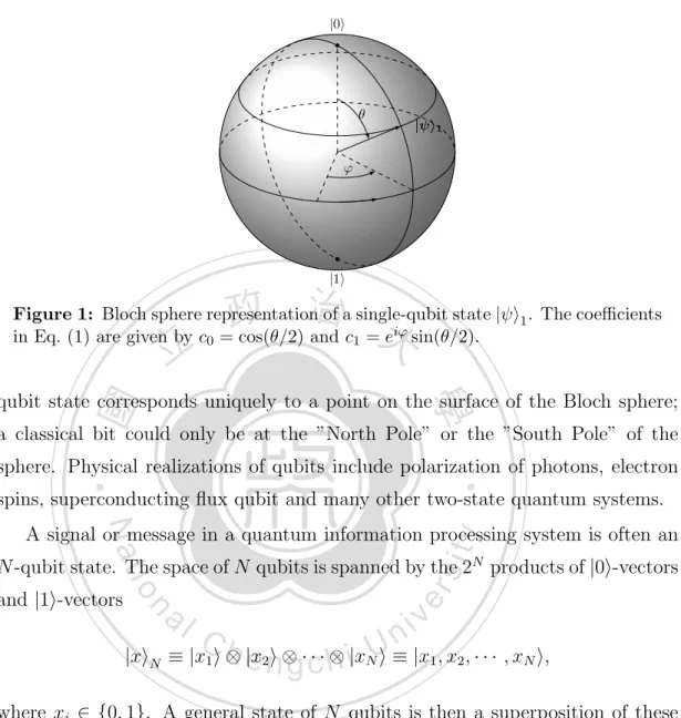
(12) Introduction. |0i. ✓. | i1. '. |1i. 政治大. Figure 1: Bloch sphere representation of a single-qubit state | i1 . The coefficients in Eq. (1) are given by c0 = cos(✓/2) and c1 = ei' sin(✓/2).. 立立. •‧ 國. ㈻㊫學. qubit state corresponds uniquely to a point on the surface of the Bloch sphere; a classical bit could only be at the ”North Pole” or the ”South Pole” of the. •‧. sphere. Physical realizations of qubits include polarization of photons, electron spins, superconducting flux qubit and many other two-state quantum systems.. Nat. sit. y. A signal or message in a quantum information processing system is often an. al. iv n C |xiN ⌘ |x1 i h ⌦e |x2n i ⌦ · · ·h g c ⌦ i|xNUi ⌘ |x1, x2, · · · , xN i, n. and |1i-vectors. er. io. N -qubit state. The space of N qubits is spanned by the 2N products of |0i-vectors. where xi 2 {0, 1}. A general state of N qubits is then a superposition of these 2N product states. | iN =. X. 0x<2N. cx |xiN. and cannot, in general, be expressed as a product of a set of one-qubit states. Such non-product states of many qubits are called entangled states. A quantum algorithm consists of a sequence of unitary transformations (gates) applied on N qubits. Any unitary transformation U satisfies the condition U U † = U † U = I,. 2.

(13) where I is the identity operator; that is a unitary transformation preserves the magnitudes of all vectors, h | i = hU |U i = h |U † U | i. In order to provide an output at the end of a computation, we need a measurement gate, which can be thought of as a projection on the basis states. A particular basis state, |xi, will be measured with a probability given by the squared mag-. nitude of the amplitude of the state, |cx |2 , in the expansion of the state that is being measured. In contrast to unitary gates, which have a unique output state. 政治大 only statistically determined by the state of the input qubits. 立立 Many algorithms have been designed based on qubits and quantum gates, such. for each input state, the state of the qubits resulting from a measurement gate is. •‧ 國. ㈻㊫學. as Shor’s algorithm [2] for integer factorization, and Grover’s search algorithm [3]. Developments in quantum algorithm design after Shor’s and Grover’s algorithms. •‧. have been mainly focused on generalizations of these two types of algorithms.. y. sit. on classical computers.. Nat. Recently, two alternative trends have entered the field, quantum walks and adiabatic quantum algorithms – this thesis is concerned with these two algorithms. n. al. er. io. This thesis is organized into two parts. In Part I, we investigate the quantum. i Un. v. walks, both the discrete-time version and the the continuous-time version; In Part II, we focus on optimization by quantum adiabatic algorithms; in particular, we. Ch. engchi. implement quantum Monte Carlo annealing to find ground states of Ising spin glasses.. 3.

(14) Introduction. 立立. 政治大. •‧. •‧ 國. ㈻㊫學. n. er. io. sit. y. Nat. al. Ch. engchi. 4. i Un. v.

(15) 政治大立立Part I. •‧ 國. ㈻㊫學. Quantum Random Walks •‧. n. er. io. sit. y. Nat. al. Ch. engchi. 5. i Un. v.


(17) 1 Part I – Introduction 政治大立立 of probability distribution of particles or Random walks describe the evolution •‧ 國. ㈻㊫學. states in a structured space. Many natural phenomena, such as the trajectory of a molecule traveling in a gas/liquid, the foraging behavior of insects, evolution of stock market prices, and energy transfer process in photosynthesis, can be. •‧. modeled in terms of random walks. There are countless applications based on. y. sit. of science.. Nat. random walks in physics, biology, chemistry, economics, and many other branches. er. io. Mathematical models of random walks have been developed into many useful computational algorithms, such as Monte Carlo methods, algorithms for decision. n. al. Ch. i Un. v. problems, search algorithms and algorithms for optimization problems. Inspired. engchi. by the versatility of random walks, quantum walks have been proposed and designed for quantum algorithms, which could be run directly and efficiently on quantum computers [1]. Quantum walks described by quantum mechanical wave functions have very di↵erent properties from classical random walks; for example, they do not in general converge toward a stationary distribution and potentially spread much faster. Quantum walks have been demonstrated with trapped ions [4], optically trapped atoms [5], correlated photons [6]. It is noteworthy that quantum walks have been applied to studying energy transport in plants, providing theoretical models of photosynthesis [7]. In general there are two di↵erent types of quantum walks, the discrete-time quantum walk and the continuous-time quantum walk, which are both considered. 7.

(18) Part I – Introduction. in the first part of this thesis. Comparisons of results for quantum walks and classical random walks will be made in many examples, ranging from random walks on graphs to walks in disordered media.. 立立. 政治大. •‧. •‧ 國. ㈻㊫學. n. er. io. sit. y. Nat. al. Ch. engchi. 8. i Un. v.

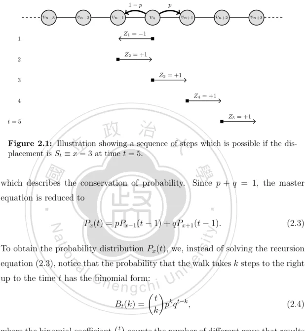
(19) 2. The simple random walk on a line. ㈻㊫學. 2.1.1. •‧ 國. Classical Random Walks 政治大立立 2.1 The one-dimensional random walks •‧. We first consider the simplest case, a Bernoulli walk on a one-dimensional (1D). Nat. lattice. We define the lattice sites (vertices) {vn : n 2 Z} on the integer number. sit. y. line, Z. A random walk on the line is a process that begins at some vertex, say. er. io. vn , and at each time step t, assumed to be discrete with t = 0, 1, 2, · · · , moves either to the neighboring site vn+1 with a probability denoted by wn,n+1 or to. al. iv n C h e nentirely the next state depends the current state and not i U g c hon n. vn. 1. with probability wn,n 1 . This process can be considered as a memoryless. Markov chain, i.e. on previous states.. We define Zj as the direction of movement at time step t = j; The sequence Z1 , Z2 , · · · , Zj , · · · is thus a set of independent random variables, taking either 1 or. 1. The sum. St = Z 1 + Z2 + · · · + Zt gives the net displacement of the walk at time t wn,n+1 = p and wn,n. 1. = q = 1. (2.1) 1 (i.e. after t steps). Let. p for all vertex vn . Denote the value of the. displacement St by x (2 Z). The probability Px (t) of the displacement at time t evolves deterministically and obeys the so-called master equation ⇥ ⇤ ⇥ ⇤ Px (t) = Px (t 1) + pPx 1 (t 1) + qPx+1 (t 1) pPx (t 1) + qPx (t 1) , (2.2). 9.

(20) Classical Random Walks. 1 vn. vn. 3. vn. 2. p. p. Z1 =. 1. vn+1. vn. 1. vn+2. vn+3. 1. Z2 = +1. 2. Z3 = +1. 3. Z4 = +1. 4. Z5 = +1. 政治大 Figure 2.1: Illustration showing a sequence of steps which is possible if the displacement is S ⌘ x立立 = 3 at time t = 5.. t=5. t. •‧ 國. ㈻㊫學. which describes the conservation of probability. Since p + q = 1, the master. •‧. equation is reduced to. 1).. (2.3). y. 1) + qPx+1 (t. sit. Nat. Px (t) = pPx 1 (t. al. er. io. To obtain the probability distribution Px (t), we, instead of solving the recursion. v. n. equation (2.3), notice that the probability that the walk takes k steps to the right. Ch. up to the time t has the binomial form:. e n g c ✓h i◆ Bt (k) =. where the binomial coefficient. t k. i Un. t k t k p q , k. (2.4). counts the number of di↵erent ways that results. in k steps to the right among t total steps, while the factor pk q t probability for a single such walk. From x = 2k. k. gives the. t, we can conclude that t and. x must have the same parity, and the probability distribution is given by Px (t) =. (. Bt ((x + t)/2) , if x and t are both even or both odd, 0, otherwise.. Hence one obtains the mean displacement hxi =. 10. P. x. xPx and the variance. (2.5) 2 x. ⌘.

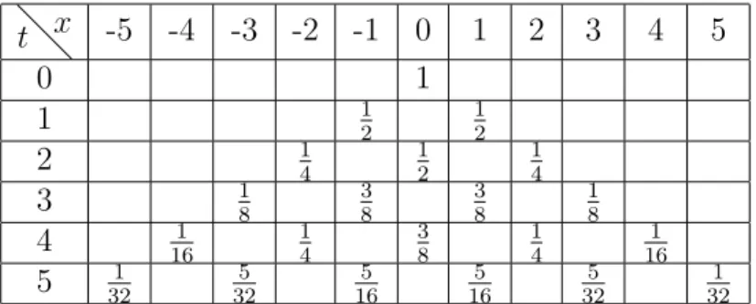
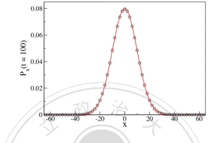
(21) 2.1 The one-dimensional random walks. t x 0 1 2 3 4 5. -5. 1 32. -4. -3. 1 8. 1 16. 5 32. -2. 1 4 1 4. -1 1 2 3 8 5 16. 0 1 1 2 3 8. 1. 2. 1 2. 1 4. 3 8 5 16. 1 4. 3. 4. 1 8. 5. 1 16. 5 32. 1 32. Table 2.1: Time evolution of the probability of the displacement up to t = 5 for a symmetric random walk on the line.. hx2 i. hxi2 :. 政治大 q), = 4tpq. 2 x. hxi = t(p. 立立. (2.6). •‧ 國. ㈻㊫學. If t ! 1, and p is far from zero or one, the binomial distribution in Eq. (2.5). converges towards a Gaussian distribution 1 e 2⇡tpq. [x t(p q)]2 /8tpq. .. •‧. Px (t) ! p. (2.7). y. Nat. This convergence, as a consequence of the central limit theorem, arises indeed. sit. independent of the form of the single-step distribution as long as the single steps. al. n. finite.. er. io. are uncorrelated and the first two moments of the single-step distribution are. Ch. i Un. v. Consider for example the case of the symmetric random walk with p = q =. engchi. 1/2. The probability Px (t) of being at a position x away from the starting point after up to t = 5 steps is given in Table 2.1. Fig. 2.2 shows a comparison between the probability distribution and its Gaussian approximation.. 2.1.2. A one-dimensional random walk in a random medium. In many practical cases the medium where the random walk is performed is irregular due to impurities, defects or intrinsic randomness. If temporal changes in the medium occur on a much larger scale than the time scale associated with the walk, we can treat the randomness in the medium as time independent. To model a random walk in an environment with static disorder (called ”quenched disorder”), we assume that the transition probabilities {wm,n } are inhomogeneous. 11.

(22) Classical Random Walks. 0.08. Px(t = 100). 0.06. 0.04. 0.02. 0. -60. 立立. 政治大 x. -40. -20. 0. 20. 40. 60. •‧. •‧ 國. ㈻㊫學. Figure 2.2: Probability distribution of the displacement x for the symmetric random walk with p = q = 1/2 at time t = 100. The data in open circles are generated using the recursion relation (2.3). Only data points with even values of x are shown; the probability Px (t) for odd values of x is zero since x and t = 100 have opposite parity. The red solid line is the Gaussian approximation given in Eq. (2.7).. sit. y. Nat. er. io. and site dependent; the environment is then determined by the sequence of random variables {wm,n }. For the nearest-neighbor one-dimensional walk that we. n. al. Ch. i Un. v. consider here, we will parameterize the transition probabilities as. engchi. wn,n+1 = pn , wn,n. 1. =1. (2.8). pn ,. where the probabilities pn > 0 are independent and identically distributed random variables. We note that in general the transition probabilities are not symmetric, wn,n±1 6= wn±1,n . Denote by Pn (t) the probability for the walk to be at site vn at time t. The master equation for Pn (t) is a linear recursion relation Pn (t) = pn 1 Pn 1 (t. 1) + (1. pn+1 )Pn+1 (t. 1).. (2.9). Concerning the mean value of some quantity, Q, in the presence of quenched. 12.

(23) 2.1 The one-dimensional random walks. wn,n. vn. 立立 v. 2. n. wn+1,n. 政治大 w w 1. n 1,n. n,n+1. vn+1. vn. 1. vn+2. •‧. •‧ 國. ㈻㊫學. Figure 2.3: The motion of the random walk in a random environment resembles the motion of a particle in a random potential.. disorder, we should distinguish two di↵erent types of averages: (i) the configura-. y. Nat. tion average, denoted by hQi, is the average over di↵erent ”histories” in a fixed. sit. environment (i.e. for a fixed set of {pn }); (ii) the disorder average, denoted by. er. io. [Q]av , is obtained by averaging over many independent realizations of the random. al. n. iv n C What makes the random walk inha e random environment n g c h i U particularly inter-. environment according to a given distribution.. esting is anomalous dynamics in which the time dependence of the mean square displacement deviates from the linear form. 2 x. / t as given in Eq. (2.6). As an ex-. ample, let us consider the so-called Sinai’s walk[8], which satisfies the condition: . ✓. pn log 1 pn. ◆. = 0;. (2.10). av. under this condition the random walk is recurrent in that it visits the starting point infinitely often.1 In his seminal work [8], Sinai showed rigorously that the mean square displacement (averaged over the histories and all environments) for 1. In the absence of disorder, the symmetric walk with p = q = 1/2 in 1D is also recurrent. If a random walk may return to the origin only finitely many times, the walk is called transient.. 13.

(24) Classical Random Walks. the case of zero drift has the form [hx2 (t)i]av / log4 (t),. (2.11). indicating extremely strong slowdown of the motion in a random medium as compared with the di↵usive behavior of the ordinary random walk in a homogeneous medium. Fig. 2.4 shows the time evolution of the disorder-averaged quantity [hx2 (t)i]av for the Sinai model with random transition probabilities {pn } which are uniformly distributed in the interval (0, 1).. 政治大. 立立 3. 2. 10. •‧. 2. av. ㈻㊫學. •‧ 國 [ <x > ]. 10. 1. Nat. y. 10. 0. 1. n. al. Ch. i Un. log(t). engchi. er. io. sit. 10. 10. v. Figure 2.4: Time evolution of the mean square displacement [hx2 i]av (solid line) in a log-log plot. The data obtained by using the master equation (2.9) are averaged over 1000 samples of the random environment with {pn } being uniform random variables on (0, 1). In the large t regime, [hx2 i]av grows as log4 (t), as indicated by the red dashed line; in early times when disorder is irrelevant, the motion is normal di↵usive and [hx2 i]av grows linearly with t, as shown by the green dashed line.. The time-length scaling (2.11) in the long-time limit can be explained via a simple argument [9]. One introduces a potential for the model: Un. U0 =. n 1 X. log(pi ). log(1. pi ) ,. (2.12). i=1. where the subscript n denotes site vn . Since the random potential itself is a sum. 14.

(25) 2.2 Random walks on graphs. of independent random variables, it follows that Un ⇠ for n. p. n,. (2.13). 1. From the Arrhenius Law [10], we obtain the time that the walker. needs to escape from the potential well grows exponentially with depth of well t ⇠ e Un ⇠ e. p. n. .. (2.14). Thus the di↵usion follows a logarithmic law as given in Eq. (2.11). We note that. 政治大 t ! 1. Instead, in early times 立立the disorder e↵ect is not significant; the motion. the argument given above is valid only insofar as n in Eq. (2.12) is large and thus. •‧ 國. ㈻㊫學. in this regime is normal di↵usive and [hx2 i]av grows linearly with t (as indicated by the green dashed line in Fig. 2.4).. •‧. Random walks on graphs. sit. y. Nat. 2.2. er. io. So far we have considered one-dimensional random walks. The generalization to random walks in higher dimensions is straightforward. Here we also restrict. n. al. Ch. ourselves to the case of discrete spaces, i.e. graphs.. engchi. i Un. v. We consider a connected graph G = (V, E) consisting of a set of vertices (or nodes) V = {vn : n 2 Z} connected by a set of edges E = {(vm , vn )}. The. number of the vertices |V | may be finite or infinite. We assume that the graph is undirected in the sense that the relations between pairs of vertices are symmetric, and each edge has no directional character. Each edge (vm , vn ) connecting a pair of vertices has a weight wm,n > 0 denoting the probability to reach vn from vm in one time step t. These transition probabilities govern a random walk along the vertices of the graph G. In fact, the one-dimensional random walk on the integer line that we considered in Sec. 2.1.1 is a simple example of random walks on a graph with |V | = 1. For a given graph and a set of the transition probabilities {wm,n }, one can write down the master equation as a gain-loss equation for the. 15.

(26) Classical Random Walks. probability Pn (t) of finding the walker at vertex vn at time t: Pn (t + 1) = Pn (t) +. X. X. wm,n Pm (t). m6=n. |. {z. m6=n. }. gain. wn,m Pn (t) .. |. {z. loss. (2.15). }. The second term of the right-hand side is the gain of vertex vn due to transitions from other vertices vm , and the third term is the loss due to transitions from vn into other vertices. Eq. (2.15) can be written as a linear map 1) = W P (t) , 政P (t + 治大 ~. 立立. ~. (2.16). where P~ (t) is a probability vector given by P~ (t) = (· · · , Pn 1 (t), Pn (t), Pn+1 (t), · · · )T ,. •‧ 國. ㈻㊫學. and W is the so-called stochastic matrix. The entry Wmn is just the transition. probability wn,m ; for example, for the random walk on a line with equal probability of moving to the left and to the right, the stochastic matrix is given by the. n. Ch. 1 2. y. 0. 1 2. 1 2. 0. engchi. 1 2. C C C C C. C C A. sit. io. al. B B B B W =B B B @. 1. ... 1 2. er. Nat. 0. •‧. band diagonal matrix. iv n U .. 0. 1 2. .. (2.17). An initial probability distribution P~ (0) will become P~ (t) = W t P~ (0) after t steps of the walk. If the underlying graph G is connected and non-bipartite, then the distribution P~ (t) of the random walk converges to a stationary distribution P~ ⇤ . For the stationary distribution P~ ⇤ , we have W P~ ⇤ = P~ ⇤ . It is often more convenient to consider random walks indexed by continuous time t 2 R+ . In this case, the master equation becomes a linear partial di↵erential equation:. X @ Pn (t) = wm,n Pm (t) @t m6=n. wn,m Pn (t) ,. (2.18). where the coefficients wm,n are transition rates, i.e. transition probabilities per. 16.

(27) 2.2 Random walks on graphs. v1. v4. v5. v2. v3. Figure 2.5: An undirected graph with five vertices.. time unit. t ! 0. Thus wm,n may be larger than 1.. 政治大 written as a set of coupled linear 立立 di↵erential equations, or in a compact matrix The master equation (2.18) for each vertex in the graph with |V | = N can be. form. •‧ 國. ㈻㊫學. @ ~ P (t) = @t. M P~ (t). (2.19). •‧. with a transition rate matrix M (or known as the generator operator). The. m,n. X. wn,k ,. k6=n. n. al. X. Ch. engchi. Mmn  0, for m 6= n,. m. i Un. Mmn = 0, 8 n.. (2.20). er. io and satisfy the conditions:. wn,m +. sit. Nat. Mmn =. y. elements of the N ⇥ N transition rate matrix are given by. v. (2.21). If the transition rate on each edge in G is a constant , the transition rate matrix M reads Mmn =. 8 > > > <. dn ,. v n = vm (vm , vn ) 2 E. , > > > :0,. (2.22). otherwise.. where dn is the degree (or valence) of the vertex vn , i.e. the number of edges at vn . For example, a simple random walk on the graph defined in Fig. (2.5) with a constant transition rate wm,n =. on all edges (vm , vn ) 2 E, the transition rate. 17.

(28) Classical Random Walks. matrix M is given by 0 B B B B B B @. M=. 2 1 0 1 1. 1 2 1 0 1. 0 1 2 1 1. 1 1 C 1C C 1C C. C 1A 4. 1 0 1 2 1. (2.23). The solution of the master equation (2.19) with given initial probability distribution P~ (0) is formally given by. 立立. 政治大 P~ (t) = exp( M t)P~ (0).. (2.24). •‧ 國. ㈻㊫學. In order to determine P~ (t) for the case of finite N explicitly, one often needs to k. and the eigenvectors ~uk of M , and then construct. •‧. the solution as a superposition of ~uk ↵k e. kt. k. ~uk ,. (2.25). er. io. X. sit. Nat. P~ (t) =. y. first obtain the eigenvalues. al. iv n C for solving Eq. (2.19), however, be used as a general method, because it h e ncannot hi U c g requires that M is diagonalizable. n. where the coefficients ↵k are determined by the initial condition. This method. Now we consider the continuous time version of the symmetric random walk on the integer line Z with |V | = 1. Without loss of generality, we assume wn,n±1 = 1. The master equation for Pn (t) is @Pn = Pn+1 + Pn @t. 1. 2Pn .. (2.26). This equation can be solved via the discrete Fourier transform P˜k (t) =. 1 X. n= 1. 18. Pn (t) eikn .. (2.27).

(29) 2.3 Mapping between random walks and quantum spin systems. Fourier transforming both sides of Eq. (2.26), we obtain @ P˜k (t) ⇥ ik = (e + e @t. ik. ⇤ 2 P˜k (t).. ). We suppose that the initial condition is Pn (0) =. n,0 .. (2.28) Since P˜k (0) = 1, the. solution to Eq. (2.28) is P˜k (t) = e2(cos k. 1)t. .. (2.29). By comparing Eq. (2.29) with the Jacobi-Anger expansion [11] in terms of the. 治政大 X. n-th Bessel function of first kind, Jn (z),. 立立=. 1. in Jn (z)eink ,. n= 1. we obtain the solution. n. 2t. ,. (2.31). •‧. io. Pn (t) ! p. n. al. Ch. 1 e 4⇡t. n2 /4t. ,. sit. y. Nat. Jn (it) is the modified Bessel function of order n. In the long p time limit, this expression is approximately a Gaussian function of width 2t. er. where In (t) = (i). Pn (t) = In (2t) e. (2.30). ㈻㊫學. •‧ 國. e. iz cos k. i Un. (2.32). v. in agreement with the long-time behavior of the discrete time version.. 2.3. engchi. Exact mapping between classical random walks and equilibrium quantum spin systems. Great progress has been achieved in solving certain stochastic processes by the realization of the connection between the formalism for those problems and that for quantum many-body systems. More specifically, the master equation (2.19) of a stochastic system may be reformulated as a Schrödinger equation 1@ |P (t)i = i @t. 19. H|P (t)i. (2.33).

(30) Classical Random Walks. in terms of a Hamiltonian H of a quantum spin system. This has allowed the stochastic models to be solved by exact analytic techniques of equilibrium statistical mechanics. Or, conversely, the corresponding quantum problems can be solved by techniques for stochastic models. In this section, we will show an example of this type of approach [9, 12]: the mapping of the one-dimensional random walk to the quantum Ising chain described by the Hamiltonian X. H=. z n. Jn. X. z n+1. x n. n. ,. (2.34). 政治大 in terms of the Pauli spin operators { } located on the sites (vertices) {v } of 立立 a one-dimensional lattice. Here {J } are the nearest-neighbor ferromagnetic coun. n. x,z n. n. n. •‧ 國. n}. represent on-site transverse fields. In the quantum computing. ㈻㊫學. plings, and {. terminology, we can say that the system is a set of interacting ”qubits”. Without. •‧. the transverse fields, the spin Hamiltonian is reduced to a classical Ising Hamiltonian since each spin is in one of the eigenstates {| "i, | #i} of. z. ; in this case,. al. O. |"in. |+i =. and. O. er. io. |*i =. sit. y. Nat. the Hamiltonian has two possible ferromagnetic ground states |#in ,. (2.35). n. iv n C with all spins parallel. Thehnon-commutingU e n g c h i transverse field term induces quantum fluctuations changing the system’s ground state to a non-trivial quantum n. n. superposition of all possible spin configurations. One of the standard analytic techniques for solving the quantum Ising chain is free-fermion diagonalization [13]. Using the Jordan-Wigner transformation [14] and a subsequent canonical transformation [13], we can map the interacting quantum Ising chain into spinless free fermions Hfermion =. X. "q. q. ✓. ⌘q† ⌘q. 1 2. ◆. .. (2.36). where ⌘q† and ⌘q are fermion creation and annihilation operators, respectively. The fermionic excitation energies "q for a chain of length N (. 20. 1) with free boundary.

(31) 2.3 Mapping between random walks and quantum spin systems. condition (i.e. JL = 0) can be obtained by solving the eigenvalue equation T | q i = "2q | q i. (2.37). for the 2L ⇥ 2L symmetric matrix: 0. B B B B B T =B B B B @. 0 1. 1. 1. 0 J1. 立立. J1 0 .. .. 2. ... ... .. .. C C C C C C. C C C LA 0. (2.38). 政J 治0 大 L 1. L. •‧ 國. ㈻㊫學. Here we are particularly interested in the general case, in which the couplings and fields are random variables.. •‧. Consider now a one-dimensional random walk in a random environment, characterized by transition rates wn,n±1 for a move from site vn to site vn,n±1 . The walk. y. Nat. sit. is confined in a finite segment between site v1 and site vL ; the one-dimensional. al. er. io. lattice has two adsorbing sites located at v0 and vL+1 so that w0,1 = 0 and. v. n. wL+1,L = 0. The time evolution of the probability Pn (t) for the walker to be on. Ch. i Un. site vn at time t is governed by a master equation (cf. (2.19)) with a transition. engchi. rate matrix, M , whose elements take the form Mn,n±1 =. wn±1,n. and. Mn,n = wn,n. 1. + wn,n+1 .. (2.39). Solving the master equation amounts to solving the eigenvalue problem for the transition rate matrix M~uq =. uq q~. ,. (2.40). with ~uq = (uq (1), uq (2), · · · , uq (L))T . This eigenvalue equation can be rewritten as. X m. fm,n u M eq (n) =. 21. eq (n) , qu. (2.41).

(32) Classical Random Walks. in terms of the new variables n Y wm,m+1 u e(n) = u(n) w m=1 m+1,m. !. 1/2. .. (2.42). f has become symmetric Through this transformation the transition rate matrix M and is given by 0. 政治大. •‧ 國. 立立. 1. C C C C C C. C C p C wL,L+1 A 0. .... p. 0 wL,L+1. ㈻㊫學. p 0 w1,2 Bp p B w1,2 0 w2,1 B p p B w2,1 0 w2,3 B f=B M . . .. .. B B p B wL,L 1 @. (2.43). Comparing Eqs. (2.38), (2.37), (2.43) and (2.41), we notice that the exact map-. •‧. ping between the quantum Ising chain and the 1D random walk with the following. n. n. al. Ch. , ,. p. wn+1,n. p. wn,n+1. er. io. Jn. q .n U engchi. "2q. ,. sit. y. Nat. correspondences:. (2.44). iv. Aside from the results for the 1D random walks we discussed in the previous sections, one can extract many other exact results from this mapping, for example, the probability for a single walker not to return to the starting point up to t. This survival probability, calculated with adsorbing boundary conditions w0,1 = wL+1,L = 0, converges to a finite value denoted by Ps (L) in the long time limit t ! 1, which is given by an exact expression [12, 15] Ps (L) =. L Y n X wm,m 1 1+ w n=1 m=1 m,m+1. !. 1. .. (2.45). In the quantum Ising chain mapping, the expression (2.45) corresponds to an. 22.

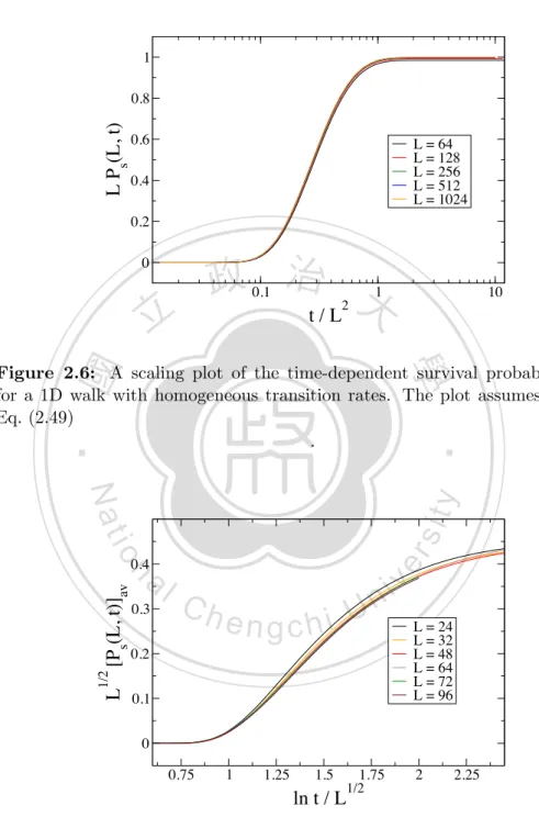
(33) 2.3 Mapping between random walks and quantum spin systems. exact formula for the surface magnetization of the chain: (ms (L))2. ,. Ps (L) .. (2.46). For a homogeneous medium with wn,n+1 = wn+1,n = const, we obtain Ps (L) / (L + 1). 1. .. (2.47). For a random medium without drift, an exact result has been found for the disorder-average survival probability [9, 12]. 政 with治✓ = 1 .大 2. [Ps (L)]av / L ✓ ,. 立立. (2.48). •‧ 國. ㈻㊫學. Combining the size-dependent survival probabilities (Eqs. (2.47) and (2.48)) with p the known relations between the characteristic time and length, L ⇠ t for a homogeneous random walk, and L ⇠ ln2 (t) for a disordered random walk, one. •‧. can further deduce the finite-size scaling form for the time-dependent survival. al. n. and in a random environment [12]. sit. io. Ps (L, t) = LPes (t/L2 ) ,. (2.49). er. Nat. y. probability in a homogeneous medium. ni C h 1/2 U i ). h 1/2 [Ps (L, t)]av = L e n Pesg (lnct/L. v. (2.50). We have verified these results by recursive implementations of the master equations for discrete random walks; the finite-size scaling is depicted in Fig. (2.6) and Fig. (2.7).. 23.

(34) Classical Random Walks. 1. L Ps(L, t). 0.8 0.6. L = 64 L = 128 L = 256 L = 512 L = 1024. 0.4 0.2. 政治大 t/L. 0. 0.1. 立立. 1. 2. 10. •‧ 國. ㈻㊫學. Figure 2.6: A scaling plot of the time-dependent survival probability Ps (L, t) for a 1D walk with homogeneous transition rates. The plot assumes the form in Eq. (2.49). •‧. .. er. io. sit. y. Nat 0.4. 0.3. Ch. engchi. i Un. 0.2. L. 1/2. [Ps(L, t)]av. n. al. 0.1. v. L = 24 L = 32 L = 48 L = 64 L = 72 L = 96. 0 0.75. 1. 1.25. 1.5. ln t / L. 1.75. 1/2. 2. 2.25. Figure 2.7: A scaling plot of the disorder-averaged survival probability Ps (L, t) for a 1D walk with asymmetric random transition rates drawn from a uniform distribution. The data are averaged over 105 disorder realizations. The plot assumes the scaling form in Eq. (2.50). .. 24.

(35) 3 Discrete-Time Quantum Walks 政治大立立 Quantum walks were initially introduced in both continuous [17] and discrete [18] •‧ 國. ㈻㊫學. time, in analogy with their classical counterparts. The major di↵erence between these two types of quantum walks lies in the definition of the evolution operator.. •‧. A quantum computer would work with discrete registers; discretizing the position space of the quantum walk will allow us to map it to algorithms on such a machine.. y. Nat. Therefore, we will only focus on quantum walks discrete in space, i.e. quantum. al. er. io. walks.. sit. walks on graphs. In this chapter we will first consider discrete-time quantum. v. n. In the simplest discrete-time classical random walk on a graph G = (V, E),. Ch. i Un. at each time step the walker simply moves from any given vertex to each of its. engchi. neighbors with equal probability. Thus the walk is governed by the |V | ⇥ |V | matrix W with elements. Wmn =. 8 <1/d. (vm , vn ) 2 E. n. :0. (3.1). otherwise,. where dn is the degree of the vertex vn . After one step of the walk, an initial probability distribution P~ over the vertices evolves to P~ 0 = W P~ . The quantum version of the discrete-time random walk can broadly be defined as the repeated application of a unitary evolution operator at each time step, without performing intermediate measurements. To define a quantum walk, we need to specify a unitary operator U with the property that an input state |ni,. 25.

(36) Discrete-Time Quantum Walks. corresponding to the vertex vn 2 V , evolves to a superposition of the neighbors of vn . It has turned out that to define such a unitary operator one needs to. enlarge the Hilbert space by adding an ancillary system storing the direction in which the walk is moving [19]. The Hilbert space of discrete-time quantum walks is often the tensor product of the position space Hp and a so-called ”coin space” Hc . The position space is a |V |-dimensional Hilbert space spanned by. orthonormal basis vectors, {|ni : n = 1, · · · , |V |}, corresponding to the vertices of the graph. Associated with each vertex vn is also a set of ”coin states” {|cm i :. 政治大. m = 1, · · · , dn }, where dn is the degree of the vertex vn ; these coin states represent. the outgoing edges of each vertex and span the coin space. Basis vectors of the. 立立. Hilbert space of the walk H = Hp ⌦ Hc are then product states of the form. •‧ 國. ㈻㊫學. |ni ⌦ |cm i ⌘ |n, cm i. This type of discrete-time quantum walk is sometimes referred to as the coined quantum random walk.. X m,n. ↵ ↵m,n (t) n, cm ,. y. Nat. | (t)i =. (3.2). sit. as. •‧. Being an element in H, a general state of the quantum walker can be written. er. io. where ↵m,n (t) (2 C) is the probability amplitude associated with the walker being. al. n. iv n C application of a given unitary h etime h i Uoperator U on | (t)i. The unitary n gevolution c time evolution of a discrete-time quantum walk is generally defined as [19]. at vertex vn with the coin state |cm i at time t. One step of the walk is the. U = S · Ip ⌦ C ,. (3.3). where S is the shift operator, C is the so-called coin operator, and Ip denotes the identical operator on the position space. For a vertex vn of degree dn the coin operator C defined on Hc can be represented by a dn ⇥dn matrix. Various choices of the coin operator are possible as long as the operator is unitary. For a given. graph, one can define a rich family of walks with di↵erent behavior by changing C. After the application of the operator C, the shift operator S applies a conditional translation to the position state according to the coin state. A quantum walk. 26.

(37) with the initial state | (0)i after t steps is then described by the equation | (t)i = U t | (0)i,. (3.4). resulting in propagation of probability amplitudes across the graph. For a discrete-time quantum walk on a line, we need to specify a 2 ⇥ 2 coin. matrix since the coin space Hc for this case must be spanned by two basis states, denoted by |. i and | !i, corresponding to two possible outgoing edges on a. vertex. This coin operator may be any U(2) operator (i.e. 2 ⇥ 2 unitary matrices) parameterized by. 0. 1 sin ✓ 政 e治 A大 .. ei cos ✓. C=@. 立立e. i⌘. i⌘. sin ✓. e. i. (3.5). cos ✓. •‧ 國. ㈻㊫學. After ”tossing” the coin with the coin operator, a conditional translation is made by the shift operator in the way that the walker moves one step to the left if the i, or to the right if the accompanying coin state. •‧. accompanying coin state is |. ih. io. al. | +. ✓X n. ◆. |n + 1ihn| ⌦ | !ih! | .. sit. 1ihn| ⌦ |. ◆. (3.6). er. n. |n. Nat. S=. ✓X. y. is | !i. The shift operator for this operation is expressed mathematically as. v. n. One example for the coin operator is the Hadamard coin given by. Ch. !. 1 g 1c h i en ,. 1 (2) CH = p 2. 1. 1. i Un. (3.7). corresponding to the operator in Eq. (3.5) with ✓ = ⇡/4, ⌘ = 0 and. = ⇡/2.. Assume now that the initial state is | (0)i = |ni ⌦ | !i ⌘ |n, !i. One step of the quantum walk governed by the Hadamard coin is thus |ni ⌦ | !i. ↵ ↵ 1 1 ! p !, n + p ,n 2 2 ↵ 1 1 ! p !, n + 1 + p ,n 2 2. CH. S. ↵. (3.8). 1 .. The position state resulted from the action of the unitary operator U is an equal superposition of the left vertex and the right vertex, which is fundamentally dif-. 27.

(38) Discrete-Time Quantum Walks. ferent from an equal mixture of these two components. Indeed, the interference between di↵erent positions in the graph will cause a behavior radically di↵erent from that of a classical random walk. If we, however, perform a measurement at some point in order to know the outcome of the walk, quantum interference will be destroyed. With a measurement at each step of the walk, we will revert to the classical ransom walk. To illustrate the feature of the quantum walk, we perform the walk starting with the initial state |n = 0i ⌦ | !i without intermediate measurements up to t steps. A measurement on the position is performed at time t by using the projection operator. 立立. 政 ⇤治 = |nihn|大 ;. (3.9). n. •‧ 國. ㈻㊫學. the probability that the walker is in the vertex state |ni at time t is given by Pn (t) = h (t)|⇤n | (t)i .. (3.10). •‧. The probability distribution over the graph after t = 100 steps is shown in Fig. 3.1.. y. Nat. The distribution looks markedly di↵erent from the analogous classical distribu-. sit. tions. Peculiar features include the asymmetry structure and the relative uni-. al. er. io. formity of the central portion of the distribution, in contrast to the classical. v. n. Gaussian distribution. The asymmetry of the quantum distribution arises from. Ch. i Un. the fact that the Hadamard coin operator does not treat | !i and |. e gchi states in the same way (cf. Tab.n3.1). t n 0 1 2 3 4 5. -5. 1 32. -4. 1 16. -3. 1 8 5 32. -2. 1 4 1 8. -1 1 2 1 8 1 8. 0 1 1 2 1 8. 1 1 2 5 8 1 8. 2. 1 4 5 8. 3. 1 8 17 32. 4. 1 16. i coin. 5. 1 32. Table 3.1: The probability of being found at position |ni after t steps of the quantum random walk on the line with a Hadamard coin and the initial state | (0)i = |0, !i. Note that this distribution starts to show a drift to the right from t = 3 on.. 28.

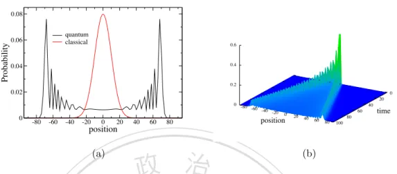
(39) Probability. 0.15. 0.1. 0.05. 0. -80. -60. -40. 立立. -20. 0. 20. 40. 60. 80. 政治大 position. •‧ 國. ㈻㊫學. Figure 3.1: Position probability distribution after 100 time steps for a quantum walk on a line using a Hadamard coin defined in Eq. (3.7), and the initial state |0, !i. Only even positions are shown, since odd positions have probability zero.. n. al. Alternatively, we can use an unbiased coin, like. Ch. (2) Csymm. e n1g ci !h i. 1 =p 2. i 1. sit. ↵. .. i Un. ,. (3.11). er. io. ↵ 1 | (0)i = p 0, ! + i 0, 2. y. i, for example,. Nat. superposition of | !i and |. •‧. To obtain a symmetric position distribution, we can use an initial state as a. v. (3.12). to generate a symmetric distribution. The position probability distribution at t = 100 using the Hadamard coin operator with the initial state (3.11) (or the unbiased coin Csymm with the initial state |0, !i) is depicted in Fig. 3.2. It is. apparent that the distribution is almost uniform over the interval [ t/a, t/a] (it p can be shown analytically [20, 21] that a = 2), and strongly peaked at the edges 2. at ±t/a. Thus, the variance. is approximately given by t/a. 2. aX 2 = hn i ⇡ n / t2 . t 1 2. 29. (3.13).

(40) Discrete-Time Quantum Walks. Probability. 0.08 quantum classical. 0.06. 0.04. 0.02. 0. -80. -60. -40. -20. 0. 20. position. 40. 60. 80. (a). (b). 治政 Figure 3.2: (a) Position probability distribution 大 (black line) after 100 time steps for a quantum walk立立 on a line using the Hadamard coin operator, and the symmetric initial state given in Eq. (3.11). Only even positions are shown, since odd positions •‧. •‧ 國. ㈻㊫學. have probability zero. The red line corresponds to the distribution for a classical random walk; (b) evolution of the probability distribution from time t = 1 up to t = 100.. sit. y. Nat. This linear time dependence of the variance implies that the quantum walk prop-. al. n. / t).. io. 2. er. agates quadratically faster than the classical symmetric random walk (which has. Ch. i Un. v. A discrete-time quantum random walk can be defined for arbitrary undirected. engchi. graphs by using di↵erent position and coin spaces [19]. We consider here a twodimensional (2D) lattice. Again, the position space is spanned by all vertices of the graph. We often use a pair notation |nx , ny i to identify the x- and ycomponents of vertex |ni. Each vertex in a 2D lattice has four edges connected to it, so the coin operator is now a four-dimensional unitary operator. We label the four directions |. i, | !i corresponding to the two directions on the x-axis. and | "i, | #i for two directions on the y-axis. A common choice of coin operator is the Grover coin CG , which has elements [22] (CG )mn =. mn. 30. + 2/d. (3.14).

(41) for a vertex of degree d; for our 2D lattice it is given by. (4) CG. 0. 1 1 1 1. B 1B = B 2B @. 1 1 1 1. 1 1 C 1C C. 1C A 1. 1 1 1 1. (3.15). The unitary operator U constituting a step of the random walk is defined again by the composition of a coin operator C and a shift operator S. The shift is defined by its action on each basis vector |nx , ny , cm i in the joint space of position and. 政治大. coin H = Hp ⌦ Hc . Here we consider a ”flip-flop” shift defined by [23, 24]. 立立. i = |nx. S|nx , ny ,. 1, ny , !i. •‧ 國. S|nx , ny , #i = |nx , ny. i. ㈻㊫學. S|nx , ny , !i = |nx + 1, ny , 1, "i. •‧. S|nx , ny , "i = |nx , ny + 1, #i.. (3.16). y. Nat. We note that this shift operator translates the position of the walker to an ad-. n. al. er. io. move.. sit. jacent vertex depending on the coin state, and inverts the coin state after every. v. Like in the 1D case, the initial coin state for a given coin operator can be. Ch. i Un. used to control the evolution of the 2D quantum walk. The spatial probability. engchi. distributions shown in Fig. 3.3 demonstrate that di↵erent choices of initial state can make the Grover coin quantum walk spread fast or slow; the initial states used are |. 1 (0)i. =. and. 1 0, 2. ↵. ↵ ↵ ↵ + 0, ! + 0, " + 0, #. (3.17). ↵ ↵ ↵ 0, ! + 0, " + 0, # . (3.18) q p 2 The root mean square displacement measured by hr i = hn2x + n2y i is approx|. 2 (0)i. =. 1 2. 0,. ↵. imately 33.1 at t = 40 for the fast spreading using the initial state |. 1 (0)i,. while. it is only about 7.2 for the slow spreading using | 2 (0)i. The root mean square p p distance after t steps for the 2D classical walk is hr2 i = t [25], thus only 6.3. 31.

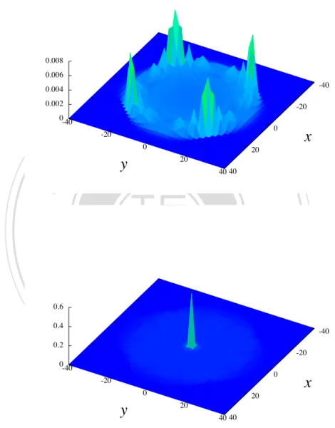
(42) Discrete-Time Quantum Walks. after 40 steps.. 立立. 政治大. •‧. •‧ 國. ㈻㊫學. n. er. io. sit. y. Nat. al. Ch. engchi. i Un. v. Figure 3.3: Spatial probability distribution for quantum walk on 2D lattice run for 40 steps with initial state given in Eq. (3.17) (top) and in Eq. (3.18)(bottom). Only even positions are shown, since odd positions have probability zero.. 32.

(43) 4 Continuous-Time Quantum 政治大 Walks 立立 •‧ 國. ㈻㊫學. The discrete-time version of quantum walks discussed in the previous chapter is only one way to introduce quantum e↵ects into random walks. Another route to. •‧. utilize quantum mechanics to move through graphs was introduced by Farhi and. y. Nat. and Gutmann [17], referred to as continuous-time quantum walk.. symmetric transition rate matrix M 8 > > dn , > < Mmn = , > > > :0,. n. al. can be represented by an N ⇥ N. er. io. G = (V, E) with constant transition rates. sit. Recall that a continuous-time classical random walk on an N -vertex graph. Ch. e nvgn =c vhmi. i Un. (vm , vn ) 2 E. v. (4.1). otherwise.. The probability distribution {Pn (t)} over the vertices {v1 , v2 , · · · , vN } at time t are the solution of the di↵erential equation @ Pn (t) = @t. X. Mnm Pm (t).. (4.2). m. We notice that this di↵erential equation is very similar to the Schrödinger equation i. @ | (t)i = H| (t)i, @t. 33. (4.3).

(44) Continuous-Time Quantum Walks. except that it lacks the factor of i. The key idea of Farhi and Gutmann [17] is to use the transition rate matrix as the generator of time evolution, i.e. as the Hamiltonian H. In this definition, the quantum walk on an undirected graph is obtained by replacing the di↵usion equation (4.2) with the Schrödinger equation. The set of vectors {|ni} associated with all vertices forms an orthonormal basis. for the Hilbert space. In the basis {|ni}, the Schrödinger equation describing the quantum walk is then written as i. X @ hn| (t)i = hn|H|mihm| (t)i, @t m. 立立. hn|H|mi = Mnm ,. (4.4). ㈻㊫學. •‧ 國. with. 政治大. (4.5). as given in Eq. (4.1). The solution of this di↵erential equation, known as the. •‧. probability amplitude, can be given in closed form as | (0)i,. y. Nat. iHt. (4.6). io. sit. hn| (t)i = hn|e. n. al. er. where the matrix exponential generated by the Hamiltonian corresponds to the time evolution operator. Ch. i iHt U.n. e nUg(t)c =hei. v. (4.7). Since the Hamiltonian is a Hermitian operator, this time evolution is unitary, U † U = I, and preserves normalization of the probability in the sense that @ X |hn| (t)i|2 = 0 . @t n Denoting the eigenvectors of H by |. ki. (4.8). and the corresponding eigenvalues by. Ek , the probability Pn!m (t) that the walker starting at t = 0 at site vn arrives on site vm at time t is given by Pn!m (t) = |hm|e. iHt. |ni|2 =. 34. X k. 2. e. iEk t. hm|. k ih. k |ni .. (4.9).

(45) 4.1 Continuous-time quantum walk on a line. Using the same notation for the quantum case (in fact, the eigenvalues and eigenvectors of the transition rate matrix M and the quantum Hamiltonian H are cl the same), the probability Pn!m (t) in the classical case is given by cl Pn!m (t) = hm|e. Mt. |ni =. X. e. Ek t. k. hm|. k ih k |ni.. (4.10). Since the eigenvalues Ek are non-negative (the matrix M given in Eq. (4.1) is nonnegative-definite), for t. 1 all exponential terms with Ek > 0 in the sum of. Eq. (4.10) decay to zero; the probability in the long time limit is then determined by the term with Ek = 0, leading to. 立立 lim P t!1. 政治大 1. cl n!m (t). =. N. .. (4.11). •‧ 國. ㈻㊫學. Unlike the classical case, the unitarity of the time evolution operator prevents. •‧. the probability for the quantum walk from a definite limit when t ! 1.. In principle, we could define a continuous-time quantum walk using any Her-. mitian Hamiltonian that respects the structure of the graph. For example, we. y. Nat. sit. could use the the adjacency matrix A of the graph, whose matrix elements Amn. er. io. are equal to one if vertices vm and vn are connected, and zero otherwise; although this matrix cannot be used as the generator of a continuous-time classical random. al. n. walk.. 4.1. Ch. engchi. i Un. v. Continuous-time quantum walk on a line. Let us first consider a quantum walk on an infinite integer line, with V = Z and nearest-neighboring edges. The Hamiltonian for this problem is defined by (cf. Eq. (2.26)) H|ni =. |n. 1i + |n + 1i. 2 |ni ,. (4.12). where the transition rate is set to . To obtain the probability amplitude hn + x|e. for the walk to move a distance x (2 N) in time t, one can actually simply use the analytic continuation t ! it of the exact result for the corresponding continuous. 35. iHt. |ni.

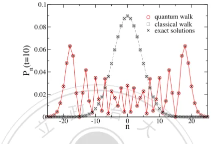
(46) Continuous-Time Quantum Walks. 0.1 quantum walk classical walk exact solutions. Pn(t=10). 0.08 0.06 0.04 0.02 0. 立立. -20. 政治大 n -10. 0. 10. 20. •‧. •‧ 國. ㈻㊫學. Figure 4.1: Probability distributions for continuous-time random walks (classical and quantum) on an integer line at time t = 10; the transition rate is = 1. The data sets denoted by squares and circles are obtained by diagonalizing the transition rate matrix M (of the classical random walk) as well as the Hamiltonian H (of the quantum walk) for a finite line with 801 vertices. The data are compared with the exact solutions given in Eq. (4.13) and in Eq. (4.14) for an infinite line. The grey dashed line is the Gaussian approximation for the classical case. er. io. sit. y. Nat. time classical random walk. In the classical version (discussed in Sec. 2.2), the. n. al. i Un. probability of moving a distance x in time t is. Ch. e n g c h2 it Px (t) = e. v. Ix (2 t),. (4.13). where Ix is the modified Bessel function of order x. By replacing t with it in Eq. (4.13), we obtain the amplitude hn + x|e. iHt. |ni = e. i2 t x. i Jx (2 t),. (4.14). and the corresponding probability hn + x|e. iHt. |ni. 2. = Jx (2 t). 2. (4.15). for the quantum walk. Here Jx (t) is the Bessel function of order x. Eq. (4.14). 36.

(47) 4.2 Exponential speedup by quantum walk. describes a ballistic propagation with speed 2 [26]; thus the quantum walk moves a distance proportional to t, which is quadratically faster than the classical random p walk in which x / t.. 4.2. Exponential speedup by quantum walk. We have seen that the behavior of a quantum walk can be dramatically di↵erent from that of its classical counterpart. In Ref. [27] a finite graph is given to demonstrate an even stronger example of the power of quantum walk, which will. 治政 The so-called glued trees graph G , studied in Ref. 大 [27], consists of two bal立立 anced L - level binary trees with the 2 leaves of the left tree identified with the be discussed in this section.. L L. •‧ 國. The number of vertices in GL is 2L+1 + 2L. ㈻㊫學. 2L leaves of the right tree according to the structure shown in Fig. 4.2 (for G4 ). 2. We are interested in the dynamics. of both the classical and quantum random walks from the leftmost vertex (the. •‧. root of the left tree) to the rightmost vertex (the root of the right tree).. y. Nat. It is not hard to see that a classical random walk on the graph starting from 1. Due to the. er. io. a considerable probability of reaching the right root for L. sit. the leftmost vertex will get trapped in the middle of the graph, and never has symmetry of the graph, it is more convenient to consider the probabilities, P` , for. n. al. Ch. i Un. v. the walker to be on each column indexed by ` = 0, 1, 2, · · · , 2L (starting from the. engchi. root of the left tree) while analyzing the dynamics of the walk. These probabilities at time t obey the di↵erential equations dP0 = 2 P0 + P1 dt dP2L = P2L 1 2 P2L dt 8 > > >2 P` 1 3 P` + P`+1 dP` < = P` 1 3 P` + 2 P`+1 > dt > > :2 P 2 P` + 2 P`+1 ` 1. for 0 < ` < L. (4.16). for L < ` < 2L for ` = L,. which are obtained by grouping the master equation for the probability at each vertex in the given column. The elements of the corresponding transition matrix. 37.

(48) Continuous-Time Quantum Walks. A. Column. B. 0. 政治大. 8 ! -2 -2 -2 -1 -1 -1 -1 Classical -1 -1 -1 -2 -2 -2 -2 2 3 3 3 3 3 3 3 ( 2 p p p p p p p p - 2 - 2 - 2 - 2 - 2 - 2 - 2 - 2 Quantum 2 3 3 3 3 3 3 3 2. 立立. 1. ) -2 -1. 2. 3. 4. 5. 6. 7. •‧. •‧ 國. ㈻㊫學. Figure 4.2: Glued trees graph G4 . The bottom panel shows the reduction to the column space for both the classical and quantum walks.. sit. y. Nat. al. er. io. are depicted in Fig. 4.2. The probabilities distribution over columns of G50 at. n. di↵erent time steps, obtained by solving this set of di↵erential equations with. Ch. the initial condition P` (t = 0) =. `,0 ,. i Un. v. are shown in Fig. 4.4 (a); the figure shows. engchi. that the probability accumulates rapidly in the middle of the graph, but the probability of reaching the right root evolves extremely slowly. As can be seen from Eqs. (4.16), in the left tree (0 < ` < L), the probability of moving from column ` to column ` + 1 is twice as great as the probability of moving from column ` to column `. 1; on the other hand, in the right tree (L < ` < 2L),. the probability of moving from column ` to column ` + 1 is half as great as the probability of moving from column ` to column `. 1. This asymmetry of the. probability implies that the probability of reaching column 2L in a time that is polynomial in L is exponentially small as a function of L. We now analyze the quantum walk on the glued trees graph, which is described. 38.

(49) 4.2 Exponential speedup by quantum walk. (a) Quantum. (b) Classical. 政治大. Figure 4.3: Comparison of the probability distributions at time t = 4 of continuous-time quantum walk (panel (a)) and classical random walk (panel (b)) starting from the left root of a glued trees graph G5 . It is evident that the spread of the quantum walk is faster than the analogous classical spread. The data obtained from our simulations are plotted using the software package qwViz [28].. 立立. io. sit. @ | (t)i = H| (t)i, @t. (4.17). er. Nat. i. y. •‧. •‧ 國. ㈻㊫學. by the Schrödinger equation. al. iv n C h e nspace 2)-dimensional Hilbert i U by all vertices, one deg c hspanned n. where the Hamiltonian is given by the transition rate matrix. Instead of working with the (2L+1 +2L. fines a (2L+1)-dimensional ”column subspace” spanned by the ”column-vectors” |c` i (where 0  `  2L) that are the equal superpositions of vertex-states on a given column `, that is 1 |c` i = p N`. X. n2 column `. |ni,. where N` is the number of the vertices in column ` and is given by 8 < 2` , 0  `  L, N` = :22L ` , `  `  2L. 39. (4.18). (4.19).

(50) Continuous-Time Quantum Walks. (a). 0 0.1 0.8. 35. 0.05. Pl. (b). 0.05. 15. 0 0.8 0.1. 0 0.6 0.1. 0 0.4 0.1. 0 0.6 0.1. 0 0.2 0.1. 0 0.4 0.1. 10. 0.2 20. 30. 0.4 40. 50. 0.6 60. column l. 70. 0.8 80. 90. 30. 0.05 0 0.2 0.1. 65. 0.05. 25. 0.05. 55. 0.05. 20. 0.05. 45. 0.05. 000. 0.1 1. 25. Pl. 0.1 1 0.05. 35. 0.05. 00. 100 1. 0. 10. 0.2 20. 政治大. (a) classical random walk. 立立. 0.1. 50. 0.6 60. column l. 70. 0.8 80. 90. 100 1. (b) quantum walk. 25. Pl. 0.05. 10. 20. 40. 50. Nat. column l. 70. 60. 80. 90. 100. io. er. (c) quantum vs. classical. sit. y. 30. •‧. 0 0. 0.4 40. ㈻㊫學. •‧ 國. (c). 30. Figure 4.4: Propagation in G50 starting at the left root. (a) Probability distribution P` (t) of a classical walk at time t = 25, 35, 45, 55, 65; (b) distribution of a quantum walk at time t = 15, 20, 25, 30, 35; (c) a comparison of the classical random walk and the quantum walk at time t = 25.. n. al. Ch. engchi. i Un. v. In this basis, the Hamiltonian has non-zero matrix elements given by hc` |H|c`±1 i =. p. 2 8 <2 , hc` |H|c` i = :3 ,. ` = 0, L, 2L. (4.20). otherwise.. The probability P` (t) of being on column c` with the initial condition P` (0) =. `,0. can be formally expressed as P` (t) = |hc` |e. 40. iHt. |c0 i|2 .. (4.21).

(51) 4.2 Exponential speedup by quantum walk. Denoting the eigenvalues of H by Ek and the eigenvectors of H by |. k i,. probability P` (t) is then given by |hc` |e. iHt. |c0 i|2 =. X. the. 2. e. iEk t. k. hc` |. k ih. k |c0 i .. (4.22). In Fig. 4.3(a) and Fig. 4.4(b) we show the numerical results for P` (t), obtained by solving the eigenvalue problem of H; the quantum walk shows a remarkable speedup of propagation through the glued trees, as compared with the classical random walk.. 政治大. 立立. 0.03. 0.03. io. (a) t = 100. 200. 0.03. 707. 400. 600. column l. 800. 1000. (b) t = 175. n. al. 0 0. 1000. y. Pl. Pl 800. sit. 600. column l. er. 400. 0.01. Nat. 200. 0.02. •‧. 0.01. ㈻㊫學. 0.02. 0 0. 495. •‧ 國. 283. Ch. engchi 0.03. v. 1000. Pl. 0.02. Pl. 0.02. i Un. 0.01. 0 0. 0.01. 200. 400. 600. column l. 800. 0 0. 1000. (c) t = 250. 200. 400. 600. column l. 800. 1000. (d) t = 354. Figure 4.5: Propagation in a large p graph G500 starting at the left root. The column located approximately at 2 2t is indicated by the red dashed line; this coincides with the location of the wavefront, implying that the wave packet propp agates with speed 2 2.. 41.

(52) Continuous-Time Quantum Walks. Indeed, by identifying the subspace of column-states |c` i, the quantum walk. on the L - level glued trees graph starting from the left root is e↵ectively the same as a quantum walk on a line with 2L + 1 vertices, with all edge weights the same (see Fig. 4.2, bottom panel). In the limit of L ! 1, the walk on GL is nearly. identical to a quantum walk on the infinite, translationally invariant line. The probability amplitude to go from column ` to column `0 for L ! 1 in a time t is then (cf. Eq. 4.14) hc`0 |e. iH. t|c` i = e. i3 t `0 `. i. p J`0 ` (2 2t),. (4.23). 政治大. being a Bessel function of order `0 `; this corresponds to propagap tion with speed 2 2 . To verify this, we numerically compute the probability with J`0. `. 立立. •‧ 國. •‧. Quantum walk on square lattices. sit. y. Nat. 4.3. ㈻㊫學. |hc` |e iHt |c0 i|2 for a large system with L = 500 and = 1 at t = 100, 175, 250 and 354. The results are shown in Fig. 4.5. The wavefront of the distribution at p t is located approximately 2 2 t away from the left root.. The quantum walk on the glued trees graph that we considered in the previous. io. n. al. er. section is e↵ectively a one-dimensional quantum walk problem. In this section, we. i Un. v. focus on continuous-time quantum walks on structures topologically equivalent to two-dimensional (2D) square lattices.. 4.3.1. Ch. engchi. The regular lattice. e = 2L + 1 sites per row or We first consider a 2D regular square lattice with L column. Each pair of nearest-neighbor vertices has an edge connecting them, and. each vertex has degree four. Periodic boundary conditions (PBC) are imposed in two directions; the lattice can then be thought of as being mapped onto the surface e2 vertices of the system of a three dimensional torus (or doughnut). The N = L. give rise to N orthonormal basis vectors, denoted by |ni, or |nx i ⌦ |ny i ⌘ |nx , ny i with nx , ny 2 [ L, L] being integer labels in x and y directions Without loss of generality, we set the transition rate. = 1 for every edge.. The continuous-time quantum walk is defined by the Hamiltonian given by the. 42.

(53) 4.3 Quantum walk on square lattices ↵ transition rate matrix. The Hamiltonian H acting on a state nx , ny reads ↵ ↵ H nx , ny =2 nx , ny. + 2 n x , ny. where we require. ↵. nx. 1, ny. n, ny. ↵ ↵ L + 1, ny ⌘ L, ny , ↵ ↵ nx , L + 1 ⌘ nx , L ,. ↵. 1. ↵. nx + 1, ny. ↵. ↵ n, ny + 1 ,. ↵ ↵ 1, ny ⌘ L, ny ↵ ↵ nx , L 1 ⌘ nx , L L. 政治大 1i |n + 1i ⌦ |n i. (4.24). (4.25). to fulfill the PBC. Eq. 4.24 can be written in a tensor product form as. 立立 |n. H |nx i ⌦ |ny i = 2 |nx i. x. x. •‧ 國. |ny. 1i. |ny + 1i. ㈻㊫學. + |nx i ⌦ 2 |ny i. y. ⌘ Hx |nx i ⌦ |ny i + |nx i ⌦ Hy |ny i. •‧. The Hamiltonian H is then decomposed into two parts. y. sit. io. n. al. C h |nx 1i |nx +U1in i Hy |ny i = 2 |ny i e |nyn g1ic h|ni y + 1i. Hx |nx i = 2 |nx i The eigenvectors, |. kx(y) i,. |. (4.27). er. Nat. H = Hx + Hy ,. corresponding to the operators for x and y components. (4.26). v. (4.28). of Hx(y) are the so-called Bloch states [30] given by nx =L 1 X p i = e kx e L nx = L. ny =L 1 X | ky i = p e e ny = L L. ikx nx. |nx i, (4.29). iky ny. |ny i,. e and ky = 2⇡`y /L, e with `x , `y = 1, · · · , L; e the corresponding where kx = 2⇡`x /L eigenvalues are. Ekx(y) = 2. 2 cos kx(y) .. 43. (4.30).

(54) Continuous-Time Quantum Walks. From Eq. (4.26), we find the eigenvalues Ek and the eigenvectors |. ki. for the full. Hamiltonian H: E k = E kx + E ky = 4 and |. ki = |. 2 cos kx. 1 X p i = e ky N nx ,ny. kx i ⌦ |. 2 cos ky. i(kx nx +ky ny ). (4.31). |ni .. (4.32). 治政大 from state |ni = |n , n i to expression for the probability amplitude of moving 立立 state |mi = |m , m i in time t:. Using the solution of the eigenvalue problem for H, we obtain the exact x. iHt. |ni =. 1 X e N k ,k x. i(4 2 cos kx 2 cos ky )t. e. ㈻㊫學. hm|e. y. ikx (mx nx ) iky (my ny ). ,. (4.33). y. •‧. •‧ 國. x. y. and the corresponding probability (denoted by Pn!m (t)) 2. |ni .. (4.34). n. er. io. al. iHt. sit. y. Nat. Pn!m (t) ⌘ hm|e. i Un. v. In the limit N ! 1, we may use a continuum approximation to rewrite the. Ch. engchi. expression in Eq. (4.33) to [31] hm|e. iHt. Z e i4t 2⇡ |ni ! 2 dkx e ikx (mx nx ) ei2t cos kx 4⇡ 0 Z 2⇡ ⇥ dky e iky (my ny ) ei2t cos ky =e. 0 i4t (mx nx ) (my ny ). i. i. Jm x. (4.35). nx (2t)Jmy ny (2t). where we have used an integral representation [29] 1 Jn (t) = 2⇡in. Z. 2⇡. d✓ ei✓n eit cos ✓ .. (4.36). 0. for the Bessel function Jn (t) of the first kind. The probability of moving from |ni. 44.

(55) 4.3 Quantum walk on square lattices. to |mi in a lattice of infinite size is then lim Pn!m (t) = Jmx. N !1. nx (2t)Jmy ny (2t). 2. (4.37). In Fig. 4.6 we show the probability distribution for quantum walk on a finite 2D lattice run for di↵erent time spans with the starting point at the origin (0, 0). Since the time evolution of the walk is governed by a separable Hamiltonian H = Hx + Hy with a separable initial condition, the di↵erent spatial dimensions behave independently; thus the probability at any t shows a symmetrical pattern. 政治大 (t), as a function of time立立 t, for various n for finite N = 513 .. along x and y directions.. To verify the results for an infinite lattice, we calculate the probabilities P0!n. 2. As shown. •‧ 國. ㈻㊫學. in Fig. 4.7, the data obtained from the Bloch ansatz are in excellent agreement with the exact solutions for N ! 1. Furthermore, the plots in Fig. 4.8 for a large lattice of size N = 10252 clearly show that the leading edge of the probability. •‧. distribution P0!n (t) of arriving at vertices |ni = |n, ni along the diagonal path. y. Nat. between the staring point |0, 0i and the corner vertex (L, L) moves approximately. er. io. infinitely large system.. sit. with speed 2; this is indeed implied in the exact expression (in Eq. (4.37)) for an Now we turn to the comparison with the classical random walk. Using the. n. al. cl i v (t) for the classical C hk i, the probabilityUPnn!m engchi. eigenvalues Ek and the eigenvectors | case can be calculated via. cl Pn!m (t) =. 1 X e N k. Ek t. hm|. k ih k |ni.. (4.38). We focus on the return probabilities Pr (t) ⌘ Pn!n (t) (for the quantum case) and cl Pr (t) ⌘ Pn!n (t) (for the classical case), which are the probabilities to be still or. again at the initial state at time t. A fast decay of the return probability implies a fast propagation through the graph since the probabilities (1. Pr (t)) to be at. any but the initial state grow quickly. In Fig. (4.9), we consider Pr (t) for the lattice size 33 ⇥ 33. As discussed before, for the classical random walk the long. cl time limit of the probabilities Pmn (t) reaches the equipartition value 1/N . In the. same way, the long time limit of the return probability Prcl (t) is given by 1/N . In. 45.

(56) Continuous-Time Quantum Walks. 立立. 政治大. •‧. •‧ 國. ㈻㊫學. n. er. io. sit. y. Nat. al. Ch. engchi. i Un. v. Figure 4.6: Time evolution of the probability distribution over the square lattice of size 65 ⇥ 65 with the initial state |nx = 0i ⌦ |ny = 0i.. 46.

(57) 4.3 Quantum walk on square lattices. 8. -4. P0n(t) . [10 ]. -4. P0n(t) . [10 ]. 3. 2. 1. 6. 4. 2. 30. t. 40. 10. 50. t. 20. 30. (b) |ni = |32, 16i 政治大 Figure 4.7: The probability for a large 2D square lattice of size N = 513 of arriving on vertex (a) |64, 16i 立立 and (b) |32, 16i with initial state |0, 0i, plotted as a (a) |ni = |64, 16i. 2. io. al. y. 64. 128. P0n(t). n. 0.004. 32. Ch. engchi. sit. 16. t=8 t = 16 t = 32 t = 64. er. Nat. 0.006. •‧. •‧ 國. ㈻㊫學. function of time t. The black line corresponds to data obtained using the Bloch ansatz; the orange dashed line indicates the exact solution for N ! 1, given in Eq. (4.37).. 100. 120. i Un. v. 0.002. 0 0. 20. 40. 60. n. 80. Figure 4.8: Propagation in a large lattice of size N = 10252 along a diagonal path starting at the middle vertex |0, 0i to the corner vertex (L, L). The vertex |n, ni located at 2t is indicated by the red dashed line, which is also the approximate location of the wavefront at time t.. 47.

(58) Continuous-Time Quantum Walks. 0. 10. -2. Pr(t). 10. quantum classical. -4. 10. -6. 10. 政治大. -8. 立立. -1. 10. 0. 1. 10. 2. 10. 10. ㈻㊫學. t. •‧ 國. 10. •‧. Figure 4.9: The return probabilities, Pr (t) and Prcl (t), for the quantum and classical random walks on a 2D lattice of size 332 . The blue dashed line, proportional to 1/t2 , indicates the decay behavior of the quantum probability in the intermediate range, where the classical probability decays as Prcl (t) ⇠ 1/t before it converges to Prcl (1) = 1/N. io. sit. y. Nat. er. contrast, the probability Pr (t) for the quantum case does not decay to a constant value at t ! 1, but oscillates over time. In the intermediate range (between. al. n. iv n C t ⇡ 0.5 and t ⇡ 100) the classical probabilityUdecays algebraicly as Prcl (t) ⇠ 1/t, heng chi while the quantum probability decays faster (Pr (t) ⇠ 1/t2 ) before it oscillates around the long time average.. 4.3.2. Bond percolation on the square lattice. Percolation models, introduced by Broadbent and Hammersley [32], are mathematical models of random media. The analysis of di↵usion (or transport) in higher dimensional disordered media by means of random walk on a percolation system was suggested by de Gennes [33], for which he coined the term ”ant in the labyrinth”. Consider the square lattice Z2 (infinitely large); each edge between two nearestneighbor vertices is present with probability p and absent with probability 1. 48. p.

(59) 4.3 Quantum walk on square lattices. (a) bond percolation. (b) site percolation. 政治大. Figure 4.10: Illustrations of (a) bond percolation and (b) site percolation on twodimensional square lattices with open boundary conditions. There are two clusters, denoted by red and blue, on each lattice.. 立立. •‧ 國. ㈻㊫學. [see Fig. 4.10(a)]. This model is called a bond percolation model (In analogy with the bond percolation model, one defines the site percolation model in which. •‧. vertices (sites) are randomly removed with probability 1. p [see Fig. 4.10(b)]).. y. Nat. A ”cluster” on this graph is a set of connected vertices. As the occupation prob-. sit. ability, p, is increased from zero, the average or typical clusters become larger,. al. er. io. both in terms of the number of vertices (mass) and geometric size. The graph is. n. said to be ”percolate” if there is an infinite cluster containing the origin; if the. Ch. i Un. v. graph is translation-invariant there is no di↵erence between the origin and any. engchi. other vertex. There exists a critical value pc (called the percolation threshold ) for the occupation probability p such that all clusters in the graph are finite when p < pc , but there exists an infinite cluster when p > pc . The change in behavior while crossing the percolation threshold is an example of a phase transition. For the square bond percolation the percolation threshold is exactly known, pc = 1/2 [34]. On a finite lattice, ”infinite clusters” defined above correspond to spanning clusters that touch opposite boundaries. This assumption is valid for large lattice sizes and preferably when periodic boundary conditions are imposed. The dilute lattice provides a constrained arena for random walk. The random walker (the ”ant”) can only move within a cluster, but not move between disjoint clusters. There are two interesting aspects for studying random walk in percolation. First, percolation graphs are quenched disordered media for random. 49.

(60) Continuous-Time Quantum Walks. (a) p = 0.49. (b) p = pc = 0.50. (c) p = 0.51. 政治大. Figure 4.11: Phase transition in bond percolation on a two-dimensional square lattice of size 512 ⇥ 512 with periodic boundary conditions. Only the largest cluster at each occupation probability p is shown. A cluster that spans to opposite boundaries (a percolating cluster) appears only at p pc .. 立立. •‧ 國. ㈻㊫學. walks. Second, percolation clusters at p  pc are fractal objects1 ; they are irreg-. ular geometric objects with an infinite nesting of structure at all scales and with. •‧. noninteger dimensions; for example, at pc , the mass M of the largest cluster scales. y. Nat. with the linear lattice size (L) as M ⇠ Ldf , with df = 91/48 for two dimensions. sit. [34]. Both randomness and fractal contribute anomalous di↵usion in percolation;. n. al. er. io. the time dependence of the mean square displacement becomes. Ch. i Un. [hr2 i]av ⇠ t2/dw. engchi. v. (4.39). with dw > 2 [36, 37], where [ · ]av denotes an average over di↵erent disorder real-. izations. We note that the slowdown of the random walk in a higher dimensional random medium is in general less pronounced than the slowdown in 1D, where a logarithmically slow di↵usion is observed (see Sec. 2.1.2). A heuristic explanation for such a di↵erence with the 1D case is that due to a less restricted topology of space in higher dimensions, it is much harder to force the random walk to visit traps. Unlike a classical random walk which is essentially a di↵usion process, a quantum walk manifests quantum coherences, which can lead to faster spreading, as 1. A fractal is a mathematical set that has a fractal dimension that usually exceeds its topological dimension. A fractal is not smooth at every point. Mandelbrot [35] coined the term ”fractal” to describe the property of being fractured at every point.. 50.

量子模擬: 量子隨機行走法則 與 量子退火式最佳化演算 - 政大學術集成

量子模擬: 量子隨機行走法則與量子退火式最佳化演算 - 政大學術集成