應用於2.5D環境以粒子過濾演算法與感測元件輔助的無線定位系統

國

立

交

通

大

學

資訊科學與工程研究所

碩

士

論

文

應用於 2.5D 環境以粒子過濾演算法與感測

元 件 輔 助 的 無 線 定 位 系 統

Wireless Location Tracking by a Sensor-Enhanced

Particle Filter in 2.5D Buildings

研 究 生：朱瑞浩

應用於 2.5D 環境以粒子過濾演算法與感測元件輔助的無線定位系統

Wireless Location Tracking by a Sensor-Enhanced Particle Filter in 2.5D Buildings

研 究 生：朱瑞浩 Student：Jui-Hao Chu

指導教授：曾煜棋、易志偉 Advisor：Yu-Chee Tseng、

Chih-Wei Yi

國 立 交 通 大 學

資 訊 科 學 與 工 程 研 究 所

碩 士 論 文

Submitted to Institute of Computer Science and Engineering College of Computer Science

National Chiao Tung University in partial Fulfillment of the Requirements

for the Degree of Master

in

Computer Science

June 2009

Hsinchu, Taiwan, Republic of China

應用於 2.5D 環境以粒子過濾演算法與感測元件

輔助的無線定位系統

學生：朱瑞浩

指導教授：曾煜棋 教授

易志偉 教授

國立交通大學資訊科學與工程學系研究所

摘

要

在室外空曠環境，GPS 具有不錯的定位結果，目前，如何得到使

用者在室內環境的位置，受到廣泛的討論和研究，其中尤其以基於無

線電訊號強度的樣本比對演算法具有最好的定位結果，但是其最大的

缺點在於，無線電訊號先天上容易受到環境影響，導致訊號強度飄移

的問題，造成定位結果產生誤差，同時，過去的研究，鮮少討論多層

樓等室內立體定位環境 (2.5D 環境)，因此，在此篇，我們為無線電

訊號強度樣本比對演算法提出了應用於 2.5D 定位環境的 SEPF

(sensor-enhanced particle filter) 模 型 ， 透 過 慣 性 感 測 元 件 (IMU

sensors) 感測使用者的移動軌跡，藉以調整粒子 (particles) 的位置分

佈和權重值 (weight)。在此篇中，我們會介紹如何建構室內定位環境

的 2.5D 模型，並且在此模型中，粒子的實際取樣 (sampling) 與重新

取樣 (re-sampling) 的實作方式，以及藉由分析慣性感測元件的感測

值來估測使用者目前的移動行為，例如行走於路面上或樓梯、搭乘電

梯等，透過慣性感測元件來克服無線電訊號強度飄移的問題。最後利

用我們開發的定位系統雛形，驗證我們的系統效能。

關鍵字: 慣性感測元件，定位系統，粒子演算法，遍佈計算，感測

網路。

Wireless Location Tracking by a

Sensor-Enhanced Particle Filter in 2.5D

Building

Student：Jui-Hao Chu

Advisors：Dr. Yu-Chee Tseng

Dr. Chih-Wei Yi

Institute of Computer Science and Engineering

National Chiao Tung University

ABSTRACT

For outdoor localization, GPS already provides a satisfactory solution.

For indoor localization, however, a globally usable solution is still

missing. One promising direction is the pattern-matching solution that

relies on RF signals from existing network infrastructures. One major

drawback of such systems is the signal-drifting problem, which is an

inherent physical constraint. Also, most works only consider single-floor

buildings. However, buildings normally have multiple floors (i.e., of 2.5

dimensions). This paper proposes a SEPF (sensor-enhanced particle

filter)} model for RF-based pattern-matching localization in a 2.5-D

building. IMU sensors are adopted to capture human mobility, while

particles reflect the belief on where the user is located. Our framework

addresses the following important issues. First, our 2.5-D building model

considers multiple floors connected by stairs and elevators. Second, we

show how particles should be sampled/re-sampled in a 2.5-D building to

reflect change of brief. Third, IMU sensor inputs are exploited to conquer

the signal-drifting problem and to predict user's behaviors (walking on

grounds/stairs and taking elevators). A prototype has been developed and

intensively tested to verify the model.

Keywords: IMU (inertial measurement unit), location tracking, particle

filter, pervasive computing, sensor network.

誌

謝

首先，誠摯的感謝我的兩位指導教授，曾煜棋以及易志偉

教授，在這兩年持續的指導和鼓勵，在這段時間中碰到許多

困難，但是只要多與老師們請教，都可以迎刃而解，所以非

常感謝兩位老師，幫助我得以完成這篇論文。

接著，我要感謝我們小組的學長，羅棨鐘、郭聖博兩位學

長，在研究上，給我許多建議和指導。並且我也要感謝實驗

室所有的同學，在這段時間的相互關心和幫助。

最後，我要感謝我的家人，不僅栽培我，並且在這段時間

給我許多鼓勵和支持。

Contents

1 Introduction 1

2 Preliminaries 5

2.1 Bayes and Particle Filters . . . 5

2.2 IMU Sensors . . . 6

2.3 2.5-Dimensional Building Model . . . 10

3 Sensor-Enhanced Particle Filter for 2.5D Location Tracking 14 3.1 Behavior-Predicting Module . . . 16

3.1.1 Horizontal Motion Detection . . . 16

3.1.2 Stair Motion Detection . . . 20

3.1.3 Elevator Motion Detection . . . 20

3.2 Particle-Sampling Module . . . 21

3.3 Particle Filtering Module . . . 25

3.3.2 The Passing Wall Filtering . . . 26 3.4 Particle Weighting Module . . . 27 3.5 Particle ReSampling Module . . . 28

4 Simulation Environment and Results 30

4.1 Singal Path Loss Models . . . 31 4.2 The Impacts of System Parameters . . . 34

5 System Implementation 38

List of Figures

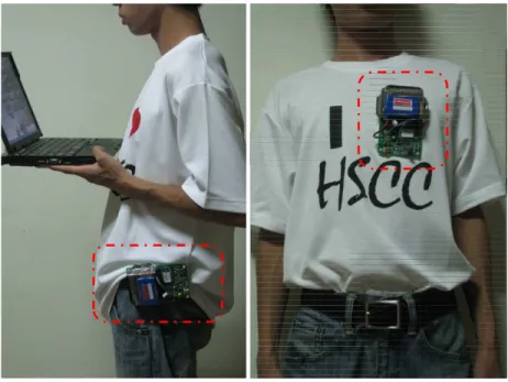
2.1 mounting sensor device on waist or hanging on chest. . . 7

2.2 from moving state to halting state. . . 8

2.3 walking on grounds. . . 8

2.4 walking on a circle. . . 8

2.5 going up/down stairs. . . 9

2.6 going up/down an elevator. . . 9

2.7 2.5-D Building Model. . . 11

2.8 The Subgraphs of 2.5-D Building Model. . . 12

3.1 The SEPF architecture. . . 15

3.2 An illustration of the horizontal and vertical motion prediction. . . 17

4.1 An illustration of the simulation environment. . . 31

4.2 An impact of theAP s. . . 35

4.3 An impact of noise deviation with training grain size. . . 35

4.5 An impact ofW AF . . . 36 4.6 An impact of estimating dynamic ofIMU Sensors. . . 37

Chapter 1

Introduction

Location-based services LBSs have been regarded as a killer application in mo-bile networks. A key factor to its success is the location estimation accuracy. For outdoor localization, GPS already provides a satisfactory solution. For in-door localization, however, a globally acceptable solution is still missing. Many indoor localization technologies have been proposed, such as infrared-based [4], ultrasonic-based [10], and RF-based systems [2]. Generally, localization mod-els can be classified as AoA-based [8], ToA-based [1], TDoA-based [11], and fingerprint-based [2][7][9].

In this work, we are interested in the pattern-matching localization method, such as RADAR [2]. This method does not rely on calculating signal fading in an environment. Instead, it relies on a training phase to collect the radio signal strength (RSS) patterns at a set of training locations from pre-deployed beacons

into a database (called radio map). These beacons can be existing infrastructures, such as IEEE 802.11 access points, GSM base stations, or a sensor network. Then, during the positioning phase, an object to be localized can collect its current RSS pattern and compare it against the radio map to predict its location.

The pattern-matching solutions have three main drawbacks. First, its train-ing process is very labor-intensive, especially in a large-scale field. Second, it suffers from the signal-drifting problem; the radio maps measured earlier may significantly deviate from the current ones. Third, most works are limited to 2-D sensing fields (e.g., a single-floor building). However, buildings normally have multiple floors. The first issue has been studied in [13], the second in [17][16], but the last one has been rarely addressed.

This paper proposes a SEPF (sensor-enhanced particle filter) model for RF-based pattern-matching localization in a 2.5-D building. IMU sensors are adopted to capture human mobility patterns, while particles help reflect our belief on where the user might be located. Our framework addresses the following important is-sues. First, our 2.5-D building model considers multiple floors connected by stairs and elevators. Second, we show how particles should be sampled/re-sampled in a 2.5-D building based on sensor inputs to reflect change of belief. Third, IMU sensor inputs are exploited conquer the signal-drifting problem and to predict hu-man’s main indoor behaviors (such as halting, walking on grounds, going up/down stairs, and taking elevators). A prototype has been developed and intensively

tested to verify our model.

Particle filters are sample-based implementation of Bayesian filters using a set of samples, i.e., particles, to reflect the probability densities of our belief [6]. In the scope of indoor localization, it estimates locations by recursively calculating current probability distributions based on measurements of current observation. The key components of Bayesian filter are observation, prediction, and history models. The observations could be from sensors or mathematical models. The-oretically, it can be applied to most positioning algorithms as long as we have some sort of prediction on user mobility. For example, a tracking system can exploit mobility history to conjecture user’s trajectory [3]. For pattern-matching solutions [14], RSSI is the only observation used to represent its belief about a dynamic system at time t as a probability distribution over the state space. The parameters and noise components of particle filters can be estimated from training data or tuned manually.

Hence, we propose a SEPF architecture with particle filter to obtain the ac-tual mobility model. And then, using mobility model to predict the propagation of particles. Traditionally, the real time mobility model can not directly get from users, but we presently utilize the sensor to achieve it. According to our study, the observation model also conforms to the model of the fingerprint base posi-tioning algorithm [5]. The philosophy of particle filter conforms to the tracking positioning algorithm by consulting history. And, the real time mobility model is

appropriate for adding the prediction model of it. Based on the mobility model, we can get better in positioning, because the particles are distributed around the true user‘s positioning location [15]. Therefore, we propose a positioning algorithm based on particle filter involving changeable mobility model.

The rest of this paper is organized as follows. Chapter 2 gives some prelimi-naries. Chapter 3 describes our SEPF architecture. Performance figures are pre-sented in Chapter 4. Chapter 5 introduces our prototyping details and experiment results. Finally, Chapter 6 concludes this paper.

Chapter 2

Preliminaries

2.1

Bayes and Particle Filters

Bayes filters probabilistically estimate a dynamic system’s state from observa-tions that could be disturbed by noise. In pattern-matching localization, the state could be a person’s location and the observations are RSS patterns. Bayes filters represent the state at timet by a random variables xt. It establishes a probability

distribution over xt, called belief Bel(xt). The goal is to sequentially estimate

such beliefs over the state and time spaces. Specifically, let the sequence of time-indexed observations bez1,z2,. . ., zt. Bel(xt) is defined by the posterior density

of statextconditioned on all previous observations:

The belief answers the question: “What is the probability that the person is at loca-tionxtif the sequence of observations isz1,z2, ...,zt?” In general, the complexity

to compute Bel(xt) grows exponentially over time. To make the computation

tractable, Bayes filters assume that the dynamic system is Markovian in that the current statextcontains all relevant information. So states beforext−1provide no

additional information. In our localization example, this means that we only need to work on the relation betweenxt−1andxt.

To realize different density functions ofxt, particle filters represent beliefs by

a set of samples, or particles:

Bel(xt) = St= {< x

(i)

t , w

(i)

t > |i = 1, ..., n}, (2.2)

where, each x(i)t is a state and w (i)

t is its weight. These w (i)

t s sum up to one.

Particle filters realize Bayes filters by a sequence of sampling, weighting, and resampling procedures. Its key advantage is the capability to represent arbitrary density functions, even in non-Gaussian, non-linear dynamic systems. It allows us to focus on resources (particles) in state spaces with high probabilities.

2.2

IMU Sensors

We are interested in using IMU (inertial measurement unit) sensors to capture typical human mobility patterns inside a building. We consider four main mobility patterns: halting, walking on grounds, going up/down stairs, and taking elevators.

Figure 2.1: mounting sensor device on waist or hanging on chest.

Mobility patterns will be tracked by a triaxial accelerometer (g-sensor), which can report 3D accelerations, and an electronic compass, which can report the angle relative to north.

The g-sensor combines three angular rate gyros with three orthogonal DC ac-celerometers and three orthogonal magnetometers to output its orientation in dy-namic and static environments. The outputs of them are rate of rotation, quantity of gravity and quantity of gauss. The size of it is 64 millimeter by 90 millimeter and 25 millimeter. And, the gravity is 75 grams with enclosure. Based on the official specifications, the accuracy of the orientation is about 0.5 degree for static test conditions and 2.0 degree for dynamic test conditions.

0.06 0.04 0.02 0 0.02 0.04 0.06 0.08 Acceleration Standing halting walking 0.06 0.04 0.02 0 0.02 0.04 0.06

Sitting (on sofa)

halting walking 0.06 0.04 0.02 0 0.02 0.04 0.06 0.08

Sitting (on wheel chair)

halting walking

Figure 2.2: from moving state to halting state.

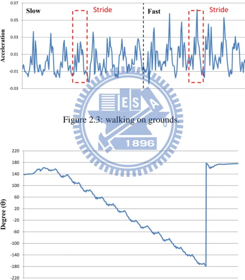
0.03 0.01 0.01 0.03 0.05 0.07 Acceleration Stride Stride Slow Fast

Figure 2.3: walking on grounds.

220 180 140 100 60 20 20 60 100 140 180 220 D eg ree ( )

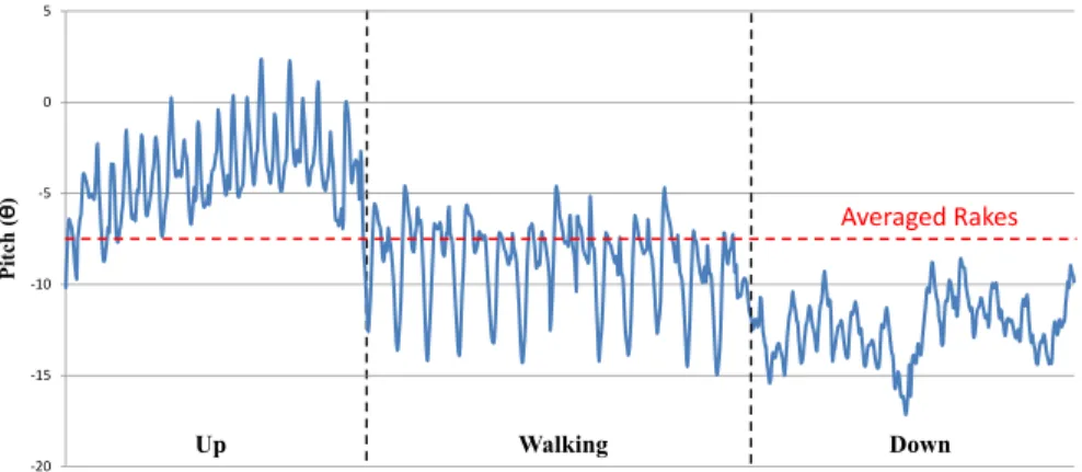
20 15 10 5 0 5 P it ch ( ) Up Walking Down Averaged!Rakes

Figure 2.5: going up/down stairs.

0.05 0.04 0.03 0.02 0.01 0 0.01 0.02 0.03 0.04 Up 3 floor 0.05 0.04 0.03 0.02 0.01 0 0.01 0.02 0.03 0.04 Up 2 floor 0.04 0.03 0.02 0.01 0 0.01 0.02 0.03 0.04 Acceleration Up 1 floor

Figure 2.1shows two ways to mount sensors devices on a human body in our experiment. Figure 2.2shows the outputs of a g-sensor when a person transits form a moving state to a halting state. Figure 2.3shows the outputs of a g-sensor when a person walks on grounds. Figure 2.4shows the outputs from an electronic compass when a person walks in a circle of radius 2m. Figure 2.5shows the outputs of a g-sensor when a person goes up/down stairs. Figure 2.6shows the outputs of a g-sensor when a person goes up/down an elevator.

As can be seen, these patterns all have their special features that can be easily recognized.

2.3

2.5-Dimensional Building Model

We now develop a graph-like model to represent a 2.5-D building. The repre-sentation facilitates us to describe how particles flow around a building in the yet-to-be-presented indoor localization scheme. We are given the floor plans of a 2.5-D building. Each floor may have rooms, partitions, hallways, etc. Floor is connected by stairs and elevators. The graph is denoted byG = (V, E). A vertex

in V could be one partition unit on a floor, a stairway, or an elevator. An edge

in E connects two vertices in V by specifying the passable part between them.

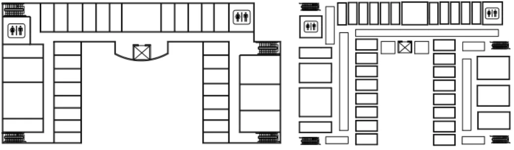
Figure 2.7(a) shows a floor plan of the Engineering Building III at NCTU, where our experiments are conducted.

Up

Up

Up Up

(a) 3f, Engineering Building III, NCTU.

4250.5 7 Up Up Up Up

(b) Partitioning of a floor plan.

Figure 2.7: 2.5-D Building Model.

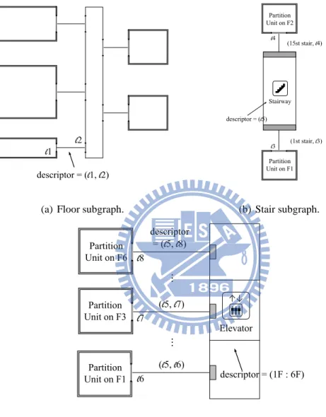
Given a building’s floor plan, we first deal with each floor by dividing it into multiple partition units. Each partition unit should be a convex polygon. Note that a convex polygon has the property that the line segment connecting any two points inside must fall inside the polygon itself; from particle filters’ prospect, this means that it allows a particle to move in a straight line between these two points. Figure 2.7(b) shows an example. Between two partition units, there are passable and impassable parts. Each passable part is represented by an edge inE together with a descriptor to specify the line segment of the two corresponding polygons constituting the passable part. From particle filters’ prospect, these passable parts are pathways for particles to flow around. Excluding passable parts, the rests are impassable parts, which particles are not allowed to cross over. Figure 2.8(a) shows how we construct partition units. Note that the labels on edges are their descriptors (for passable parts).

l l l

l

(a) Floor subgraph.

l l l l l (b) Stair subgraph. Ξ Ξ l l l l l l l l l (c) Elevator subgraph.

specify the number of stairs inside. A stairway connects two floors and we use two edges inE to represent such relationships. Each edge connects the stairway to a partition unit of a floor and it two descriptors: (i) the stair that the partition unit is connected and (ii) the passable part in the partition unit. Figure 2.8(b) shows how we abstract such concepts.

Each elevator is also represented by a vertex and it has two descriptors: (i) the range of floors that it moves to and (ii) the polygon of its ground part. Note that for (i), it is not necessary for the elevator to be stop at each floor within this range. we use the same number of edges equal to the number of floors that the elevator stops to denote this. Each edge connects the elevator to a partition unit of a floor and it also has a descriptor to specify the passable parts of the partition unit and its own ground part. Figure 2.8(c) shows an example.

Chapter 3

Sensor-Enhanced Particle Filter for

2.5D Location Tracking

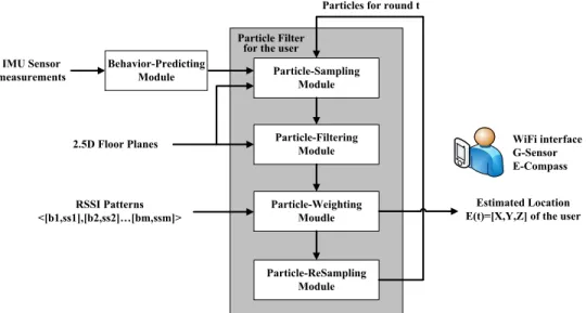
We propose a SEPF model for location tracking in a 2.5D building. We assume that the building has been deployed with some WiFi APs and a pattern-matching localization system is available. Figure 3.1 shows our SEPF work flow. It takes IMU sensor measurements, RSS patterns, and floor planes of a2.5D environment as inputs to predict users’ locations. Each user has to carry a WiFi interface, tri-axial accelerometer, and an electronic compass. The wireless interface can collect the RSSIs of its surrounding wireless beacons and the IMU sensors measurements and report to the PF to compute the user’s location. Users can only move on floor surfaces or go up/down stairs/elevators. The 2.5D building model defined in Sec. 2.3 is used.

Particle-Sampling Module Particle-Filtering Module Particle-Weighting Moudle Particle-ReSampling Module Behavior-Predicting Module IMU Sensor measurements 2.5D Floor Planes RSSI Patterns <[b1,ss1],[b2,ss2]…[bm,ssm]> Estimated Location E(t)=[X,Y,Z] of the user Particles for round t

Particle Filter for the user

WiFi interface G-Sensor E-Compass

Figure 3.1: The SEPF architecture.

Like typical PFs, our architecture also has sampling, particle-weighting, and particle-resampling modules. In addition, we add two new mod-ules: behavior-predicting and particle-filtering modules. The behavior-predicting module collects the IMU sensor outputs to predict the user’s current mobility pat-tern. The prediction, together with the floor planes, helps the particle-sampling module to propagate particles. Then those particles with low credibility will be filtered out by the particle-filtering module according to the floor planes. Using the RSSIs, the particle-weighting module will assign weights to particles. It also produces the estimated location of the user. Finally, the particle-resampling mod-ule re-generates particles for the next round.

3.1

Behavior-Predicting Module

Based on floor plans and IMU sensor measurements, the behavior-predicting mod-ule estimates the user’s current motions. This improves over traditional PFs, which usually adopt a random model in sampling particles. This module gen-erates three outputs: _{H(t), S(t), and E(t). H(t) = {(t}i, di), i = 1, ..., ∞} is

a series of horizontal motion vectors, ti is the timestamp anddi is the

displace-ment vector on the xy-plane measured between time interval (ti−1, ti]. S(t) =

{(ti, si), i = 1, ..., ∞} is a series of stair motions, where ti is a timestamp and

si is the estimated number of stairs that the user has taken during time interval

(ti−1, ti] (we use 0 to mean “no stair motion”, and a negative/positive integer to

means how many stairs down/up). _{E(t) = {(t}i, ei), i = 1, ..., ∞} is a series of

elevator motions, wheretiis a timestamp andei is the estimated number of floors

that the user has taken during time interval (ti−1, ti] (we use 0 to mean “no

ele-vator motion”, and a negative/positive integer to mean how much floor down/up). Below, we discuss how these series are computed in our model.

3.1.1

Horizontal Motion Detection

The horizontal motion detection module is pedometer-based. A pedestrian’s hor-izontal motion is composed of a series of stepping events. In other words, the displacement vectordiis corresponding to a stride. The readings of the

eter is used to detect stepping, estimate each stride length, and also decide walking directions by the helping of the magnetometer.

Stepping Detection: The readings of the accelerometer are decomposed into

two vertical components and a horizontal components. We observed that each step incurs a pulse waveform in the vertical components. A pattern matching technique is used to detect pulse for counting steps. To improve the accuracy, the amplitude and duration of each pulse and the magnitude of horizontal components are used to filter out false detections. In average, the pedometer has an accuracy around 96%.

Stride Length: After a stride is detected, two featuresA and X are extracted from the pulse where A is the sum of the magnitude of the left slope and right slope andX is the norm of the first component of the discrete Fourier transform of the pulse. We use quadratic regression to estimate the stride length. In other words, the stride length is estimated by the following formula

aX2+ bXA + cA2+ dX + eA + f. (3.1)

The constantsa, b, c, d, e, f are obtained by the least square method.

Walking Direction: The horizontal components tend to parallel with the

walking direction. Therefore, we classify horizontal components into two groups, forward vectors and backward vectors. Forward vectors are roughly in the walking direction and backward vectors are roughly in the opposite directly. To determine

the walking direction, we sum forward vectors with the inverse of backward vec-tors. The sum vector is used to represent the walking direction. Then, to with the readings of the magnetometer, we can know the absolute walking direction (in the earth frame).

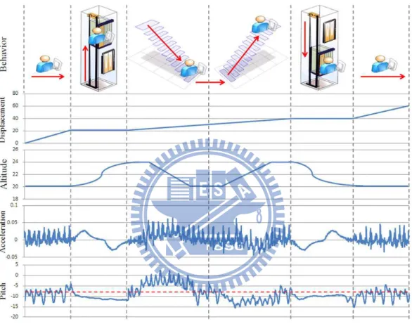
Figure 3.2 shows an example, where an user moves over around the indoor environment. The user starts at first floor and moves up to 3th floor by elevator. Then, user goes down to the first floor and returns to 3th floor by stair. In the end, user goes back to the first floor. Our goal is to generate the output H(t), where each di is a displacement vector that user has moved from ti−1 to ti. We

assume ti is a periodic event. Between ti−1 to ti, the stride events may occurj

times, name as −→di,j. We detect each stride event by capturing the sine wave from

acceleration and estimate stride length by integrate each sine wave as −→di,j. The

directionθ is represented by the angle measured in counterclockwise to the North Pole. If−→di,j andθ respectively denote the stride length and direction of a step, the

displacement vector can be obtained by the formula

3.1.2

Stair Motion Detection

The stair motion detection module is also pedometer-based. In our system, the typical value of the stair count si is ±1. S(t) = {(ti, ei)} is a discrete-time

sequence to represent whether the user has walked up/down stairs and, if so, how many stairs the user has gone. Since the event of one step up/down a stair can only be determined after the completion of the step, the reporting sequenceS(t) is always posterior.

Specifically, we will periodically look at the sensor measurements and attach a report toS(t) with a period of p. (The recommended p is around 2˜4 seconds.) At any pointt′

when an observation is made, we will merge the output from our step detector and the corresponding rake value. The rake value can be retrieved from the z-axis output of the g-sensor. A report of (t′

, k) will be attached to the sequence S(t), where k is the number of stair-up/stair-down events that are detected during the interval(t′

−p, t′

] (note that k should include the stair-up/stair-down event, if any, that was not reported at timet′

− p).

3.1.3

Elevator Motion Detection

Depending on the measurements from the g-sensor, we need generate E(t) =

{(ti, ei)}. E(t) is a discrete-time sequence to represent whether the user has taken

num-ber of floors that a user has moved can only be determined after the completion of signal changes has been observed and an elevator event normally takes 3 to 20 seconds, the reporting sequence E(t) is sometimes periodical and sometimes aperiodical. For this reason, the report of an elevator event is always posterior.

Specifically, we will periodically look at the measurements of the g-sensor in

the z-axis with a period of p. (The recommended p is around 1˜5 seconds.) Let

the output of the g-sensor at thez-axis over time be gz(t). At any point t′ when

we make an observation, we will conduct a curve-fitting ongz(t) for the part right

before t′

. If no curve in gz(t) matches with any of the curves representing an

elevator event as shown in Figure 2.6, a report of (t′_{, 0) will be attached to the}

sequenceE(t). Otherwise, if a match is found, let t′′

be the time point when the elevator event ends in the curve gz(t). A report of (t′′, k) will be attached to the

sequenceE(t), where k is the number of floors that the user has gone up/down (a positive value means “up” and a negative one means “down”). Also, in the later case, we will adjust the offset of our periodical reports to t′′

(i.e., the upcoming reports will be adjusted tot′′

+ p, t′′

+ 2p, etc.).

3.2

Particle-Sampling Module

The particle-sampling module takes three inputs: (1) the particles from the previ-ous round, (2) the sequences H(t), S(t), and E(t), and (3) the floor plans. This

module will adjust the location of each of these particles. Lettabe the timestamp

of the previous event that was processed and_{Pi(ta)} be the set of particles at ta.

Each particle Pi(ta) is associated with three descriptors: Pi(ta).par, Pi(ta).loc,

andPi(ta).wt. The partition unit and the location in the partition unit Pi(ta) is

lo-cated are written as Pi(ta).par and Pi(ta).loc, respectively. The weight of Pi(ta)

is written asPi(ta).wt. Given H(t), I(t), and E(t), we retrieve those unprocessed

events one-by-one according to their timestamps. We start from the unprocessed eventε with the earliest timestamp. Then we relocate each Pi(ta) according to the

following rules:

• Case 1: If Pi(ta).par is a partition unit on some floor, there are three cases.

1. If_{e ∈ H(t), let ε = (t}b,−→d ). We place {Pi(ta)} at the location:

Pi(tb).loc (t) = Pi(ta).loc (t) +−→d +−→R , (3.3)

where−→_{R = r · (cos θ, sin θ) is a 2D random vector, where r is a scalar} randomly selected from the interval[0, rmax] and θ is a angle randomly

selected from[0, 2π]. Here,−→d represents the displacement vector that is detected from IMU sensors. However, to accommodate the exis-tence of noise,−→R is to add some randomness to the new location of

Pi(tb). Note that if Pi(tb) remains in the same partition unit as Pi(ta),

we let Pi(tb).par = Pi(ta).par; otherwise, we let Pi(tb).par be the

perhaps due to noise, is whenPi(tb) falls outside the current floor. In

this case, we letPi(tb) be located at the point when it first moves out

of the boundary of the floor during the above movement.

2. if _{ε ∈ S(t), let e = (t}b, s). We first check if Pi(ta).loc is nearby

any passable part of a stairway. If so, we move this particle into this stairway. Specifically, if s = +1 and the distance from Pi(ta).loc

to any passable part of a stairway sw is within δf2s and the stairway

connects the current floor to a higher floor, we let Pi(tb).par = sw

andPi(tb).loc = 1. Similarly, if s = −1 and distance from Pi(ta).loc

to any passable part of a stairway sw is within δf2s and the stairway

connects the current floor to lower floor, we letPi(tb).par = sw and

Pi(tb).loc = −1. If none of those two cases sustain, Pi(tb) will remain

at the same partition unit and location asPi(ta).

3. if _{ε ∈ E(t), let e = (t}b, e). We check if Pi(ta).loc is nearby any

passable part of an elevator. If so, we move this particle into this elevator. Specifically, if e = “U′′

and the distance from Pi(ta).loc

to any passable part of an elevator ev is within a threshold δf2e, we

letPi(tb).par = ev and Pi(tb).loc = k+, wherek is the current floor

number and the superscript “+” means that the elevator is going up. Similarly, ife = “D′′

part of an elevatorev is within a threshold δf2e, we letPi(tb).par = ev

and Pi(tb).loc = k−, where k is the current floor number and the

superscript “-” means that the elevator is going down. If none of these two cases sustain, Pi(tb) will remain at the same partition unit and

location asPi(ta).

• Case 2: If Pi(ta).par is a stairway, there are two cases.

1. If the input is H(t) or E(t), we ignore that.

2. If the input is S(t), the particlePi(t).loc goes up/down by the estimated

number of stairssi. Also, a random movement is needed to disturb the

particles. If the new Pi(t).loc belongs to the first/last n stairs and its

trend is up/down, the particlePi(t).obj changes to floor and Pi(t).loc

goes to the boundary of the floor that connected with the stairs.

• Case 3: If Pi(ta).par is an elevator, there are two cases.

1. If the input is H(t), S(t), or , the begin event of E(t) we ignore that. 2. If the input is the end event of E(t), the particle moves to the floor

that belong to the estimated number ofsi. For example, if the input

isE(t) = (t1, +3), actually we may move from 3th floor to 6th floor,

Pi(t).obj will change to 4th, 5th, and 6th with a probability

with the elevator.

In the above discussion, we did not address how to assign weights to particles. Here we assume that each particle will inherit its previous particle’s weight, i.e.,

Pi(tb).wt = Pi(ta).wt.

3.3

Particle Filtering Module

Generally, the sampled particles are weighted directly in weighting module. It only uses the pattern matching scheme to figure out the location having the highest possibility from the particle with maximum weight. Intuitively, the precision will be gained if we took additional information of user into account for decision. Therefore, the particle filtering module utilizes the speed of user and floor plans to filter out the sampled particles that they are incredible.

3.3.1

The Speed Filtering

The speed filtering is used to adjust the coverage of particles. It restricts the par-ticles be spread on a radius of confident sizec which‘s center is the last estimated result with mobility shift. The particles which are outer this range will be filtered. The mobility shift is the displacement vector−→d obtained by the IMU module, and the confident size reflects the confidence of the shifted result. If the shifted result is trustworthy, we can concentrate the particles on it by decreasing confident size.

We utilize the averaged speed of user to evaluate the confident size. It is averaged by referring the past speeds with decreasing weight. Let v~t denotes the speed of

user and αt denotes the weighting factor at time t. If k is the number of past

speeds to be summed, then

c = Pt−k t v~t× αt Pt−k t αt . (3.4)

. For example, _{k is 5 and the speeds are 5,5,0,3 and 2 from time t to t − 5 with} weights decreased by0.2.

c = [(5 × 1) + (5 × 0.8) + (0 × 0.6) + (3 × 0.4) + (2 × 0.2)]/3. (3.5)

Based on the speed filtering, the drifting problems and the errors of sensor measurement can be mitigated. When user has stopped in a while, the coverage of particles is reduced to decrease the variance of estimated results. Contrary, the coverage is enlarged to tolerate the estimating error of sensors, when user is running. The revising for these errors will consign to the weighting module.

3.3.2

The Passing Wall Filtering

This behavior is used to filter out the particles passing the walls that the impossible situation of user. It is judged by the trajectories of particles and floor plane maps.

Let L denotes the walls of the maps. Each wall li in L has two end-point vis

pass through li(−−−→visvie) where li ∈ L, this particle will be filtered. It means that

the belief of this particle is incredible. The filtering process has an exceptional case that all of the particles are determined to be incredible. Hence, we propose a trick that it restarts the particle sampling module and increases the constantr of random vector−→R to enlarge the range of disturbance until at least one particles is reserved.

3.4

Particle Weighting Module

This module assigns each particle in P (t) a weight to reflect the probability that the user is at its location. For each Pi(t) ∈ P (t), the particle-sampling module

already define its location asPi(t).loc. We need to compute the weight Pi(t).wt

given that Pi(t) is located at Pi(t).loc. This includes two steps. First, we will

estimate, form the location database, the RSSI patternSest at location Pi(t).loc.

Second, we will compareSestagainst the currently observed patternSobs to

com-pute Pi(t).wt. We use a likelihood function P r(o|li) to estimate the weight that

the probability of receivingo at liof particlei as below.

P r(o|li) = m Y j=1 K(ssj; ¯ssj), (3.6) K(ssi; ssj) = 1 √ 2πσexp(− (ssi− ssj)2 2σ2 ). (3.7)

The likelihood function is derived by the multiplication ofm kernel function to each access point. The kernel function estimate the probability of receiving ssi

from access pointi by gaussian distribution with mean ssj. Thess¯j is the

signal-strength received form access point j of the characteristic at li. In the offline

phase, the RSSI patterns are collected at each training location. These patterns is averaged by histogram to be the characteristic at this location. Thess¯j is derived

from the training locations which locate nearbyliby interpolation.

After all the particles are estimated, the weights of them will be normalize as below. wt i = wt i Pn i=1wit . (3.8)

Finally, the localization result at timet is obtained by

E(t) = arg max P r(o|li). (3.9)

3.5

Particle ReSampling Module

This module will take the current set of particles P (t) as input and generate a new set of particles called P (t + 1) for the next round. Note that P (t + 1) may be a multiset. Let W be the summation P

Pi(t)∈P (t)

Pi(t).wt. Let n be the expected

number of particles in the beginning of each round. Then for each Pi(t) ∈ P (t),

we will generatenPi(t).wt

W copies of the same particlePi(t) in P (t+1). For each of

However, Pi(t + 1).wt will be decided in the next round. The result is a new

Chapter 4

Simulation Environment and

Results

In this chapter, the accuracy of our algorithm PFMM that integrates mobility mod-els into particle filters will be evaluated and compared with NNSS (the nearest neighbor in signal space) [2] and PF MCL (Monte Carlo Particle Filters) [12] in simulation. The PF MCL is the particle filter approach without any information of user mobility. We examine the impacts of various parameters, including the number of access points, the number of training locations, noise deviation, degree of irregularity, wall attenuation factor, and the accuracy of the IMU module.

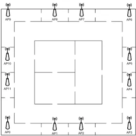
In the simulation, we consider a_{100 × 100 square meters sensing field. See} Figure Figure 4.1.

AP0

AP1 AP2 AP3

AP4 AP5 AP6 AP7 AP8 AP9 AP10 AP11

Figure 4.1: An illustration of the simulation environment.

(95, 60), (95, 95), (60, 95), (40, 95), (5, 95), (5, 60) and (5, 40). The solid lines in-dicate walls. The walls will not only affect the path loss of radio frequency signals but also limit the mobility of users. Particles will be filter out if their trajectories cross the walls.

4.1

Singal Path Loss Models

The signal path loss model we apply here is a variation of RIM [18]. LetPV SP

t (bj)

signal strength at locationl. Then,

Pr(ℓ, bj) = PtV SP(bj) − P LDOI(ℓ, bj) − P LOBS(ℓ, bj)

+ N(0, σf), (4.1)

whereP LDOI_{(ℓ, b}

j) is the path loss caused by obstacle, P LOBS(ℓ, bj) is the path

loss caused by the obstacles in the environment, andN(0, σf) representing

back-ground noises is a zero-mean normal distribution random variable with a standard deviationσf. Details are given below.

PV SP

t is hardware-dependent and also affected by the remaining battery level

that is modeled by a variance of sending power (VSP), e.g.,

PV SP

t = Pt× (1 + N(0, V SP )) , (4.2)

wherePtdenotes the initial transmit power andN(0, V SP ) is a zero-mean normal

distribution random variable with a standard deviationV SP . Each AP randomly initials itsPV SP

t as the simulation starts.

In real-world environments, the irregularity of signal fading is a common phe-nomenon. However, most path loss models do not take this non-isotropic property into consideration. In our simulation, the degree of irregularity (DOI) is applied to control the amount of path loss in different directions, e.g.,

P LDOI_{(ℓ, b}

j) = P L(kℓ, bjk) × Ki, (4.3)

co-efficient Ki is to reflect the level of irregularity at degree i = 0, · · · , 359 such that Ki =        1 ifi = 0 Ki−1± W (0, σd, γ) × DOI if i = 1..359 (4.4)

where_|K0− K359| ≤ DOI and W (0, σd, γ) is a zero-mean Weibull random

vari-able. The parameter DOI controls the allowable difference of two consecutive degrees1_{. Specifically, a larger |K}

i− 1| means that the amount of path loss has

greater deviation from the optimal path loss formulation at the i-th degree. The iterative definition ofKilets the variation of irregularity be continuous.

In an indoor environment, complicate partition is one of the major factors which influence the performance of positioning algorithms. When signals pene-trate through obstacles, such as walls, dramatic signal attenuation is companioned. The path lossP LOBS_{(ℓ, b}

j) stands for the amount of signal strengths absorbed by

obstacles between the transmitterbj and the receiver at ℓ. We adopt the concept

of wall attenuation factor (WAF) proposed in [2]:

P LOBS_{(ℓ, b}

j) = min(Nobs, maxW ) × W AF, (4.5)

where Nobs is the number of obstacles which exist in the middle of the

line-of-sight path of signal transmission from bj to ℓ, maxW is the maximum number

of obstacles that can influenceP LOBS_{(ℓ, b}

j), and W AF is a parameter which

de-1_{The irregularity of those non-integer degrees can be inferred by interpolating the values of}

notes the amount of signal attenuation caused by one obstacle. Note that different materials may have differentW AF values.

The default parameters of the simulation is as below. The path lose reference power is37.3, path lose exponent is 3.3 and path lose noise deviation σf = 3. The

number of access pointsAP s = 8. The training grain size grain size = 1. 100 training samples will be collected at each training location. The mobility speed is

1 (m/s) and positioning period is 1 second. Pt = 15 for all APs, V SP = 0.02,

DOI = 0.004, maxW = 4 and W AF = 3. Finally, the number of particles of particle filter is500. In the simulation, we only adjust the corresponding parame-ters and the rest parameparame-ters are set to default value.

4.2

The Impacts of System Parameters

The number of APs, denoted as AP s, somehow means the dimensions of signal patterns and affects the accuracy of pattern-matching localization. However, it also reflects deployment cost and training effort. Refer to Figure 4.2. We can see the errors decrease obviously as AP s increases. The accuracy of NNSS decreases dramatically if AP s became fewer. However, based on the mobility model,P F MM alleviates this problem and outperforms others.

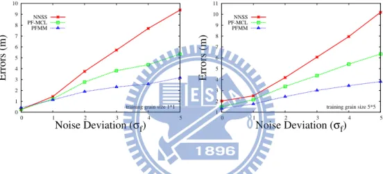
Noise disturbsRSSI received by users. That affects the accuracy of position-ing. We wonder if the noise problem can be mitigated by increasing the number

2 4 6 8 10 12 14 16 4 5 6 7 8 9 10 11 12 Errors (m) Access Points(APs) NNSS PF-MCL PFMM

Figure 4.2: An impact of theAP s.

0 1 2 3 4 5 6 7 8 9 10 0 1 2 3 4 5 Errors (m) Noise Deviation (σ_f)

training grain size 1*1

NNSS PF-MCL PFMM 1 2 3 4 5 6 7 8 9 10 11 0 1 2 3 4 5 Errors (m) Noise Deviation (σ_f)

training grain size 5*5

NNSS PF-MCL PFMM

Figure 4.3: An impact of noise deviation with training grain size.

of training locations. A small training grain size is used to increase the num-ber of training locations. Figure 4.3 illustrates the outcomes. The left figure is

with grain size = 1 and 10201 training locations, and the right figure is with

grain size = 5 and 441 training locations. The errors increase with the noise deviationσf. Nevertheless, the errors ofP F MM is within three meters no

0.05 0.1 0.15 0.2 0.25 0.3 0.35 0.4 0 0.005 0.01 0.015 0.02 Errors (m) DOI NNSS PF-MCL PFMM 2 2.5 3 3.5 4 4.5 5 5.5 6 0 0.005 0.01 0.015 0.02 Errors (m) DOI NNSS PF-MCL PFMM

Figure 4.4: An impact ofDOI.

1.5 2 2.5 3 3.5 4 4.5 5 5.5 6 0 0.5 1 1.5 2 2.5 3 3.5 4 Errors (m) WAF NNSS PF-MCL PFMM Figure 4.5: An impact ofW AF .

P F MM improves NNSS up to one half and P F MCL more than 25%.

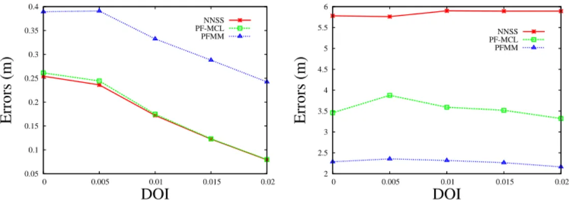
The DOI is used to reflect the irregularity of radio frequency signals. The

larger DOI is used, the more irregular the RSSI patterns become. We measure the errors with variousDOI setting in the environment with different noise devi-ationσf = 0 and σf = 3. In Figure 4.4, the left figure is for σf = 0 and the right

2 2.5 3 3.5 4 4.5 5 5.5 6 6.5 0 10 20 30 40 50 Errors (m)

Angle Dynamic (degree) NNSS Distance Dynamic 0% Distance Dynamic 10% Distance Dynamic 20% Distance Dynamic 30% Distance Dynamic 40%

Figure 4.6: An impact of estimating dynamic ofIMU Sensors.

The impact of signal noise is superior toDOI.

W AF is the wall attenuation factor representing the complexity of indoor en-vironments. LargeW AF implies that the RSS decreases dramatically when pass-ing wall. In Figure 4.5, we can see an apparent decreaspass-ing trend as the W AF increases.

At last, we evaluate the impact of performance by varying estimating dynamic of the sensors. In our localization engine, we refer to the RSSI patterns and sensor measurements for positioning. Hence, the measuring errors of sensors will be corrected by theRSSI patterns.

Now, we increase the measuring dynamic of sensors with signal noise (σf = 3)

as Figure 4.6 to evaluate the robust of P F MM. We set the mobility speed at 5 to strengthen the impact. As we can see, the system is robust. Besides, the other analysis is that the effects of angle dynamic is much bigger than distance dynamic.

Chapter 5

System Implementation

The system is divided into three parts to implement which are mobile user, posi-tioning server, and localization environment. The mobile user carries an Android smart phone, called HTC magic and equipped with a WiFi interface, and an IMU, called 3DM-GX1 made by MicroStrain company. The dimension of HTC magic

is _{113 mm × 55.56 mm × 13.65 mm, and its weight including battery is 118 g.}

The version of the android operating system is 1.5. It supports 2G (GSM), 2.5G (GPRS), 3G (WCDMA) and WiFi 802.11 b/g networks. And, the GPS, G-sensor and electronic compass are embedded. 3DM-GX1 is composed of one triaxial ac-celerometer, one triaxial magnetometer, and one triaxial angular rate gyroscope. The dimension of 3DM-GX1 is_{64 mm × 90 mm × 25 mm, and its weight is 75} grams. The IMU can provides 3D g-values in the range of _{±5 g, 3D magnetic} field in the range of_{±1.2 Gauss, and the rate of rotation in the range of 300}◦

second. The sampling rate of these readings is350 Hz at most. In addition, it can provide its orientation in Euler angle (pitch, roll, yaw) but at most in the rate of 100 Hz. The 3DM-GX1 communicates with the handheld device via an RS-232 or RS-485 interface. The optional communication speeds are19.2, 38.4 and 115.2 kBaud.

The 3DM-GX1 is equipped by user with the belt as Figure 2.1. We gain the prompt mobility and behaviors of user by it‘s measurements. For instance, we adopt a proposed walking judged algorithm using accelerations to simulate a pe-dometer. Therefore, it can determine that the user is walking or stopping, and cumulate the strides. And, we use the yaw of euler angle directly to simulate the electronic compass to track the orientations of user.

The g-sensor communicates with the mobile device via a UART interface or Zigbee protocol. The mobile device has the ability to sense Wi-Fi radio signals sent from surrounding access points. In the localization, the user are positioned accordance with the positioning interval. We use a program to collect the Wi-Fi radio signals and IMU sensor measurements regularly. And then, the sensor measurements will be imported into the Behavior Predicting Module. When po-sitioning interval expired, a popo-sitioning pattern including RSS, strides, heading, and user’s behaviors will be packaged and send to the positioning server via the WLAN. Secondly, once the positioning server receives a positioning pattern, the positioning pattern will be inputted to the positioning algorithm. Upon the

lo-calization result is estimated, it will be forwarded to the mobile user for demon-strating. In the last part, the environment of localization is a multi-storey building deploying WLAN infrastructure. The floor layout maps of the building are con-structed in 2.5-dimensional (2.5D) description including hallways, rooms, walls, stairways and elevators. In the localization, the positioning server uses it as the positioning reference.

The performances are evaluated by the errors of localization in the building

(the4th, 5th and 6th floors) of the Computer Science Department at the National

Chiao Tung University, Engineering Building III. The dimensions of the floors

are74.4 meters by 37.2 meters. The map of the positioning area is represented in

the 2.5D format to assume that the feet of the user are constrained to lie on the floor during the stance phase. It is consisted of the floor plane maps including walls and rooms. And, they are connected by the stairways and elevators. In the positioning, this map will be imported into the localization system. There are153 fingerprints deployed randomly on the hallways and other public areas of the map. Each of them is trained by 100 RSS patterns. The performances are contrasted with the nearest neighbor in signal space (NNSS), the mobility free particle filter (P F MCL) and our sensor enhanced particle filter (P F MM) by moving around in the positioning area. The number of particles of these particle filter approaches

is500. The user is positioned with the period per second, and the average amount

4.92 and 3.01 meters individually. The P F MM improves NNSS by 59% and P F MCL by 39%.

Chapter 6

Conclusions

In this paper, we developed an application level location tracking system. We proposed a sensor-enhanced particle filter scheme to assist the RF-based pattern matching localization system by user‘s immediate information. The user equips the IMU sensors (called G-Sensor) and electronic compass (called M-Sensor)with the belt. And, the sensor measurements will be converted to a mobility model. Based on these models, we enhanced the sampling stage of the traditional particle filter. The particles will be propagated by horizontal displacement vector and vertical displacement vector to close the user. And, we added a particle filtering module between the particle sampling module and particle weighting module. The incredible particles will be filtered out by speed filtering and passing wall filtering with maps information. We examined the performance by errors of localization in the simulation and experiment. According to the statistics in the simulation,

our performances are outstanding in spite of any environment. And, our engine is robust regardless the increasing of sensor errors. In the experiment, we improved NNSS by 59% and P F MCL by 39%.

Bibliography

[1] M. Addlesee, R. Curwen, S. Hodges, J. Newman, P. Steggles, A. Ward, and A. Hopper. Implementing a Sentient Computing System. Computer, 34(8):50–56, 2001.

[2] P. Bahl and V. N. Padmanabhan. RADAR: An In-building RF-based User Location and Tracking System. In IEEE INFOCOM, volume 2, pages 775– 784, 2000.

[3] S. Beauregard, Widyawan, and M. Klepal. Indoor pdr performance enhance-ment using minimal map information and particle filters. In Position, Lo-cation and Navigation Symposium, 2008 IEEE/ION, pages 141–147, May 2008.

[4] E. Brassart, C. Pegard, and M. Mouaddib. Localization using infrared bea-cons. Robotica, 18(2):153–161, 2000.

[5] B. Ferris, D. Hhnel, and D. Fox. Gaussian processes for signal strength-based location estimation. In In Proc. of Robotics Science and Systems, 2006.

[6] D. Fox, J. Hightower, L. Liao, D. Schulz, and G. Borriello. Bayesian Filter-ing for Location Estimation. IEEE Pervasive ComputFilter-ing, 2(3):24–33, 2003.

[7] S.-P. Kuo and Y.-C. Tseng. A Scrambling Method for Fingerprint Position-ing Based on Temporal Diversity and Spatial Dependency. IEEE Trans. on Knowledge and Data Engineering, 20(5):678–684, 2008.

[8] D. Niculescu and B. Nath. Ad Hoc Positioning System (APS) Using AOA. In IEEE INFOCOM, volume 3, pages 1734–1743, 2003.

[9] J. J. Pan, J. T. Kwok, Q. Yang, and Y. Chen. Multidimensional Vector Regression for Accurate and Low-Cost Location Estimation in Pervasive Computing. IEEE Trans. on Knowledge and Data Engineering, 18(9):1181– 1193, 2006.

[10] N. B. Priyantha, A. Chakraborty, and H. Balakrishnan. The Cricket Location-Support System. In ACM/IEEE MOBICOM, pages 32–43, 2000.

[11] A. Savvides, C.-C. Han, and M. B. Strivastava. Dynamic Fine-Grained Lo-calization in Ad-Hoc Networks of Sensors. In ACM/IEEE MOBICOM, pages 166–179, 2001.

[12] S. Thrun, D. Fox, and W. Burgard. Monte carlo localization with mixture proposal distribution. In Proc. of the National Conference on Artificial In-telligence, 2000.

[13] T.-C. Tsai, C.-L. Li, and T.-M. Lin. Reducing Calibration Effort for WLAN Location and Tracking System using Segment Technique. In IEEE Int’l Conf. on Sensor Networks, Ubiquitous, and Trustworthy Computing (SUTC), volume 2, pages 46–51, 2006.

[14] Widyawan, M. Klepal, and S. Beauregard. A novel backtracking particle filter for pattern matching indoor localization. In MELT ’08: Proceed-ings of the first ACM international workshop on Mobile entity localization and tracking in GPS-less environments, pages 79–84, New York, NY, USA, 2008. ACM.

[15] O. Woodman and R. Harle. Pedestrian localisation for indoor environments. In UbiComp ’08: Proceedings of the 10th international conference on Ubiq-uitous computing, pages 114–123, New York, NY, USA, 2008. ACM.

[16] L.-W. Yeh, M.-S. Hsu, Y.-F. Lee, and Y.-C. Tseng. Indoor localization: Au-tomatically constructing today’s radio map by irobot and rfids. In IEEE Sensors Conference, 2009.

[17] J. Yin, Q. Yang, and L. M. Ni. Learning adaptive temporal radio maps for signal-strength-based location estimation. IEEE Transactions on Mobile Computing, 7(7):869–883, 2008.

[18] G. Zhou, T. He, S. Krishnamurthy, and J. A. Stankovic. Impact of Radio Irregularity on Wireless Sensor Networks. In ACM MobiSys, pages 125– 138. ACM Press New York, NY, USA, 2004.