結合獨立成份與色彩特徵之平均移動向量人形 追蹤演算法-應用於主動式攝影機

國 立 交 通 大 學

電控工程研究所

碩 士 論 文

結合獨立成份與色彩特徵之平均移動向量人形

追蹤演算法-應用於主動式攝影機

Mean-shift human tracking based on combination

of ICA and color feature on active camera.

研 究 生：劉哲男

指導教授：林進燈 博士

中華民國 九十九 年 七 月

結合獨立成份與色彩特徵之平均移動向量人形追蹤演算法

-應用於主動式攝影機

Mean-shift human tracking based on combination of ICA and

color feature on active camera.

研 究 生：劉哲男 Student：Che-Nan Liu

指導教授：林進燈 博士

Advisor：Dr. Chin-Teng Lin

國立交通大學

電控工程研究所

碩士論文

A Thesis

Submitted to Institute of Electrical Control Engineering

College of Engineering and Computer Science

National Chiao Tung University

in Partial Fulfillment of the Requirements

for the Degree of Master

in

Electrical and Control Engineering

June 2010

Hsinchu, Taiwan, Republic of China

結合獨立成份與色彩特徵之平均移動向量人形

追蹤演算法-應用於主動式攝影機

學生：劉哲男

指導教授：林進燈 博士

國立交通大學電控工程研究所

摘要

近幾年來，基於視覺的偵測和追蹤在電腦視覺領域上是一項很重要的課題， 基於視覺的監控系統已經被廣泛的應用在停車，病人監控以及安全監控...等領域 上。在本論文當中實現了在主動式攝影機上完成人物偵測和追蹤，在過去主動式 攝影機追蹤是利用影像相減的方式找出移動物體的位置，透過移動物體的位置來 驅動攝影機的雲台，雖然這樣的方法可以對移動物體作追蹤但是為了要找到移動 物體的位置攝影機在移動的過程中必須停下來才可以做影像相減，所以會造成攝 影機無法連續的控制雲台，換句話說，假如雲台持續的轉動，因攝影機的轉動會 得到模糊的影像而且相減時不僅會得到移動物體也會得到包含背景的資訊。針對 利用相減的方法無法找到移動物體精確的位置，因此我們提出結合獨立成份與色 彩特徵之平均移動向量人形追蹤演算法應用於主動式攝影機來解決上述的問題。 本論文主要分成三大部分，分別是人物偵測、追蹤和攝影機的控制。利用人 物偵測系統獨立成分分析和支持向量機(Support Vector Machines)分類現在畫面 中的移動物體是人還是非人。當我們系統偵測到人之後就會被鎖定，利用平均移 動向量演算法在每一張輸入的影像計算出相似度並且送出控制命令給主動式攝 影機，使畫面中的人可以保持在我們所監控的影像中。有時候人會整個或部分的 被其他物體遮蔽，因此相似度會劇烈的下降，使平均移動向量在追蹤的時候無法

追蹤目標物，為了解決遮蔽的情況我們採用卡爾曼濾波器對目標物做位置的預 測。 當目標物和背景有相同顏色的情況下只使用顏色當作平均移動向量追蹤特 徵會有遺失的現象。為了解決遺失的現象，我們提出一個結合獨立成分分析和顏 色當特徵的先進平均移動向量演算。因為獨立成分模組在訓練時所輸入的灰階影 像具有人物的特性，因此我們提出來的驗算法可以有效在相同顏色下判斷人或背 景。

Mean-shift human tracking based on combination

of ICA and color feature on active camera

Student: Che-Nan Liu

Advisor: Dr. Chin-Teng Lin

Institute of Electrical Control Engineering

National Chiao Tung University

Abstract

In recent years, detection and tracking are important tasks in computer vision for visual-based surveillance system. Visual-based surveillance system is a widespread application in parking, patient monitoring and security surveillance fields. In this thesis, we use human detection and tracking algorithm based on active camera. In the past, active camera based object tracking used temporal difference to find object position and then drive pan or tilt command to control the active camera. Although this process can achieve moving object tracking. However, to find moving object position, the active camera should be stopped for the computation of temporal difference. Therefore, the active camera can not pan/tilt continuously and smoothly. In the other words, if the active camera is able to keep moving the whole time, we will capture blur images, and temporal difference will extract not only moving object but also background. Therefore, it is impossible to accurately locate the position of moving object by using temporal difference while the active camera is moving. So we propose mean-shift human tracking based on combination of ICA and color feature on active camera to solve above problem.

pan/tilt control. In human detection system, the independent component analysis (ICA) and support machine vector (SVM) classifier are applied to classify moving objects into human or non-human. When a human is detected then we need to track it. Mean-shift algorithm will track the target by computing the similarity value in every frame and send the position to active camera, and then active camera will drive PTZ to keep the target in the center of FOV (field of view). Sometimes human will be partially or fully occluded by other object, thus the similarity will drastically decrease. Consequently, mean-shift will miss the target. To overcome the above problem, the Kalman filter is applied to predict the target’s position in next frame.

The mean-shift using only color feature will miss the tracking target, when the target object and background have the same color. In order to solve the missing problem, we propose a novel mean-shift algorithm based on combination of ICA and color feature. Since the ICAs modeled human characteristic with gray-level training data, the proposed algorithm can distinguish human and background with the same color.

Chinese Acknowledgements

致 謝

兩年的碩士班生活即將告一段落，能夠在此經過各位老師的指點是我此生的 榮幸，尤其是我的指導教授林進燈博士，這兩年來的細心指導與督促，讓我學習 到許多寶貴的知識與經驗，在學業及研究方法上也受益良多。另外也要感謝口試 委員陶金旺教授以及許騰尹教授在口試時的指點與鼓勵，使得本論文更為完整。 其次感謝超視覺影像實驗室的大家長鶴章、剛維學長的指導，以及博士班的 學長姐肇廷、Linda 以及東霖給予我指導與建議，尤其是 Linda 學姊給予我許多 建議與方向，在生產前一天還是持續給予指導與論文上的指點，直到最後一刻才 放鬆心情生產，本論文多虧學姊的幫忙。也感謝同學佳芳、聖傑、嶸健及健豪的 相互砥礪，還有實驗室的學弟妹郁光、開澄、奎理、庭立、奕竹、慶峰及皕文， 在生活上給予諸多的協助，讓我在這兩年的研究生涯，無論是課業上、學業上或 是生活上都不孤單。 最後，更要感謝我的父母，從小到大的教育及栽培，讓我有勇氣去追求我想 要的，讓我無後顧之憂，如果沒有他們無怨無悔的付出，沒有他們就沒有今日的 我。 謹以本論文獻給我的家人及所有關心我的師長與朋友們。

Contents

Chinese Acknowledgements ... vi  Contents ... vii  List of Tables ... ix  List of Figures ... x  Chapter 1 Introduction ... 1  1.1 Motivation ... 2  1.2 Related Work ... 3 

Chapter 2 System Overview ... 7 

2.1 Active camera control ... 7 

2.2 Software system ... 9 

Chapter 3 Object extraction and Human detection ... 11 

3.1 Moving object extraction ... 11 

3.2 Human detection ... 14 

3.2.1 ICA feature extraction ... 15 

3.2.2 Entropy feature selection ... 16 

3.2.3 SVM classifier ... 18 

Chapter 4   Human tracking ... 20 

4.1 features ... 21  4.1.1 color feature ... 21  4.1.2 ICA feature ... 23  4.2 Kernel functions ... 24  4.3 Mean-shift algorithm ... 25  4.4 ROI resize ... 30  4.5 Kalman filter ... 34 

Chapter 5   Experimental results ... 42 

5.1 Environment setup ... 42 

5.2 Kalman filter ... 44 

5.3 Active camera with single object experiment ... 47

5.3.1 9 regions and 26 regions experiments……….47

5.3.2 Color spaces experiments………50

5.4 Human tracking in multiple objects experiment……….59

Chap 6 Conclusions and Future work ... 63 

6.1 Conclusions ... 63 

6.2 Future works ... 63 

List of Tables

Table 4-1 MAE in different frame motion………...39

Table 4-2 MAE in different frame motion...41

Table 5-1 Predicted position...44

List of Figures

Fig. 1-1 Three categories of tracking……….3

Fig.2-1 Active camera control through RS-485……….7

Fig.2-2 message format………..8

Fig2-3 Data byte 1 to 4 format………...…8

Fig.2-4 Divide screen into 25 regions………9

Fig.2-5 Control direction for each regions……….9

Fig.2-6 system overview……….. ………...10

Fig. 3-1 Human detection system………...…..11

Fig. 3-2 Moving object extraction………....13

Fig. 3-3 Moving object extract processing………...14

Fig. 3-4 Human detection flow chart………...…….15

Fig. 3-5 Image decomposition……….………15

Fig. 3-6 Optimal separating hyperplane……….. 19

Fig. 3-7 Analysis of feature selection………...………19

Fig. 4-1 Human tracking flow chart………...…..20

Fig.4-2 (a) RGB color model (b)HSV color model. ………....22

Fig. 4-3 (a) Human’s ROI (b) Kernel function (c) Histogram of color feature………23

Fig. 4-4 Color and ICA feature histogram………....24

Fig. 4-5 (a) Gaussian kernel (b) flat kernel (c) Epanechnikov kernel………..…25

Fig. 4-6 (a) Target object (b) Kernel function (c) Target object and Kernel function..25

Fig. 4-7 Mean-shift algorithm flow chart……….…29

Fig. 4-8 ROI scale larger than object………...30

Fig. 4-9 ROI resize flow chart……….31

Fig. 4-10 X-axis and Y-axis image projection………..32

Fig. 4-11 Fixed camera condition………32

Fig. 4-12 Active camera condition………...34

Fig. 4-13 Kalman filter flow chart………...34

Fig. 4-14 Indoor environment………..38

Fig. 4-15 (a) previous 2 frame motion left is x and right y position (b) previous 5 frame motion left is x and right y position………...39

Fig. 4-16 Outdoor environment………..…..40

Fig. 4-17 (a) previous 2 frame motion left is x and right y position (b) previous 5 frame motion left is x and right y position………...41

Fig. 5-1 Experimental environment……….………43

Fig. 5-2 Experiment zoom condition………43

Fig. 5-4 Human tracking use mean-shift and Kalman filter……….47

Fig. 5-5 9 regions pan/tilt control….. ………..48

Fig. 5-6 Position based use 9 regions………...………49

Fig. 5-7 Position based use 25 regions……….50

Fig. 5-8 Choice RGB color space……….51

Fig. 5-9 Choice Y’VU color space. ……….52

Fig. 5-10 Sample of chair………..………...54

Fig. 5-11 Sample of chir3……….54

Fig. 5-12 Sample of chair2………...54

Fig. 5-13 Sample of chair2………...54

Fig. 5-14 Using color feature………...56

Fig. 5-15 Using color and ICA features……….…..57

Fig. 5-16 Zoom in/out tracking………....59

Fig. 5-17 Across case….. ………61

1

Chapter 1

Introduction

In recent years, detection and tracking are important task in computer vision for visual-based surveillance system. Visual-based surveillance system has widespread application in parking, patient monitoring and security surveillance fields, etc. In visual-based surveillance, human eyes are used to watch surveillance in front of monitor in the past years. Although using human eyes to watch surveillance system works well, but it still has some problems. For example, finding human resource to watch monitor all day long is expensive and it can not achieve real-time surveillance. In order to achieve real-time and all day long surveillance, automatic visual surveillance in computer vision plays an important role in security area.

Human detection and tracking surveillance are important topics in computer vision and security area. The human detection system consists of two parts: moving object extraction and human classification. The moving object extraction to extracting objects from background and locate its position and size. Meanwhile, the human classification is classifying the moving object into human or other objects. After human detection, the human tracking system will trace the target object all the time. Sometimes, target human would be occluded with other object while tracking, thus tracking system which has prediction ability is needed in this case.

There are two kinds of camera used in security surveillance, fixed and active camera. The fixed camera is very popular and low cost, but it’s FOV (filed of view) limited. If human is walking out of monitoring area, tracking system can not keep monitoring. In order to keep target human in the camera scene, active camera is the best choice because it has the ability to perform pan, tilt and zoom in/out

automatically. In this thesis, we integrate the real-time human detection, human tracking and kalman filter to achieve an active camera-based visual surveillance system.

1.1 Motivation

2 In this thesis, we present a human tracking system on active camera. We concern on the active camera because the ability of active camera to drive pan-tilt-zoom (PTZ) to keep the target human in the monitoring area (FOV). Mostly, tracking system on active camera only track a moving objects even the moving object is not human being. Therefore, it motivates us to research a system which used active camera and has the ability to track only target human. We proposed a human detection system using ICA (independent component analysis) base on conditional entropy for feature extraction and SVM (support vector machine) to classify human or other objects.

3

Generally, tracking system on active camera is using temporal difference to extract moving object from background. It will cause the active camera unable to continuously and smoothly drive PTZ. In the other words, if the camera still drive PTZ, we will capture blur images and temporal difference will extract not only moving object but also object that have edge includes background. Therefore, it will impossible accurately to locate the position of moving object. We applied mean-shift tracking algorithm to solve this problem. The mean-shift algorithm will locate the maxima of a density function given histogram feature through iteration and it works frame by frame. The histogram feature is combination of color and ICA features. The color feature will keep the human color information for example clothes, meanwhile ICA feature will keep the feature of human being.

When target human partially or fully occluded with other object, we will use Kalman filter to predict the position in the next frame.

4

1.2 Related Work

Fig. 1-1 Three categories of tracking

In recent years, many human detection systems are developed. The human detection system determines the object position and size in the image. A good human detection system can provide valuable insight on how one might approach other similar feature and pattern detection system. There are two parts of human detection system, segmentation of moving object from background and discrimination of humans from nonhuman objects. A moving object occurred in the image will be extracted from background image in the human detection system. There are many human detection method are used to detect the human that presence in an image. Optical flow is used to estimate independently moving object, but it expense complex computation and sensitive to change of intensity. Optical flow is used in [2,6] to detect vehicle. Zhao et al [8] exploited stereo based segmentation algorithm to extract object from background and to recognize the object by neural network based recognition. Although stereo vision based technique have been proved to be more robust it require at least two cameras and can be used only for short and middle

distance detection. Dalal and Triggs [7] use gray scale image to get edge image and using it to extract orientated gradient. They select the dominant orientated gradients to detect human. In [8] a stereo-based segmentation algorithm is used to extract objects from the background, followed by a neural network-based recognition. Sebastian and Alvaro [10] present a new computer vision algorithm designed to operate with moving cameras and to detect humans in different poses under partial or complete view of the human body. Boosting detector cascades have been introduced by Viola et

al. [13]. In this, AdaBoost is used in each layer to iteratively construct a strong

classifier guided by user-specified performance criteria. Viola et al. contribute to the high processing speed of the cascade approach, since usually only a few feature evaluations in the early cascade layers are necessary to quickly reject non-pedestrian examples. In [14] presents a template-based approach to detecting human silhouettes in a specific walking pose, templates consist of short sequences of 2D silhouettes obtained from motion capture data.

Human tracking system is used to follow target human through the sequence images in terms of changes in scale and position. As mentioned in introduction, there are two type of real-time tracking system. One is tracking object with fixed camera and the other is with an active camera. Tracking object with an active camera can keep the object in the scene of camera by drive pan and tilt. The active camera also have zoom in/out function that can used to zoom in/out object when the object’s image resolution is too small to track. The active camera used in surveillance system needs to achieve real-time tracking. If an tracking algorithm expense more computation time then the active camera will not track object immediately. Many tracking system are used active camera work only on pan-tilt or zoom. The objective of our approach is to correctly select the target human, and drive pan/tilt to keep target

maximum size the zoom function will operate zoom-in or zoom-out. There are many application of active camera. Murray et al. [30] utilized morphological filtering of motion images for background compensation. This motion tracking method can track a moving object from dynamic images with pan/tilt angles. C. Lin et al. [31] use an image mosaic technique to track moving objects with a single pan/tilt camera indoors. Collins et al. [32] developed a system with multiple cameras that tracked a moving figure using pan/tilt cameras alone. This system used a kernel-based tracking approach to overcome the apparent motion of the background as the camera moved. L. Fiore et al. [33] use wide angle and active camera to achieve human tracking. In this work the target object was found by wide angle camera and through camera calibration method tell active camera the pan/tilt angle to track the object.

In Fig. 1-1, there are three kinds of tracking method. Feature based is the most commonly method. Color, edge or motion are commonly used as tracking feature. The edge detection methods, such as Sobel method [3], Laplacian method [3], and Marr–Hildreth method [4] etc., utilize masks to do convolution on the image to detect the edges based on the abrupt change of the gray level. Wei Guo et al. [1] proposed human tracking system based on shape analysis. Law et al. [5] design fuzzy rules use in edge based human tracking, although this method requires a rather large and complicated rules set. However, these methods are need more computation time and edge pixels can not be always detected continuously. We noted that all those methods mentioned above detect edges using gray level images, and those methods will be neglect for color images because the representation of a pixel is not only a gray level but a vector in a color space. The edge occurring in the adjacent pixels which have the same values in any one color component may not be detected. So edge detection only in gray level image is not sufficient and robust. Pattern recognition learning the target object to search them in sequence image can achieve human tracking. Williams et al.

[26] extended the approach to the nonlinear translation predictors learned by Relevance Vector Machine. Agarwal and Triggs [27] used RVM to learn the linear and nonlinear mapping for tracking of 3D human poses from silhouettes. Bohyung Han and Larry Davis [28] use PCA to extract feature from color and use these feature in mean-shift algorithm to implement object tracking. Robert T. et al. [29] presents an online feature selection mechanism for evaluating multiple features while tracking and adjusting the set of features used to improve tracking performance. Their feature evaluation mechanism is embedded in a mean-shift tracking system adaptively selects features for tracking. The mean-shift algorithm was originally proposed by Fukunaga and Hosterler [9] for clustering data. The kernel-based object tracking proposed by Meer et al [19]. This method tracks an object region represented by a spatial weighted intensity histogram. So the target and candidate object distinguish whether they are similar by Bhattacharyya coefficient, and tracking is achieve by optimizing this objective function using the iterative mean-shift algorithm. Later, many variants of the mean-shift algorithm were proposed for various applications [20-23].

Though the mean-shift object tracking algorithm performs well on sequences with relatively small object displacement, its performance is not guaranteed when objects undergo partial or full occlusion. In order to improve the performance of mean-shift tracker, in the event of object undergoing partial occlusion, there some method was be proposed Kalman filter [34,35] and particle filter [24,25]. K. Nummiaro et al [25] use the idea of particle filter to apply a recursive Bayesian filter based on sample sets. They use color as feature. Their work have evolved from the condensation algorithm which was developed in the computer vision community.

Plamen P. et al [15] use the mean-shift method for face detection and automated control of an active camera to follow a person’s face and keep his image centered in

5

Chapter 2

System Overview

2.1 Active camera control

6

7 Fig.2-1 Active camera control through RS-485

8 The proposed system is using active camera to track and keep human in the center of monitor screen or camera’s FOV (field of view). The active camera is controlled by pelco P-protocol [16] through RS-232 to RS-485 converter. We have to control pan (left, right direction), tilt (up, down direction) angle, and zoom’s step to achieve our tracking purpose.

9 The pelco P-protocol has 8 bytes data with message format as show in Fig. 2-2. Byte1 and byte7 are start and stop byte, and always set to 0xA0 and 0xAF, respectively. Byte2 is the receiver or camera address. In our case, we only use one camera therefore byte2 always sets to 0x01. Byte3-6 are use to control pan-tilt-zoom ( PTZ) as shown in Fig. 2-3. The last byte is an XOR check sum byte.

11

Fig.2-2 message format

12

Bit 7 Bit 6 Bit 5 Bit 4 Bit 3 Bit 2 Bit 1 Bit 0

Data byte1 Fixed to 0 Camera on Auto scan on

Camera

On/Off Iris close Iris open Focus near Focus far Data byte2 Fixed to 0 Zoom wide Zoom tele Tilt down Tilt up Pan left Pan right 0 (For

pan/tilt) Data byte3 Pan speed $00 (stop) to $3F (high speed) and %40 for Turbo

Data byte4 Tilt speed $00 (stop) to $3F (high speed)

13

14 Fig2-3 Data byte 1 to 4 format

15

16 In this thesis, we divide the image view into 25 regions to drive PTZ and keep moving object in the center of FOV. Every region has specific direction, angle and speed as shown in Fig. 2-5. If the target is located on stop-region, then camera will set to stop. Otherwise, if the target is located on other regions. For example in the region H the camera will drive to up direction, so on. The zoom-in and zoom-out will be activated if the target’s size become smaller or larger than user’s define size. For example, if the target’s size 1.5 times larger than user’s define size then the zoom-out will activated. Otherwise, if the target’s size is 0.5 times smaller than user’s define size, then zoom-in will activated. During the period of the active camera moving, the tracking system is still running as well as the camera control system. So, if the moving object changes its direction, we can easily change the control action immediately.

17

A

B

C

D

E

F

G

H

I

J

K

L

Stop

M

N

O

P

Q

R

S

T

U

V

W

X

18 Fig.2-4 Divide screen into 25 regions

19

20

21 Fig.2-5 Control direction for each regions

2.2 Software system

22 The whole system consists of three major parts: Human detection, human tracking and PTZ control. Input frame are captured by active camera with resolution 320x240 and moving object will be extracted by background difference. We use previous 20 frames to build a background image. The independent component analysis (ICA) and support machine vector (SVM) classifier are applied to classify the moving object into human or non-human. When a human is detected then we need to focus on it. Mean-shift algorithm will

track the target by compute the similarity value in every frames and send the position to active camera, then active camera will drive PTZ to keep the target in the center of FOV. Sometimes human will be partially or fully occluded by other object, thus the similarity will drastically decrease, consequently mean-shift will miss track the target. In this case, the Kalman filter is activated to predict the target’s position in next frame.

23 PTZ camera Zoom in & out control Moving object extraction Human detection Mean-shift human tracking Kalman Filter: position Predict

Image source part Human detection part Human tracking part PTZ control part

Pan & Tilt control

Occlusion??

Static Dynamic

Chapter 3

Object extraction and Human detection

24

25

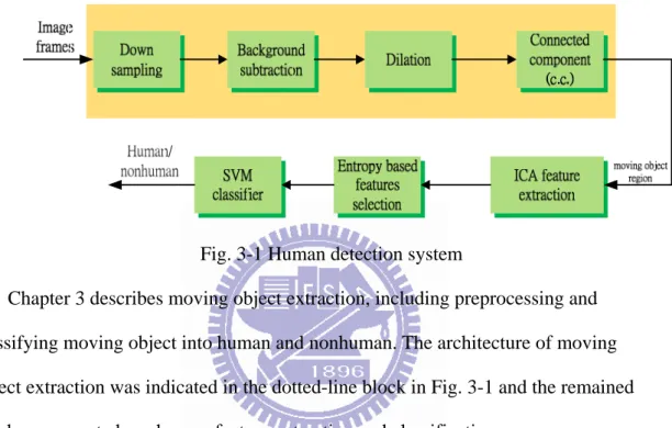
Fig. 3-1 Human detection system

Chapter 3 describes moving object extraction, including preprocessing and classifying moving object into human and nonhuman. The architecture of moving object extraction was indicated in the dotted-line block in Fig. 3-1 and the remained blocks represented our human feature extraction and classification.

3.1 Moving object extraction

26 Mostly, in surveillance system, the default position of camera is fixed even the camera is an active camera, so we can use the still image as background image. Background subtraction is the simplest way to extract moving object from an image. Besides, we used the background subtraction method in order to meet the real-time requirement.

27 Our background image was constructed by using first 20 frames. The difference for each pixel (x, y) could be calculated by

28 IBS( , ) |x y = IC( , )x y −IB( , ) |x y (3.1)

29 where I_C and I_B denote the current and background gray image, respectively. BS

I denotes the background subtraction image. A threshold value ths is choose to oving object

produce binary m M_objas described in following equation.

30 (3.2)

31 The dilation process applied on

1 ( , ) ( , ) 0 ( , ) BS obj BS if I x y ths M x y id I x y ths ≥ ⎧ = ⎨ _< ⎩ obj

M to gradually enlarge the boundaries of moving object pixels (foreground). Thus areas of foreground pixels grow in size while holes within those regions become smaller.

32 i j (3.3) 33 (3.4) 34 1 1 1 1 ( , ) foreground obj i j T M =− =− =

∑ ∑

1 1 ( , ) 0 foreground D if T I i j otherwise > ⎧ = ⎨ ⎩ foreground

T in Eq. 3.3 denotes the total foreground pixel in a (3x3) dilation mask. If at least one pixel coincides with foreground pixel, then the center of (3x3) mask is sets to the foreground value. If all the corresponding pixels are background then it will set to background value.

35 Connectivity between pixels is a fundamental concept that simplifies the definition of numerous digital image concepts, such as regions and boundaries. To establish whether these two pixels are connected, it is determined by their neighbors and finds their gray levels satisfy a specified criterion or similarity. For instance, in binary image with values 0 and 1, two pixels maybe 4-neighbors, but they are said to be connected only if they have the same value. Connected component works by scanning an image, pixel-by-pixel in order to identify connected pixel regions and labeling the pixel that connected together with same

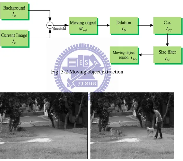
label. Once all groups have been determined, each pixel is labeled with a gray level or a color according to the component it was assigned to as shown in Fig. 3-2. After connected component, we observe the exist labels. In actual situation not all of them are belong to moving object pixels, therefore we use a (9x9) size filter to eliminate noise labels. The connected component without noise clearly observed in Fig. 3-2. All of these moving object extract result are show in Fig. 3-3. 36 B I C I obj M I_D I_CC SF I ROI I

Fig. 3-2 Moving object extraction

37

38

(b)

(c)

40 Fig. 3-3 Moving object extract processing. (a) Left is I_B. Right is I_C. (b) left is obj

M . Right is I_CC. (c) Left is I_SF. Right is I_ROI.

3.2 Human detection

We applied independent component analysis (ICA) on the foreground regions for feature extraction proposed. Then classified it into human or nonhuman by SVM classifier shown in Fig. 3-4.

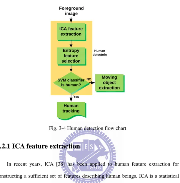
ICA feature extraction Foreground image Human tracking SVM classifier is human? Moving object extraction NO Yes Entropy feature selection Human detectoin

Fig. 3-4 Human detection flow chart

3.2.1 ICA feature extraction

In recent years, ICA [38] has been applied to human feature extraction for constructing a sufficient set of features describing human beings. ICA is a statistical method for transforming an observed multidimensional random vector into components that are statistically independent. ICA is a generalization of principle component analysis (PCA), it is a high-order statistic approach. As Fig. 3-5 shows ICA transforms each input image to the combination of bases and its corresponding coefficients.

1

u

×

u

₂

×

K

u

_n

×

Fig. 3-5 Image decomposition.

Let us have training images which include both human and non-human with images size are ( ). Reshape each image into a N-vector, then, the mixture data

m

×

r c

X is an (m x n) matrix.

Also the mixture data x x₁, ₂,...,x_m are the linear combination of n independent

and zero-mean of the source signal s s₁, ₂,...,sn (typically m ≥n) as described in 1 1 2 2 ...

x_j =h s_j +h s_j + +h s_{jn n} (3.5) The matrix H is expressed in terms of the elements h , and it is an unknown full _ji

m x N) mixture matrix. Since all vectors are column vectors and the transpose of

is a row vector, we can rewrite Eq. 3.5 to Eq. 3.6 by using vector-matrix notations

=HS (3.6)

ithout loss of generality, we assume that both the mixture variables and independent ponents have zero mean and non-Gaussian distributions. For the nonzero mean distributions, the observable variables

rank ( X X W com j x ean dis U fo

can always be centered by subtracting the ple mean to become the zero m tribution. If W denotes the inverse of the basis matrix S, the coefficients matrix r training matrix

sam

T

X will be expressed in

(3.7)

n-component base vectors which have the best distinguish ability for detecting

ans and nonhumans should be chosen from many candidate components.

3.2.2 Entropy feature selection

Unlike PCA features, the ICA features are not sorted, thus the conditional entropy is applied to feature selection, the sorting process and choosing an appropriate subset of ICA features. Sorting variables may be an important step to enhance the high-dimensional dataset, which gave us the idea to place correlated or similar

ensions close to each other in high-dimensional value space to help human user T

U =WX

The hum

If the entropy is the amount of information provided by a random variable, then our conditional entropy can be defined as the amount of information about one random variable provided another random variable. The entropy of a random variable reflects the more truthful information of the observed variable. If the variable is more random, it means unpredictable, which may result in the large entropy value.

The 2-D data space obtained from ICA feature extraction needs to be discretized into a matrix of a grid cell by separating each dimension into a set of intervals or bins. The discretization process begins with calculating the mean value of data in one dimension and dividing the data into two halves with that mean value. Recursively, each half is divided into halves with its own mean value. The recursion will stop when we obtain the required number of intervals or meet the constraint of total bins. Let a discrete random variable Z be with proposed values { ,z z_{1 2},...,z_m}. The information entropy of Z with the probability density p(z) is defined in

(3.8)

The conditional entropy quantifies the uncertainty of a random variable Y if given that the value of a second random variable Z is known. Each coefficient has to be normalized to [-1, 1] and quantized to n bins. Let Y= {-1, 1} be the desired class, the n the conditional entropy can be described in

(3.9) The conditional entropy (Y | Z) is a weighted sum of the entropy values in all columns, where the joint entropy is defined by

(3.10) We sort the conditional entropy (Y | Z) and use the sorted results to select corresponding independent components. The coefficients or independent components with the better classification ability are associated with the small conditional entropy.

1 ( ) ( ) log ( ) n i i i H Z p z p z = = −

∑

( | ) ( , ) log ( | ) ( , ) ( ) z y H Y Z = −

∑∑

p y z p y z =H Y Z −H Z ( , ) ( , ) log ( , ) z y H Z Y = −

∑∑

p z y p z y

The selected ICA features will be used in the SVM classifier to identify humans to nonhumans. The training database consisted of 1843 human and 840 nonhuman images with image size (40x40) pixels. The maximum number if ICA to 76 and we choose 30 best bases for SVM classifier.

3.2.3 SVM classifier

Support Vector Machines (SVMS) are developed to solve the classification and regression problem. SVM is a way which starts with a linear separable problem. For classification, the goal of SVM is to separate two classes by a function which is induced available example. Consider the example in Fig. 3-6, there are two classes of data and many possible linear classifier that can separate these data, but only one of them is the best classifier which can maximize the distance between two class-margin, this linear classifier is called optimal separate hyperplane. Fig. 3-7 shows the accuracy rate and the number of SV (support vector) foe all number of ICA to be 76. Based on this experiment result, the accuracy rate of human detection system will increase if number of IC is increasing. But in practice, we select 30 ICs because number of SVs is almost close to minimum and the accuracy rate more than 90%. The main reason to choose minimum number of SVs is to decrease the computation cost, in order to meet the real-time requirement.

Fig. 3-6 Optimal separating hyperplane

(a)

(b)

Chapter 4

Human

tracking

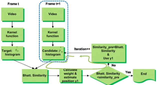
MS similarity Use predicted position Use original position Similarity <0.7 ? NO YES

Fig. 4-1 Human tracking flow chart

A human tracking system based on mean-shift algorithm is proposed in this thesis. The mean-shift algorithm is a simple iterative procedure that shifts each data point in its neighborhood and locating the maxima of a density function given discrete data sampled from that function [36]. Generally, the mean-shift algorithm uses color feature but in our thesis, we combine color feature and ICs (Independent Components analysis) feature. The idea behind the combination is come from human detection based on ICs feature in chap3. Although color feature able to track moving object but the combination color and ICs able to track not only moving object but moving human.

The Kalman filter is applied to predict the location of moving human in next frame. The Kalman filter actives when moving human partially occluded with other object, in other hand the mean-shift similarity value decrease until smaller than a

4.1 features

4.1.1 color feature

Most kernel based object tracking use color as feature. Color information extends into three dimensions of original grey scale image so it will increase good tracking performance. Most papers use mean-shift as tracking algorithm usually consider color as feature to accomplish object lock. We compare the performance of three color space: RGB, HSV and Y’UV. Based on experiment, the HSV color space give a good performance while tracking, thus we apply it on tracking with active camera.

HSV color transformation:

The main purpose of HSV color space transformation is to reduce the sensitivity of illumination or lightness information in RGB color space. In Fig. 3-6, Fig. 3-7 are RGB and HSV color space, respectively.

The HSV model, also known as HSB model, was created in 1978 by Alvy Ray Smith. It is a nonlinear transformation of the RGB color space. It defines a color space in terms of three components: hue, saturation, and value. The definition is described below: [16]

1. Hue: It is the color type and ranges from 0 ~ 360 degree. Each value corresponds to one color. For example, 0 is red, 45 is orange and 55 yellow. When it comes to 360 degree, it is also equal to 0 degree.

2. Saturation: It is the intensity of the color, and ranges from 0%~100%. 0 means no color, and that means only gray value between black and white exists. 100 means the intense color with the most color variety.

always black. Depending on the saturation, 100 may be white or a more or less saturated color.

(a) (b)

Fig.4-2 (a) RGB color model [17] (b)HSV color model [18]

The transformation algorithm from RGB color model to HSV color model could be described in the following equation.

0 60 0 , 60 360 , 60 120 60 240 if MAX MIN G B if MAX R G B MAX MIN G B if MAX R G B H _{MAX MIN} B R if MAX G MAX MIN R G if MAX B MAX MIN = ⎧ ⎪ ₋ ⎪ × + = − ⎪ ⎪ ₋ ⎪ × + = = ⎨ − ⎪ ₋ ⎪ × + = − ⎪ ⎪ ₋ × + = ⎪ − ⎩ ≥ < (4.1) 0 0 1 if MAX S _MIN Otherwise MAX = ⎧ ⎪ = ⎨ ₋ ⎪⎩ (4.2) (4.3) where MAX, MIN are maximum and minimum value of (R, G, B), respectively.

Y’UV color transformation

The Y’UV color model defines a color space in terms of one luma (Y') and two chrominance (UV) components. The Y'UV color model is used in the NTSC, PAL, and SECAM composite color video standards. Y' stands for the brightness component and U and V are the chrominance components. The transform equation are show

following: ' 0.299 0.587 0.114 0.14713 0.28886 0.436 0.615 0.51499 0.10001 Y R U V B ⎡ ⎤ ⎡ ⎤ ⎡ ⎤ ⎢ ⎥ ⎢_{= − −} ⎥ ⎢ ⎥ ⎢ ⎥ ⎢ ⎥ ⎢ ⎥ ⎢ ⎥ ⎢ − − ⎥ ⎢ ⎥ ⎣ ⎦ ⎣ ⎦ ⎣ ⎦ G (4.4)

Each channel of color space has 8-bits data, means (255x255x255). We quantize the color space into (16x16x16). Therefore the histogram of color feature consists of 4096 bins.

4.1.2 ICA feature

In chapter 3, the human detection algorithm uses entropy feature selection to select 30 ICs from ICs. These 30 ICs are process by SVM classifier to classify whether the foreground object is human or nonhuman. If SVM classifier is classify the foreground object as human then these will use in mean-shift tracking algorithm.

In practice, the combination of color and ICs will construct a histogram with total bins equal to 4126. The combination procedure is described as follow:

1. Select the ROT (Region of interest), in this case is human’s ROI.

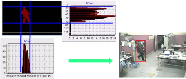
2. Compute the color histogram by kernel function, as shown in Fig. 4-3 (b) 3. ICs extracted.

4. Combined the histogram of color and ICs features, as shown in Fig. 4-4

0 10 20 30 40 50 0 10 20 30 40 50 0 0.2 0.4 0.6 0.8 1 (a) (b) (c) Fig. 4-3 (a) Human’s ROI (b) Kernel function (c) Histogram of color feature

Fig. 4-4 Color and ICA feature histogram

4.2 Kernel functions

The feature histogram based target representations are regularized by spatial masking with an isotropic kernel. The masking induces spatial-smooth similarity functions suitable for gradient-based optimization, hence, the target localization problem can be formulated using the basin of attraction of the local maxima [19].

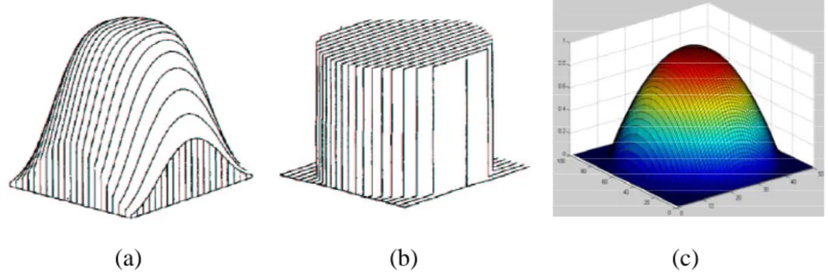
There are many kinds of kernel functions, such as Gaussian kernel, Flat kernel and Epanechnikov kernel. Let x be normalized pixel as location in the region defined as target model, then the Gaussian kernel, Flat kernel and Epanechnikov kernel [36] are defined as follows.

1. Gaussian kernel 2 1 1 ( ) exp( || ||) 2 2 k x x π = − (4.5) 2. Flat kernel (4.6) 3. Epanechnikov kernel 1 || || 1 ( ) 0 if x k x otherwise ≤ ⎧ = ⎨ ⎩ 2 3 (1 ) || || 1 ( ) 4 0 x if x k x otherwise ⎧ _{− ≤} ⎪ = ⎨ ⎪⎩ (4.7)

Fig. 4-5 (a) and (c) show that the Gaussian and Epanechnikov kernel are similar. They have highest value are the center distribution. If we take a looking the ROI of target model, the more closer to the center of ROI is containing more important pixels

Therefore, Gaussian and Epanechnikov kernel can regardless the boundary information and the accuracy will larger than flat kernel.

(a) (b) (c)

Fig. 4-5 (a) Gaussian kernel (b) flat kernel (c) Epanechnikov kernel

(a) (b) (c)

Fig. 4-6 (a) Target object (b) Kernel function (c) Target object and Kernel function

4.3 Mean-shift algorithm

In order to characterize the target, first a feature space is chosen. The reference target model is represent by normalized histogram q in the feature space. The target model can be considered as centered at the spatial location 0. In the subsequent frame, the candidate model is defined at location y, be expressed as p(y). We use Eq. 4.8 and Eq. 4.9 as our target and candidate model, respectively.

^ ^ 1... { }_{u u m} q= q ₌ (4.8) ^ 1 1 m u u q = =

∑

^ ^ 1... ( ) { _u( )}_{u m} p y = p y ₌ (4.9) ^ 1 1 m u u p = =

∑

The similarity value between and

^ p ^ q is defined as Eq. 4.10 (4.10) Target model

Let be normalized pixel locations in the region defined as the target model. The region is centered at 0. Here we use Epanechnikov kernel , using these weights increases the robustness of the density estimation since the peripheral pixels are the least reliable.

The function associates to the pixel at location

^ ^ [ ( ), ( )]p y q y ρ * 1... { }x_{i i= n} 2 : {1... } b R → m x* the index

b(x ) of its bin* re space. The probability of the featu e u=1…m

in the target model is then computed as

in the quantized featu r

^ ₂ * * 1 ( ) [ ( ) n i i u i q C k x δ b x u = =

∑

− ] (4.11)

where δ is the Kronecker delta function. The normalization constant C is derived by imposing the condition from where

^ 1 1 m u u q = =

∑

2 * 1 1 ( ) n i i C k x = =

∑

(4.12)

since the summation of delta functions for u=1…m is equal to one.

Candidate model

Let be the normalized pixel locations of the candidate model, center at y in the current frame. The normalization is succeed from the frame containing the target model. Here we use Epanechnikov kernel same as target model, but with bandwidth h,

* 1...

the probability of the feature u=1…m in the candidate model is given by 2 ^ 1 ( ) ( ) [ ( ) ] h n i h u i y x i p y C k b x u h δ = − =

∑

− (4.13) where 2 1 1 ( ) h h _n i i C y x k h = = −

∑

(4.14)

is the normalization constant. Note the does not depend on y because the pixel locations

h

C

i

x are organized in a regu y is one of the lattice nodes. The

bandwidth h defined the scale of the target candidate.

Similarity measure

The similarity function defines a distance among target model and candidate model. The Bhattacharyya coefficient, which evaluates the similarity of the target model and the candidate model, is defined as

lar lattice and

^ ^ ^ ^ 1 ( ) [ ( ), ] ( ) m u u u y p y q p y ρ ρ = ≡ =

∑

q^ (4. 15) ^ ^ ( ) 1 [ ( ), ] d y = −ρ p y q (4.16)

To find the location corresponding to the target in the current frame, the Bhattacharyya coefficient in Eq. (4.16) should be maximized as function of y which can be solved by running the mean-shift iterations.

Object localization

Color and ICs information were chosen as the features, however, the same framework can be used for texture and edges, or any combination of them. In the sequential, it is assumed that the following information is available: a. d detection and localization of the objects track in the initial frame b. Every objects periodic analysis accounting for possible updates of the target models due to significant changes in color.

Minimize the distance d(y) is equivalent to maximizing the Bhattacharyya coefficient ^ ( ) p y ^ 0

. The search for the new target location in the current frame starts at the location

y of the target in the previous frame. So the probabilities of the

candidate at location ^ ^ 0 1... {p_u(y )}_{u= m} ^ 0

y in the current frame have to be computed first. Using Taylor

expansion around the values

^ ^ 0 ( ) u p y ^ ^ ^ ^ ^ ^ ^ ^ 0 ^ ^ 1 1 0 1 1 [ ( ), ] ( ) ( ) 2 2 _{( )} m m u u u u u u u q p y q p y q p y p y ρ = = =

∑

+

∑

(4.17)

In order to minimize the distance d(y), the second term in Eq. 4.17 has to be the maximized, the first term being independent of y. The second term represents the density estimate computed kernel function at y in the current frame, with the data being weighted by Eq. 4.18. In this process, the kernel is recursively moved from current location i w 0 ^ y to new location ^ 1

y according to the relation. The distance

between ^ 1 y and ^ 0 y is mean-shift vector. ^ ^ ^ 1 0 [ ( ) ] ( ) m _u i u i u q w b p y δ = =

∑

x −u (4.18) 2 ^ 0 1 ^ 1 _^ 2 0 1 ( ) ( ) h h n _i i i i n _i i i y x x w g h y y x w g h = = − = −

∑

∑

(4.19) where g x( )= −k x'( ).

Fig. 4-7 Mean-shift algorithm flow chart Given the target model and its location

^ 1...

{ }q_{u u= m}

^ 0

y in the previous frame, set initial previous similarity value equal to 0, then the mean-shift algorithm is described as following,

1. Initialize the location of the target in the current frame with

^ 0 y , compute , and evaluate ^ ^ 0 1... {p_u(y )}_{u= m} ^ ^ ^ ^ ^ 0 0 1 [ ( ), ] ( ) m u u u p y q p y q ρ = =

∑

2. Derive the weights { }w_{i i=1...n}

h according toEq. 4.18.

3. Find the next location of the candidate according to Eq. 4.19. 4. Compute ,and evaluate

^ ^ 1 1... {p_u( )}y _{u= m} ^ ^ ^ ^ ^ 1 1 1 [ ( ), ] ( ) m u u u p y q p y q ρ = =

∑

^ ^ 0 [ (p y ), ]q ρ 5. If similarity_previous <= Do ^ ^ 1 1 1 ( ) 2 y ← y + ^ 0 y and similarity_previous = ^ ^ 0 [ (p y ), ]q ρ

Evaluate ^ 1 [ ( ), ] ^ p y q ρ and go to step 2. Otherwise ^ 0 ^ 1 y ← and break. y

4.4 ROI resizing

In real situation, human probably walk toward or keep away from camera, thus fixed ROI’s scale is not suitable because the ROI will contain some background pixels or only some parts of human.Consequently, it will influence tracking result shown in Fig. 4-8 and a similarity value smaller than a threshold value. Therefore, the ability to resize ROI’s scale is an important issue. In our system the ROI scale is adjusting every 100 frames.

Fig. 4-9 ROI resize flow chart

In order to adjust ROI scale adaptively, first we use temporal difference to find the foreground image and its position we do the temporal difference only in ROI’s regions. The dilation process is applied to gradually enlarge the boundaries of for ground pixel and link the broken boundary parts which obtain temporal difference. The projection of dilation image into x-axis and y-axis will produce the current width (width_current) and height (

is determ boundaries perfectly smaller than new ROI’ me current height e us the projection to an region.

ined then the ta of

^

u

q

) shown in Fig 4-10. Finally, the new ROI’s size ined with Eq. 4.20. Som times, the dilation process unable to link broken , th ward x-axis and y-axis will produce ROI actual hum So we will set the minimum size of ROI. After the s scale is determ rget model will be update, too. The update thod is use histogram shown in Eq. 4.21, where α is set to 0.6.

/ 2

/ 2 (4.20)

( )

( )

new previous current new previous current

height height height width width width

= +

⎧

⎨ _{= +}

⎩

arg _ (1 ) * _ * arg _

Fig. 4-10 X-axis and Y-axis image projection

In Fig. 4-11 and 4-12 show the ROI resize in fixed and active camera, respectively.

(a)

(b)

Fig. 4-11 Fixed camera condition (a) and (b) left is difference image. Right is after resize scale.

(a)

(b)

(c)

(e)

Fig. 4-12 Active camera condition. (a) original image (c-e) left are difference images. Right is ROI resizing scale image

4.5 Kalman filter

Fig. 4-13 Kalman filter flow chart

Fig. 4-13 shows the Kalman filter algorithm with use to predict the target location when the target is occluded with other object or if Bhattacharyya similarity value smaller than a threshold value (in this case we use threshold value equal to 0.65). if the Count smaller than 5, then it means object was occluded and the predicted

frames the target model histogram will be updated by Eq. 4.21.

In our system, the Kalman filter is integrated into mean-shift object tracking method. First, Kalman filter initialized by mean-shift target position. Second, the searching result of mean-shift is feedback as the measurement of Kalman filter and estimating its parameters.

1 ( ) ( ) ( ) ( ) k k k k k k X AX W a Z HX t V t b − = + ⎧ ⎨ _{= +} ⎩ (4.22)

We assume that and are Gaussian random variable with zero mean, so their probability density function are N[0,Q(t-1)] and N[0,R(t)], where the covariance matrix Q(t-1) and R(t) are referred to as the transition noise covariance matrix and measurement noise covariance matrix. Here

k

W Vk

[ , , , ]T k

X = x y Vx Vy is state of the system

at the moment k, [ , ]T k

Z = x y is measurement value of system state at the moment k.

x and V_x are the horizontal position and veloci . The value of state transition matrix A, measurement matrix H, process noise covariance matrix Q and measurement noise covariance matrix R list as following Eq. 4.23,

ty respectively 1 0 1 0 0 1 0 1 0 0 1 0 0 0 0 1 A ⎡ ⎤ ⎢ ⎥ ⎢ ⎥ = ⎢ ⎥ ⎢ ⎥ ⎣ ⎦ 1 0 0 0 0 1 0 0 0 0 1 0 0 0 0 1 Q ⎡ ⎤ ⎢ ⎥ ⎢ ⎥ = ⎢ ⎥ ⎢ ⎥ ⎣ ⎦ 1 0 0 0 1 0 0 1 0 0 0 1 H =⎡_⎢ ⎤_⎥ R=⎡_⎢ ⎤_⎥ ⎣ ⎦ ⎣ ⎦ (4.23)

The detail procedures of Kalman position prediction are listed bellow:

1. Predict the position of the target at moment k by kalman filter, and compute the prior error estimate covariance.

k ^ ^ ' ' 1 k k x =A x ₋ +w (a) (b) (4.24) ' 1 T k k P =AP A₋ +Q

2. Centered with predicted position

^ '

k

x , acquire the observation value Z_kaccording to Eq. 4.22(b).

3. Correct measurement with Kalman filter, compute the revision matrix and renew poster state estimation as well as posterior error estimate covariance.

' ' ( ) T T k k k K =P H HP H +R −1 (a) ^ ^ ^ ' ( ) k k k k k x = +x K Z −H x (b) k P (c) (4.25) Here Vx and Vy are x and y motions, respectively. In most application, we usually consider current and previous frame motion. If the moving object move in the same direction, using two frames motion to predict new position will obtain small error with respect to actual position. If the moving object moves in different direction use two frame motion are not good enough to represent because the predicted position. Here we consider more frames motion to get more accuracy, therefore we choose 5 frames motion’s average to get the more represent of moving direction.

f

/ f (4.26)

In both formulas, xi and yi are the horizontal and vertical coordinate of the target center respectively, ' (1 ) k k P = −K H ^ 1 1 ( ) / n f x x i i i n V α x x + − = + =

∑

− ^ 1 1 ( ) y y i i i n V α y y₋ = + =

∑

− x

α and α_y are proportional coefficients, f is the number of continuous frames. The distance between Kalman and mean-shift position are calculated by Euclidean distance.

In this section we use the position predicted by kalman filter compare with mean-shift. This comparison is helpful us to know the accuracy of the predicted position. We use Eq. 4-27 to calculate the error between mean-shift and Kalman filter.

^ 1 | | n i i i x x MAE n = − =

∑

(4.27)

Where xi is mean-shift position and x^ is predicted position by Kalman filter.

We do experiment both in indoor and outdoor environments. In the indoor environment, the human is not walking with a certain direction or path. Meanwhile, in the outdoor environment, the human is walking with the same direction.

(a)

(b)

(d)

Fig. 4-14 Indoor environment (a) frame 643 and 662 (b) frame 679 and 710 (c) frame 718 and 728 (d) frame 761 and 797

The MAE is calculated separately in x-direction and y-direction Fig.4-15 and Fig. 4-17 show the curves of x and y-position, where green line and blue line indicate mean-shift and Kalman filter prediction, respectively. The MAE position analysis uses 2 and 5-previous frames motion. Table 4-1 shows the MAE of 5-previous frame motion is smaller than 2-previous frame motion. Meanwhile, Table 4-2 shows that the MAE of 2 and 5-previous frame motion do not differ greatly. The reason is the MAE in Table 4-1 are generated from human that walking in several directions, thus using as much as possible frame to compute Kalman prediction will produce position better than 2-previous frame. But in the case of Table 4-2, the human is walking with the same direction , thus 2-previous frame enough to represent the Kalman prediction.

(b)

Fig. 4-15 (a) previous 2 frame motion left is x and right y position (b) previous 5 frame motion left is x and right y position

Table 4-1 MAE in different frame motion

X position error (pixel) Y position error (pixel) distance Previous 2 frame motion 18.25 3.74 18.9 Previous 5 frame motion 5.02 2.15 6.02

(a)

(c)

(d)

Fig. 4-16 Outdoor environment (a) frame 708 and 738 (b) frame 762 and 783 (c)frame 812 and 837 (d) frame 847 and 857

(a)

Fig. 4-17 (a) previous 2 frame motion left is x and right y position (b) previous 5 frame motion left is x and right y position

Table 4-2 MAE in different frame motion

X position error (pixel) Y position error (pixel) distance Previous 2 frame motion 3.98 3.6 5.89 Previous 5 frame motion 4.07 3.619 5.49

Chapter 5

Experimental

results

In this chapter, we will reveal the human detection and tracking system on active camera. Our algorithm was implemented on the platform of PC with Intel Core2 Quad 2.4GHz and 2GB RAM. Our algorithm was developed in Borland C++ Builder 6.0 on Window XP. Because our human detection and tracking system will run in real time video surveillance with an active pan-tilt-zoom camera, we should do some experiments to test its performance and stability under several kinds of environments.

In section 5.1, introduce the experimental environment. In section 5.2, we will experiment our kalman position predict and compare with mean-shift position and calculate their error by MAE (Mean absolute error). The kalman filter used in real-time situation to solve object occlusion problem. In section 5.3, we use experiment single object in the scenario. In section 5.4, we use experiment multiple objects in the scenario.

5.1 Environment setup

The environment of experimental locates in our laboratory. The complexity of the environment is enough to verify our system while tracking and detecting moving human. Fig. 5-1 show several images of our laboratory environment without zoom in/out operation. Fig. 5-2 shows several images for zoom in/out condition.

Fig. 5-1 Experimental environment

5.2 Kalman filter

The following two figures (Fig. 5-3 and Fig. 5-4) are compared under occlusion situation the difference between Kalman filter and no Kalman filter. In Fig. 5-3 We can observe a human pass the red screen will result the Bhattacharyya coefficient small than threshold so in frame 227 the mean-shift tracking will miss lock the object under occlusion problem. Fig. 5-4 Kalman filter was embedded in mean-shift algorithm the occlusion problem can be solve in frame 227 as shown in Table 5-1. We can also observe the object occluded for long time but the human was still be locked. Because the target object histogram be update so that kalman filter is not always be used in occlusion situation. Using histogram update idea in occlusion will increase tracking accuracy and precision.

There is one occlusion testing case in indoor environment. A man walking and then be occluded by a tall and long screen. In this situation the similarity measure will be drastically low so that the Kalman filter will be used to predict position.

Table 5-1 Predicted position

Frame number Similarity Object center 225 0.6874 (167,153) 226 0.6366 (165,153) 227 0.5933 (176,143) 259 0.6937 (112,118)

(a)

(b)

(c)

(d)

Fig. 5-3 Human tracking use mean-shift. (a) frame 194 and 206 (b) frame 225 and 234 (c) frame 243 and 246 (d) frame 255 and 277

(a)

(b)

(c)

(e)

Fig. 5-4 Human tracking use mean-shift and Kalman filter. (a) Frame 186 and 210 (b)Frame 224 and 227 (c) Frame 229 and 233 (d) Frame 255 and 263 (e)Frame 269 and 278

5.3 Active camera with single object experiment

In this section we experiment a single objects move in the scenario that active camera will smoothly trace the object. So there 5 topics to discuss one object in various situation that have different performance.

5.3.1 9 regions and 26 regions experiments

There are many methods to control the active camera direction, for example motion or position … etc. In this thesis we use position based method to control the camera pan/tilt directions. The image size is 320x240 so we divide into 9 and 25 regions. Every region implies a direction and speed so that the object in one of these regions the algorithm sends command to active camera tell it to pan/tilt.

In 9 regions, the speed of each regions have fixed speed and the speed was be stopped by stop command that means the pan/tilt angle was limited by stop command so in visual situation we can observe the camera stop and go repeat forever shown in Fig. 5-5. The stop and go phenomenon that result in observer uncomfortable. The 9 regions direction are show in Fig. 5-6. In real situation the object will be missed

In order to solve stop and go phenomenon, the regions of image divides into 25 regions shown in chap2 Fig. 2-5. Each regions have different speed and the stop command will not be used anymore so the we not limit the angle of pan/tilt. Thus stop and go problem will be solved show in Fig. 5-7.

Fig. 5-5 9 regions pan/tilt control

(a)

(b)

(d)

Fig. 5-6 Position based use 9 regions (a)frame 180, 244 and 272 (b)frame 345, 383 and 445 (c)frame 510, 560 and 564 (d)frame 567, 595 and 601

(a)

(b)

(c)

(e)

Fig. 5-7 Position based use 25 regions (a)frame 127, 189 and 213 (b)frame 241, 280 and 232 (c)frame 366, 385 and 418 (d)frame 473, 565 and 612 (e)frame 693, 775 and 843

5.3.2 Color spaces experiments

In section 5.2.1, there are two samples use HSV as color feature. We can observe this color space can focus on object shown in Fig. 5-7. So our experiment HSV is the main color space used on active camera. Because object walking in the scenario the lightness will result in object occurring essence change. In case of brighten occurred the object essence become different than original. Y’UV and RGB color space used to compare with HSV. In Fig. 5-8 is RGB color space used in our algorithm. In these figures we can track the object in the scenario smoothly, but the ROI position not always focus on object’s body. Sometimes it focuses on floor that the similarity values drastically down. The phenomenon in RGB color space has more sensitivity to lightness. In Fig. 5-9 the Y’UV color space is better than RGB.

(b)

(c)

(d)

Fig. 5-8 Choice RGB color space (a) frame 169, 215 and 283 (b) frame 328, 391 and 446 (c) frame 477, 506 and 537 (d) frame 623, 633 and 675

(b)

(c)

(d)

Fig. 5-9 Choice Y’VU color space (a) frame 134, 175 and 215 (b) frame 272, 306 and 325 (c) frame 401,449 and 477 (d) frame 497, 528 and 582

5.3.3 Using color and ICA features in human tracking

experiment

In this section, we will experiment the ICA features embedded in our mean-shift algorithm. In chapter 4, we have described how to combine color and ICA features in mean-shift algorithm. The purpose of ICA features is used to solve tracking miss problem. Target object is tracked by mean-shift algorithm when a background or nonhuman object has the same color with target object the tracking system maybe