國
立
交
通
大
學
網路工程研究所
碩
士
論
文
以適應性水閘資料匯集系統用於
長鏈狀無線感測網路之研究
Adaptive Lock Gate Designation Scheme for Data
Aggregation in Long-Thin Wireless Sensor Networks
研 究 生:莊哲熙
以適應性水閘資料匯集系統
用於長鏈狀無線感測網路之研究
學生: 莊哲熙 指導教授: 曾煜棋 教授 國立交通大學網路工程研究所碩士班 摘 要 因為物理環境的限制,近幾年來無線感測網路中,長鏈狀網路晉升為許多實 際部屬的拓樸結構。一般來說,長鏈狀拓樸是由多條長鏈狀分之所組成,每條分 之由多個感測點相連而成,而每個感測點都只有一個父節點。在長鏈狀拓樸下, 即使資料匯集可以降低無線感測網路中多餘的封包競爭,資料匯集還是會受到最 大封包資料量的限制。這篇論文提出長鏈分之中應該放置都個資料匯集點,稱作 水閘,負責匯集上游一般感測點的資料。這篇論文針對長鏈狀無線感測網路提出 一個適應性水閘指定方法,該方法在無線感測網路回報效率以及資料收集壅塞程 度中取得平衡,並且減輕無線感測網路中的漏斗效應。該方法更動態的調整水閘 的位置及數量以適應網路中隨時間變化的流量。實作結果顯示出適應性水閘指定 方法確實能改善長鏈狀網路的效能。 關鍵字:資料匯集,長鏈狀網路,普適計算,無線感測網路。Adaptive Lock Gate Designation Scheme for
Data Aggregation in Long-Thin Wireless Sensor Networks
Student: Che-Hsi Chuang
Advisor: Prof. Yu-Chee Tseng
Department of Computer Science
National Chiao-Tung University
ABSTRACT
Constrained by the physical environments, the long-thin (LT) topology has recently been promoted for many practical deployments of wireless sensor networks (WSNs). In general, an LT topology is composed of long branches of sensor nodes, where each sensor node has only one potential parent node toward the sink. Although data aggregation may alleviate excessive packet contention, constraints imposed by the maximum payload size of a packet severely limit the amount of sensor readings that may be aggregated along a long branch of sensor nodes. This paper argues that multiple aggregation nodes, termed lock gates, need to be designated along a branch to aggregate sensor readings sent from their respective upstream sensor nodes (up to the other upstream lock gate(s) and/or the end of the branch). The paper further describes an adaptive lock gate designation scheme for LT WSNs, which balances the responsiveness and the congestion of data collection, and mitigates the funneling effect. The scheme also dynamically adapts the designation of lock gates to accommodate the time-varying sensor reading generation rates of different sensor nodes. Experimental results demonstrate the effectiveness of the scheme.
Keywords: Data aggregation, long-thin network, pervasive computing, wireless sensor network.
誌謝
由衷地感謝曾煜棋教授這兩年來不辭辛勞的指導,讓我學到了很多寶貴的知 識跟經驗還有為人處事的方法,感謝實驗室的學長姐跟學弟妹,謝謝你們這兩年 多來的幫忙跟提攜,讓我得以順利完成學業,感謝爸媽辛苦地工作,讓我在求學 的過程中沒有後顧之憂,感謝瑞昱交大研發中心的同仁們,讓我學習了團隊合作 的技巧跟職場的經驗,感謝常常跟我一起打球的好朋友們,讓我除了學業之外能 有個豐富的生活,最後,特別感謝王友群學長跟林致宇學長,謝謝你們總是在我 心情低落時拉我一把,告訴我正確的人生態度跟處理事情的方法,真的讓我獲益 良多。 在此向大家獻上我誠摯地謝意跟祝福 莊 哲 熙 謹識於 國立交通大學網路工程研究所碩士班 中華民國九十七年七月Contents
Abstract i 誌謝 iii Contents iv List of Figures v 1 Introduction 1 2 Related Works 63 The Proposed ALT Scheme 8
4 Experimental Results 15
5 Conclusions 21
List of Figures
1.1 An example of LT WSNs ... 2 1.2 An LT WSN and its lock gates ... 3 3.1 Examples of moving next lock gates: (a) g1 moves g3 down- stream due to
T1 < Tmin, (b) g1 moves g2 to the branch node b due to T1 < Tmin, (c) g1 moves
g2 upstream due to T1 > Tmax, and (d) g1 moves g3 to node s due to T1 > Tmax.. 11
3.2 Counterexamples of moving next lock gates ... 12 4.1 The prototype of our LT WSN experiments ... 15 4.2 Three LT topologies in our experiments... 15 4.3 The change of the positions of lock gates when all sensor nodes
have the same sensor reading generation rate... 19 4.3 The change of the positions of lock gates when sensor nodes
have different sensor reading generation rates... 20
Chapter 1
Introduction
A wireless sensor network (WSN) consists of a sheer number of sensor nodes, where each sensor node is a wireless device that reports sensor readings of its surroundings to a sink node via multi-hop ad hoc communications. Such networks facilitate pervasive monitoring of the physical environments to enable applications such as habitat monitoring, smart home, and surveil-lance [5, 12, 13].
In recent research, the long-thin (LT) topology has been promoted for many practical applications of WSNs where the sensor deployment is sub-ject to environmental constraints [11]. For instance, a surveillance system of moving cars along streets, a monitoring system of carbon dioxide inside tun-nels, and a monitoring system of water quality within sewer lines are typical examples. Fig. 1.1(a) depicts the physical deployment of sensor nodes along streets, and Fig. 1.1(b) depicts its corresponding LT topology. In general, an LT topology is formed by a bunch of long ‘branches’ and each branch may be composed of tens or hundreds of nodes. For each sensor node along a branch, there exists only one potential parent node toward the sink. Branches are connected at branch nodes, and Fig. 1.1(b) shows an example where a branch node is denoted with double circles.
Let {s1, s2, · · · , sn} denote the node IDs of an LT WSN, where n is the
sensor node sink node
(a) physical deployment of sensor nodes along streets
(b) the corresponding LT topology
downstream upstream
branch 1
branch 2
branch node
Figure 1.1: An example of LT WSNs.
rooted at the sink, let di be the depth of node si from the sink. Assuming
that each sensor node in the LT WSN transmits one sensor reading to the sink without aggregating data, the network will incur Pni=1di transmissions
to collect all of the sensor readings. For instance, the LT WSN of Fig. 1.1 incurs 62 transmissions if no data aggregation is taken. Worse, an LT WSN may exhibit the funneling effect where the hop-by-hop traffic over a long branch results in an increase in transit traffic intensity, collision, congestion, packet loss, and energy drain as packets move closer toward the sink [2].
Now consider the following aggregation scheme. The leaf nodes start transmitting their sensor readings first. Each intermediate node waits to aggregate its own sensor reading with the (aggregated) sensor reading(s) sent from its child(ren), and then forwards the aggregated packet toward the sink. Such scheme may result in only n packet transmissions in the network, assuming that successively aggregated sensor readings could be loaded into one big packet. For instance, the LT WSN of Fig. 1.1 may incur only 12 transmissions using such aggregation scheme. Fewer transmissions benefit WSNs by conserving energy and reducing contention.
Although such aggregation maximally reduces the number of transmis-sions in an LT WSN, constraints imposed by the maximum payload size Lmax
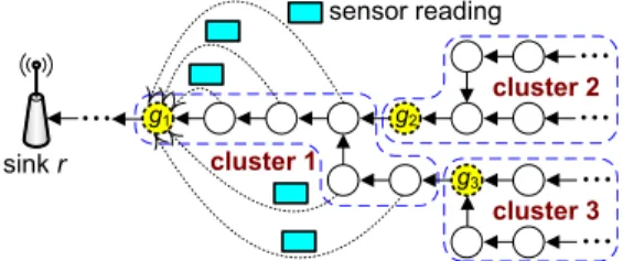
g1 sink r g2 g3 cluster 1 cluster 3 cluster 2 sensor reading
Figure 1.2: An LT WSN and its lock gates.
of a packet and the compression ratio δ (0 < δ ≤ 1) make such scheme im-practical for an LT topology where a node may only aggregate up to bLmax
δ c
bytes of sensor readings, while the total data size of sensor readings gener-ated by sensor nodes of a (long) branch in an LT topology may well exceed this bound.
To mitigate the funneling effect and to comply with the maximum payload size, the paper suggests that along a branch, multiple aggregation nodes, termed lock gates1 in the paper, need to be designated, where each lock gate
aggregates its own sensor reading with all of the sensor readings sent from its upstream sensor nodes (up to immediate, upstream lock gate(s) or the end of the branch) subject to the bLmax
δ c bound. For instance, as shown in
Fig. 1.2, assuming Lmax is 3 bytes, δ is 0.5, and the size of sensor readings is
1 byte, we designate one lock gate every six sensor nodes so that lock gate
g1 aggregates its own sensor reading with those from its five upstream nodes
into one aggregated packet2. Similarly, this can be done by lock gates g
2 and
g3. Such an aggregated packet (of maximum payload size Lmax) is said to be
completely filled up with sensor readings and thus can be forwarded to the sink without being aggregated with any other sensor readings along the way. Another benefit of the above lock gate design is that it actually reduces
1We were inspired by the lock gates used in canals to withstand the water pressure
arising from the level difference between adjacent pounds. In the context of LT WSNs, (ir-regular) network traffic from sensor readings corresponds to water pressure, which should be regulated to mitigate funneling effect, for instance.
2Here we assume that there is no ‘protocol overhead’ (or packet header/trailer) so that
contention among traffic by spatially separating areas where packets are transmitted. In the above example, since lock gates g2 and g3 will hold their
transmissions until enough sensor readings from the corresponding upstream nodes have been collected, the members of the cluster led by lock gate g1
can transmit their sensor readings to g1 with little or even no interference
coming from clusters of lock gates g2 and g3.
However, since sensor nodes may generate sensor readings at different
rates, each lock gate may wait for a different amount of time to completely
fill up an aggregated packet of size Lmax. Let λj denote the sensor reading
generation rate (bytes/second) of sensor node sj. Let C(gi) denote the clus-ter of nodes containing lock gate gi and its upstream sensor nodes, up to
immediate, upstream lock gate(s) or the end of the branch. Assuming that each λj is a constant and the WSN operates at a steady state, the following
equation indicates the amount of time Ti taken by lock gate gi to completely
fill up an aggregated packet of size Lmax.
Ti× X sj∈C(gi) λj × δ = Lmax. (1.1)
When Ti is large, the sink is expected to wait for a longer time to receive
an aggregated packet from lock gate gi, which increases the response time
of monitoring. Large Ti may imply either the size of C(gi) is small or the
total sensor reading generation rate of the sensor nodes in C(gi) is low, or
both. In contrast, small Ti may imply either the size of C(gi) is large or the
total sensor reading generation rate of the sensor nodes in c(gi) is high, or
both. This may result in too many packet transmissions and thus congest the network.
This paper proposes an adaptive lock gate designation scheme, termed
ALT, to facilitate effective data aggregation in LT WSNs. Given a pair of
time thresholds, (Tmin, Tmax), specified by the application of an LT WSN to
caused by transmitted packets, ALT designates lock gates in an LT WSN such that for each lock gate gi, Tmin ≤ Ti ≤ Tmax. Specifically, when sensor reading
generation rate λi varies over time, ALT dynamically adjusts the positions
of lock gates (and thus the definitions of clusters) to balance response time and congestion. To the best of our knowledge, this is the first effort that addresses efficient data aggregation in LT WSNs.
The remainder of this paper is organized as follows. The next section describes related work. Section 3 describes our ALT scheme. Section 4 reports our prototyping efforts and experimental results. Section 5 concludes the paper.
Chapter 2
Related Work
The subject of data aggregation in WSNs has been extensively studied. How-ever, most research efforts used either a tree-based or a cluster-based archi-tecture to aggregate data in WSNs, and none of them considered the LT topology.
Tree-based aggregation schemes use the shortest path routing tree, and focus on how to choose a good routing metric based on data attributes to facilitate data aggregation. For instance, the work of [6, 8] proposed a data-centric approach to select an appropriate path to reduce energy consumption. In addition, the work of [1] built an aggregation tree according to the energy consumption of sensor nodes. Each node predicts the energy consumption of its potential parents and selects the one that can be left with the most energy as its parent. In contrast, in LT WSNs, there exists at most one route from a sensor node to the sink (i.e., each sensor node has at most one potential parent node toward the sink) so that existing solutions may not be directly applied.
In comparison, cluster-based aggregation schemes group sensor nodes into clusters and perform aggregation within each cluster. For instance, in LEACH [4] and PEGASIS [10], sensor nodes relay their sensor readings to the corresponding cluster heads, which are assumed to be able to commu-nicate directly with the sink. However, this assumption is not valid in LT
WSNs. In addition, HEED [14] groups sensor nodes such that sensor nodes within a cluster are single-hop away from the cluster head. However, in an LT WSN, sensor nodes within a cluster are located along a long branch which are multi-hop away from their cluster head. SCT [15] proposed a ring-sector division clustering scheme, where sensor nodes in the same section are assem-bled into one cluster. Clearly, this approach cannot be used for LT WSNs. Reference [3] considered aggregating data without maintaining any structure. It proposed a MAC protocol and studied the impact of randomized wait time to improve aggregation efficiency. However, this scheme may increase packet delays in LT WSNs.
Chapter 3
The Proposed ALT Scheme
The LT topology is first proposed in [11]. We model an LT WSN as graph
G = (V, E), where V = {r} ∪ S contains the sink r and the set of sensor
nodes S, and E contains all of the communication links. The topology of G is represented as a tree rooted at sink r. Each sensor node sj ∈ S has a sensor
reading generation rate of λj, which may vary over time during the network
operation. A sensor node is called a branch node if it has more than one child in G. Fig. 1.2 depicts an example of LT WSNs, where three clusters are identified and nodes g1, g2, and g3 are designated as lock gates.
Given an LT WSN, ALT first randomly groups sensor nodes into several non-overlapping clusters covering the entire network, and designates their corresponding lock gates. Note that the sensor node closest to the sink is always designated as a lock gate. On generating one sensor reading, each regular sensor node will send the reading to its corresponding lock gate. Each lock gate gi then collects the sensor readings from the sensor nodes
within its cluster C(gi). After collecting enough sensor readings that can be
aggregated to fill up one packet of maximum payload size Lmax, lock gate gi sends the packet toward the sink. To reduce the latency of waiting to
aggregate enough sensor readings to fill up one packet of maximum payload size Lmax, lock gate gi may dynamically adjust its cluster according to the
to Eq. (1.1)). When Ti is below a given lower-bound threshold Tmin, the
total sensor reading generation rate within this cluster (i.e., Psj∈C(gi)λj)
becomes too high, and aggregated packets will be sent to the sink more often. In this case, lock gate gi ‘shrinks’ its cluster by excluding certain sensor
nodes to lower the total sensor reading generation rate. In contrast, when
Ti is above a given upper-bound threshold Tmax, the total sensor reading
generation rate within this cluster becomes too low, and the monitoring quality degrades. In this case, lock gate gi ‘expands’ its cluster by including
more sensor nodes to lower the latency of generating aggregated packets. Note that within each cluster C(gi), the sensor readings sent from each sensor sj ∈ C(gi) may be relayed to lock gate gi in a pipeline manner subject to the
contention of wireless transmissions. Thus, right before lock gate gisends out
each (completely filled) aggregated packet toward the sink, the percentage of sensor readings received from sensor sj within this packet is approximately
equal to P λj
sk∈C(gi)λk. In other words, ALT ensures that the amount of reported
sensor readings from each sensor node is fairly proportional to the sensor reading generation rate of that sensor node.
Before describing ALT in details, we first define the terms used in the remainder of the paper. A lock gate gk is called a next lock gate of lock
gate gi if gk is an immediate upstream lock gate of gi. In this case, gi is the previous lock gate of gk. For example, in Fig. 1.2, g2 is a next lock gate of g1 while g1 is a previous lock gate of g2. Note that each lock gate may have
multiple next lock gates but at most one previous lock gate. In addition, a lock gate is called a leaf lock gate if it has no next lock gate; otherwise, it is a non-leaf lock gate.
From an initial lock gate designation, lock gates execute ALT
asyn-chronously, while coordinating with previous and next lock gates. Each lock
gate gi measures its current Ti value, ‘moves’ one of its next lock gates (if
necessary) downstream or upstream by one-hop, and recalculates its Ti value.
Specif-ically, for each non-leaf lock gate gi, two cases are considered:
Case of Ti < Tmin: In this case, lock gate gi shrinks its cluster by first
querying each of its next lock gates gk for its Tk value. If lock gate gk is also
in the state of adjusting its own next lock gates, lock gate gk will reply to
lock gate gi that itself is busy; otherwise, lock gate gk will reply to lock gate gi for its Tk value. If lock gate gi finds that all of its next lock gates are busy,
it will wait for a ∆t time and try again. Otherwise, lock gate gi sends a pull
message to the next lock gate gkwhose parent node, say, sj on graph G is not
a branch node and whose Tk value is the largest. On receiving such a pull
message, lock gate gk designates sensor node sj to become a new lock gate
and clears itself as a lock gate. In this case, the old cluster c(gk) disappears
and a new cluster c(sj) appears. For convenience, we use the term ‘move’ to
represent such an operation. However, in the case that lock gate gi cannot
find such a next lock gate (which means that the parent nodes of all of its next lock gates on G are branch nodes), the next lock gate gk that has the
maximum Tk value is asked to move one-hop downstream. These operations
are repeated until lock gate gi computes that Ti ≥ Tmin.
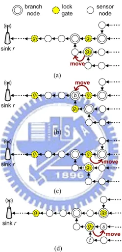
Fig. 3.1(a) gives an example, where g1 wants to adjust one of its next lock
gates g2 and g3. Since the parent node of lock gate g2 is a branch node, lock
gate g3 will be asked to move downstream. When all of the parent nodes of
all of its next lock gates are branch nodes, as shown in Fig. 3.1(b), assuming
T2 > T3, ALT will ask lock gate g2 to move to node b.
To avoid excluding too many sensor nodes when shrinking a cluster, which may make its Ti value increase drastically, ALT avoids moving a next lock
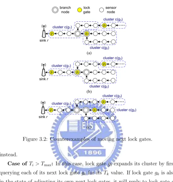
gate whose parent node on G is a branch node as much as possible. Fig. 3.2(a) shows a counterexample, where we assume T2 > T3. If g1 simply moves
its next lock gate whose Ti value is the largest, g2 will be asked to move
downstream, as shown in Fig. 3.2(b). In this case, the size of cluster c(g1)
will drastically decrease from 7 to 3. Moreover, the size of cluster c(g2) will
g1 sink r g2 g3 b (b) g1 sink r g2 (a) g1 sink r g2 (c) g1 sink r g2 (d) move move g3 move g3 g3 move t s branch node lock gate sensor node
Figure 3.1: Examples of moving next lock gates: (a) g1moves g3 downstream
due to T1 < Tmin, (b) g1 moves g2 to the branch node b due to T1 < Tmin, (c) g1 moves g2 upstream due to T1 > Tmax, and (d) g1 moves g3 to node s due
g1 sink r (a) g2 branch node lock gate sensor node g3 cluster c(g1) cluster c(g2) cluster c(g3) g1 sink r g2 g3 cluster c(g1) cluster c(g2) cluster c(g3) (b) g1 sink r (c) g3 cluster c(g1) cluster c(g2) cluster c(g3) g2
Figure 3.2: Counterexamples of moving next lock gates. instead.
Case of Ti > Tmax: In this case, lock gate gi expands its cluster by first
querying each of its next lock gate gk for its Tk value. If lock gate gk is also
in the state of adjusting its own next lock gates, it will reply to lock gate gi
that itself is busy; otherwise, it will reply to lock gate gi for its Tk value. If
lock gate gi concludes that all of its next lock gates are busy, it will wait for
a ∆t time and try again. Otherwise, lock gate gi sends a push message to
ask the next lock gate gk that is not a branch node and has the minimum Tk value to move one-hop upstream. In the case that lock gate gi cannot
find such a next lock gate (which means that all of its next lock gates are branch nodes), the next lock gate gk that has the minimum value of Tk will
be asked to move upstream. These operations are repeated until lock gate gi
Fig. 3.1(c) gives an example, where g1 wants to adjust one of its next lock
gates g2 and g3. Since lock gate g2 is not a branch node, it will be moved
upstream. When all of the next lock gates are branch nodes, as shown in Fig. 3.1(d), assuming that T3 < T2, ALT will ask lock gate g3 to move to
node s. Note that in the latter case, g3, t, and some of t’s subsequent nodes
will be merged into the cluster c(g1).
Similar to shrinking a cluster, to avoid including too many sensor nodes when expanding a cluster, which may make its Ti value decrease drastically,
ALT avoids moving a next lock gate that is a branch node as much as possible. Fig. 3.2(a) shows a counterexample, where we assume T2 < T3. If g1 simply
moves its next lock gate whose Ti value is the smallest, g2 will be asked to
move upstream, as shown in Fig. 3.2(c). In this case, the size of cluster c(g1)
will drastically increase from 7 to 12. Moreover, the size of cluster c(g2) will
drastically decrease from 8 to 3. In fact, ALT will move g3 upstream instead.
For each leaf lock gate gi, it will be moved according to the push or pull
request from its previous lock gate. Moreover, two special cases must be considered. First, if gi is asked to move upstream but itself is already a leaf
node in G, then gi will simply clear itself as a lock gate and become a regular
sensor node. In this case, the total number of lock gates in the network decreases by one. Second, if gi is asked to move downstream but finds that Ti < Tmin, it will do as requested and select one leaf node, say, sj in its cluster
and designate sj as a new lock gate. In this case, the total number of lock
gates in the network increases by one.
To prevent lock gates from oscillating or moving back and forth between two adjacent nodes, each lock gate gi should maintain a short list recording
its past positions on G. If lock gate gi finds that it has moved between two
adjacent nodes (termed oscillating nodes) more than β times and its previous lock gate still asks it to move to one of the oscillating nodes, it enters the
oscillating state. In this case, lock gate gi will notify its previous lock gate to
state if its previous lock gate asks it to move to one non-oscillating node or a pre-set oscillating timer expires.
When each sensor node has a fixed sensor reading generation rate, the lock gates designated by ALT will eventually stabilize and converge (from an initial random designation) due to the following two factors. First, a lock gate can only move its next lock gates but cannot move its previous lock gate. In this case, clusters stabilize in sequence from the downstream direction to the upstream direction. Second, ALT employs the oscillation avoidance technique described in the previous paragraph.
We now analyze and compare the latency of sending packets from each sensor node sj to sink r with and without applying ALT. Assume that sj is
located within cluster C(gi). Let Dj,i and Di,rbe the latency of a packet from
sensor node sj to lock gate gi and from lock gate gi to sink r, respectively.
When no lock gate is used, the latency of a packet from sensor node sj to
sink r is DNL
j,r = Dj,i+ Di,r. In contrast, by using ALT, since lock gate gi will
send its aggregated packet to sink r after Ti, we have DL
j,r ≤ Dj,i+ Ti + Di,r= DNLj,r + Ti. (3.1)
By combining Eqs. (1.1) and (3.1), ALT can only increase the packet latency as follows: DL j,r − Dj,rNL ≤ Lmax δ ×Psk∈C(gi)λk .
Figure 4.1: The prototype of our LT WSN experiments.
...
...
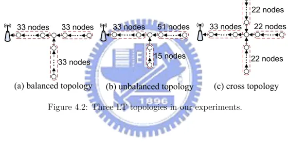
33 nodes
33 nodes
(a) balanced topology (b) unbalanced topology (c) cross topology
...
33 nodes...
...
33 nodes 15 nodes 51 nodes...
...
...
33 nodes 22 nodes 22 nodes...
...
22 nodesFigure 4.2: Three LT topologies in our experiments.
Chapter 4
Experimental Results
In this section, we describe our prototyping efforts and experimental results. We deploy one hundred sensor nodes and one sink node to collect data from
the environment, as shown in Fig. 4.1. Each sensor node contains a Jennic JN5139 chip [7], which is a low power, wireless micro-controller supporting the IEEE 802.15.4 protocol. Each sensor node has a communication distance of approximately 30 centimeters (cm). We place two adjacent nodes with a distance of 15 cm to make the network connected. Three LT topologies are deployed in our experiments. The balanced topology (Fig. 4.2(a)) has two branches, each with 33 nodes. The unbalanced topology (Fig. 4.2(b)) has two branches, one containing 51 nodes while the other containing 15 nodes. The cross topology (Fig. 4.2(c)) has three branches, each with 22 nodes. We compare ALT against the brute force (BF) and the fixed lock gate selection (FLS) schemes using these three network topologies. BF does not apply any aggregation, where each sensor node simply relays the sensor readings from its upstream nodes to the sink. In FLS, each branch node is designated as a lock gate and we do not adjust the designation of lock gates during the experiments.
The packet size of a sensor reading is 15 bytes, which contains a header of 12 bytes (according to the IEEE 802.15.4 standard [9]) and a payload of 3 bytes. Each sensor node reports its sensor reading every ∆sseconds,
where ∆s is randomly selected from [(1 − α) × 10, (1 + α) × 10] and it may
be changed every 30 seconds. Note that when α = 0, the sensor reading generation rate (i.e., λi) is 0.3 bytes/second. We adopt a simple aggregation
scheme by removing the packet headers of all of the received sensor readings and then concatenating their payloads into one single packet. In this way, we have δ = 1. In our experiment, we set Lmax as 118 bytes, which is the
maximum payload size of a packet defined in the IEEE 802.15.4 standard. The total experiment time is 10 minutes. In the experiments of running ALT, the measurement of messages sent by sensor nodes includes all of the control messages (e.g., query, reply, push, and pull) used to adjust the designation of lock gates. Other parameters used in the experiments are set as follows:
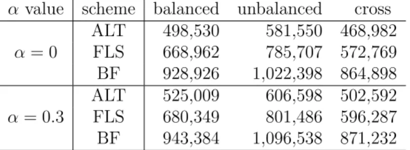
Table 4.1: Comparison on the total amount of messages (in bytes) sent by sensor nodes in different network topologies.
α value scheme balanced unbalanced cross ALT 498,530 581,550 468,982 α = 0 FLS 668,962 785,707 572,769 BF 928,926 1,022,398 864,898 ALT 525,009 606,598 502,592 α = 0.3 FLS 680,349 801,486 596,287 BF 943,384 1,096,538 871,232
Table 4.1 shows the total amount of messages sent by sensor nodes in different network topologies. BF suffers from the highest amount of messages because it does not apply any aggregation. By dynamically adjusting the positions of lock gates according to the network condition, ALT enjoys a lower amount of messages compared with FLS. It can be shown that when α = 0, ALT saves 18.1% to 26.0% and 43.1% to 46.3% of message transmission compared with FLS and BF, respectively. When α = 0.3, ALT saves 15.7% to 24.3% and 42.3% to 44.7% of message transmission compared with FLS and BF, respectively. These results show the effectiveness of ALT. Note that the three schemes all suffer from the highest amount of messages under the unbalanced topology, because this topology has the longest branch (with 51 nodes). In addition, when α = 0.3, the amount of messages increases because sensor nodes generate more sensor readings. In this case, since the network is not stable, ALT needs to generate more control messages to adjust the designation of lock gates.
Table 4.2 shows the total number of packets sent by sensor nodes in dif-ferent network topologies. When sensor nodes transmit more packets, the network could be more seriously congested. BF makes the sensor nodes transmit the most number of packets, since it does not aggregate any sensor reading. ALT enjoys the smallest number of packets among all three schemes because it adaptively clusters sensor nodes and aggregates their packets ac-cordingly. We observe that when α = 0, ALT saves 59.1% to 72.3% and
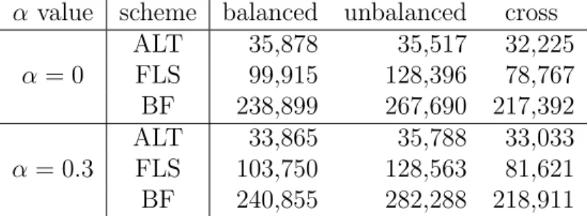
Table 4.2: Comparison on the total number of packets sent by sensor nodes under different network topologies.
α value scheme balanced unbalanced cross ALT 35,878 35,517 32,225 α = 0 FLS 99,915 128,396 78,767 BF 238,899 267,690 217,392 ALT 33,865 35,788 33,033 α = 0.3 FLS 103,750 128,563 81,621 BF 240,855 282,288 218,911
85.0% to 86.7% of packets compared with FLS and BF, respectively. When
α = 0.3, ALT saves 59.5% to 72.2% and 84.9% to 87.3% of packets
com-pared with FLS and BF, respectively. These results demonstrate that ALT significantly reduces the number of packets sent by sensor nodes, which can greatly alleviate the network congestion.
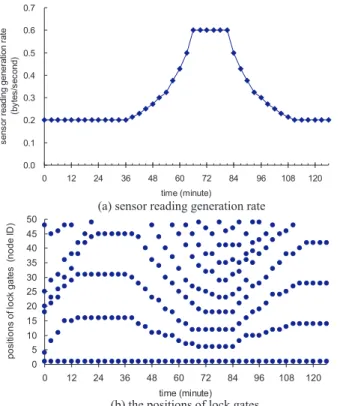
To demonstrate the adaptability of ALT to varying sensor reading gener-ation rates, we deploy a sink (of ID 0) and a line of 50 sensor nodes (of IDs 1 to 50), where the node with ID 1 is the most downstream sensor node. The duration of the experiment is 126 minutes and we measure the (changing) number of lock gates and their designation (or positions) over time. All of the sensor nodes have the same sensor reading generation rate (λ), which changes every 3 minutes as shown in Fig. 4.3(a). For instance, starting at 0.2 byte/second, λ remains at the same rate until the 36th minute, increases to 0.6 bytes/second at the 66th minute, remains at the same rate until the 81st minute, and then decreases. Fig. 4.3(b) depicts the changing designa-tion of lock gates, as dots, over time. For instance, at 0th minute, there are 6 lock gates randomly designated at nodes of IDs 1, 4, 18, 20, 25, and 48. Before the 36th minute, λ is not changed and thus the positions of lock gates stabilize at nodes of IDs 1, 16, 31, and 45 at the 24th minute. As λ increases, the size of the clusters decreases and the number of lock gates increases ac-cordingly. Between the 66th to the 81st minutes, λ remains stable and thus the positions of lock gates are only slightly adjusted. For instance, at the
72nd minute, 8 lock gates are designated at nodes of IDs 1, 6, 12, 18, 25, 32, 38, and 47. After the 81st minute, as λ decreases, the number of lock gates also decreases and the size of clusters increases. After the 117th minute, the position of lock gates remains stable because λ becomes stable. Since all of the sensor nodes have the same λ value, we also observe that the distance between any two adjacent lock gates is quite similar at most time instances. Such a phenomenon is more visible when the number of lock gates is smaller. These observations demonstrate that ALT can efficiently adjust the size of each cluster (and designate the lock gate accordingly) based on the traffic sent from the sensor nodes in that cluster.
0.0 0.1 0.2 0.3 0.4 0.5 0.6 0.7 0 12 24 36 48 60 72 84 96 108 120 time (minute) s e n s o r re a d in g g e n e ra tio n ra te (b y te s /s e c o n d ) 0 5 10 15 20 25 30 35 40 45 50 0 12 24 36 48 60 72 84 96 108 120 time (minute) p o s it io n s o f lo ck g a te s (n o d e ID )
(a) sensor reading generation rate
(b) the positions of lock gates
Figure 4.3: The change of the positions of lock gates when all sensor nodes have the same sensor reading generation rate.
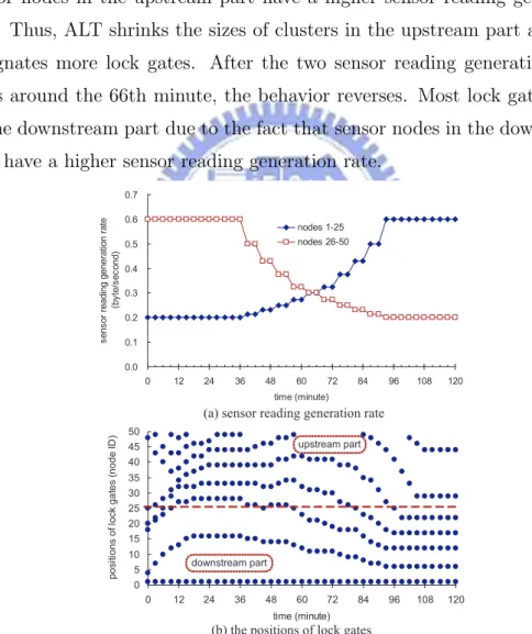
Using the same network topology in the previous experiment, we also demonstrate the adaptability of ALT when sensor nodes have different sensor reading generation rates (λ). Specifically, the λ value of sensor nodes of IDs 1
to 25 increases while that of sensor nodes of IDs 26 to 50 decreases over time, as shown in Fig. 4.4(a). For convenience, we use the terms ‘downstream part’ and ‘upstream part’ to represent the sensor nodes of IDs 1 to 25 and of IDs 26 to 50, respectively. The duration of the experiment is 120 minutes. Beginning with the same random lock gate designation as the previous experiment, Fig. 4.4(b) shows the positions of lock gates over time. We observe that before the 60th minute, most lock gates are located at the upstream part because sensor nodes in the upstream part have a higher sensor reading generation rate. Thus, ALT shrinks the sizes of clusters in the upstream part and thus designates more lock gates. After the two sensor reading generation rates cross around the 66th minute, the behavior reverses. Most lock gates move to the downstream part due to the fact that sensor nodes in the downstream part have a higher sensor reading generation rate.
0.0 0.1 0.2 0.3 0.4 0.5 0.6 0.7 0 12 24 36 48 60 72 84 96 108 120 time (minute) s e n s o r re a d in g g e n e ra tio n ra te (b y te /s e c o n d ) nodes 1-25 nodes 26-50 0 5 10 15 20 25 30 35 40 45 50 0 12 24 36 48 60 72 84 96 108 120 time (minute) p o s it io n s o f lo c k g a te s (n o d e ID )
(a) sensor reading generation rate
(b) the positions of lock gates
downstream part
upstream part
Figure 4.4: The change of the positions of lock gates when sensor nodes have different sensor reading generation rates.
Chapter 5
Conclusions
Many realistic WSN applications dictate the deployment of an LT topology which demands new data aggregation schemes. The paper described the ALT lock gate designation scheme which (1) designates multiple lock gates within an LT WSN to regulate data aggregation and (2) adapts the designation of lock gates dynamically in response to changing sensor reading generation rates of sensor nodes. ALT balances the responsiveness and the congestion of data collecting, and mitigates the funneling effect by regulating (aggregated) data that could be transmitted downstream and spatially separating areas where packets are transmitted. Using the Jennic JN5139 wireless micro-controllers, we evaluated the performance of ALT via several experiments of prototyped LT WSNs. Experimental results demonstrated the merits of ALT. Research is in progress to further analyze and quantify the impact of designating multiple lock gates on MAC layer contention and packet loss.
Bibliography
[1] A. F. Harris III, R. Kravets, and I. Gupta. Building trees based on aggregation efficiency in sensor networks. ACM Ad Hoc Networks, 5(8):1317–1328, 2007. [2] G. S. Ahn, S. G. Hong, E. Miluzzo, A. T. Campbell, and F. Cuomo. Funneling-MAC: a localized, sink-oriented MAC for boosting fidelity in sensor networks. In ACM International Conference on Embedded Networked Sensor Systems, pages 293–306, 2006.
[3] K. W. Fan, S. Liu, and P. Sinha. Structure-free data aggregation in sensor networks. IEEE Transactions on Mobile Computing, 6(8):929–942, 2007. [4] M. J. Handy, M. Haase, and D. Timmermann. Low energy adaptive clustering
hierarchy with deterministic cluster-head selection. In IEEE International
Workshop on Mobile and Wireless Communications Network, pages 368–372,
2002.
[5] S. Helal, W. Mann, H. El-Zabadani, J. King, Y. Kaddoura, and E. Jansen. The gator tech smart house: a programmable pervasive space. IEEE Computer, 38(3):50–60, 2005.
[6] C. Intanagonwiwat, R. Govindan, and D. Estrin. Directed diffusion: a scalable and robust communication paradigm for sensor networks. In ACM
Interna-tional Conference on Mobile Computing and Networking, pages 56–67, 2000.
[7] Jennic microcontrollers.
[8] B. Krishnamachari, D. Estrin, and S. Wicker. The impact of data aggregation in wireless sensor networks. In IEEE International Conference on Distributed
Computing Systems Workshops, pages 575–578, 2002.
[9] LAN/MAN Standards Committee of the IEEE Computer Society. IEEE Std 802.15.4-2003, Wireless medium access control (MAC) and physical layer (PHY) specifications for low-rate wireless personal area networks (LR-WPANs). IEEE, 2003.
[10] S. Lindsey and C. S. Raghavendra. PEGASIS: power-efficient gathering in sensor information systems. In IEEE Aerospace Conference, pages 1125–1130, 2002.
[11] M. S. Pan, H. W. Fang, Y. C. Liu, and Y. C. Tseng. Address assignment and routing schemes for ZigBee-based long-thin wireless sensor networks. In
[12] R. Szewczyk, E. Osterweil, J. Polastre, M. Hamilton, A. Mainwaring, and D. Estrin. Habitat monitoring with sensor networks. Communications of the
ACM, 47(6):34–40, 2004.
[13] Y. C. Tseng, Y. C. Wang, K. Y. Cheng, and Y. Y. Hsieh. iMouse: an in-tegrated mobile surveillance and wireless sensor system. IEEE Computer, 40(6):60–66, 2007.
[14] O. Younis and S. Fahmy. Distributed clustering in ad-hoc sensor networks: a hybrid, energy-efficient approach. In IEEE INFOCOM, pages 629–640, 2004. [15] Y. Zhu, R. Vedantham, S. J. Park, and R. Sivakumar. A scalable correlation aware aggregation strategy forwireless sensor networks. In IEEE International