效用函數，風險趨避與避險分析---理論模型與應用(I)

行政院國家科學委員會專題研究計畫 成果報告

效用函數，風險趨避與避險分析：理論模型與應用(I)

計畫類別： 個別型計畫 計畫編號： NSC91-2416-H-009-018- 執行期間： 91 年 08 月 01 日至 92 年 07 月 31 日 執行單位： 國立交通大學經營管理研究所 計畫主持人： 李正福 共同主持人： 李昭勝 計畫參與人員： 吳志強 柯玫伶 蕭亦融 楊華勝 洪祥玲 余碧珠 謝碧鳳 報告類型： 精簡報告 報告附件： 出席國際會議研究心得報告及發表論文 處理方式： 本計畫可公開查詢

中 華 民 國 92 年 10 月 28 日

行政院國家科學委員會補助專題研究計畫 - 成果報告

計畫名稱: 效用函數、風險趨避與避險分析: 理論模型與應用

Utility Function, Risk Aversion and Hedging Analysis:

Theory Methods and Application

計畫類別：V 個別型計畫 □ 整合型計畫

計畫編號：NSC 91-2416-H-009-018

執行期間：91 年 8 月 1 日至 92 年 7 月 31 日

計畫主持人：李正福

共同主持人：李昭勝

計畫參與人員：

吳志強、洪祥玲、余碧珠、謝碧鳳、柯玫伶、蕭亦融、

楊華勝

成果報告類型(依經費核定清單規定繳交)：V 精簡報告 □完整報告

本成果報告包括以下應繳交之附件：

□赴國外出差或研習心得報告一份

□赴大陸地區出差或研習心得報告一份

V 出席國際學術會議心得報告及發表之論文各一份

□國際合作研究計畫國外研究報告書一份

處理方式：除產學合作研究計畫、提升產業技術及人才培育研究計畫、

列管計畫及下列情形者外，得立即公開查詢

□ 涉及專利或其他智慧財產權，□一年□二年後可公開查詢

執行單位：國立交通大學財務金融所

中 華 民 國 92 年 10 月 27 日

I. 中英文摘要及關鍵詞(keywords)

(一) 中文摘要

財務理論乃依據 utility function 和 risk aversion 理論導出。依據 utility function 和 risk aversion 理論可導出的理論包括 capital asset pricing model、option pricing model、與避險理論。因此，在這個研究計劃的第一階段時， 我們深入探討 Gibbons and Brown 於 1985 年所提出的 Risk Aversion parameter 的估計方法，並更進一步擴展其理論與實務應用的範疇。在第二階段時，我們從文 獻方面著手，探討各種可應用於 hedging 和估計 hedge ratio 的 utility

functions。同時也探討各種不同的 hedge ratio models 與其估計方法。最後，本 計劃透過結合實際市場資料的方法，將 hedging theory 和 hedge ratio 的估計納 入成為評估 Risk Aversion parameter 的重要環節。在這個計劃中，我們應用到的 實際市場資料包括市場投資報酬率(market rate of return)，無風險報酬率 （risk-free rate ），三種外匯現貨及期貨的資料（futures data of foreign

exchange），和 S&P 500 指數現貨及期貨資料。總而言之，這個研究乃理論與實務並

重的研究計畫。

（二）計畫英文摘要。

Finance theory is derived in accordance with utility function and risk aversion theory. The major finance theory based upon utility function and risk aversion theory includes capital asset pricing model, option pricing model, and hedging theory. In this research project, we firstly extend the risk aversion parameter estimation methods proposed by Gibbons and Brown (1985). Secondly, we review alternative utility functions applied in hedging and hedge ratio estimation and also alternative hedge ratio models and their estimation methods. Finally, we integrate the estimate of risk aversion parameter with hedging theory and hedge ratio estimation in terms of real-world data. The data used in this research include market rate of return, risk-free rate, and the spot and futures data of foreign exchange, and the spot and futures data of S&P 500 index. In sum, this research has contributed theoretically and empirically in financial research.

關鍵詞：Utility Function , Risk Aversion, Bayesian Approach, Hedge Ratio , Market Rate of Return, Index Futures, Foreign Exchange Futures, Investment Horizon

II. 報告內容

The main results of this project include two parts as follows:

Part A: Econometric Approaches for Utility-Based Asset Pricing Model: Theory and Empirical Results

Abstract

The Journal of Finance has published an important paper entitled “A Simple Econometric Approach for Utility-Based Asset Pricing Model” by Brown and Gibbon (1985). The main purpose of this paper is to extend the research of Brown and Gibbons (1985) and Karson et al. (1995) in estimating the relative risk aversion (RRA) parameter in utility-based asset pricing model. First, we review the distributions of RRA parameter estimate . Then, a new method to the distribution of is derived, and a Bayesian approach for the inference of is proposed. Finally, empirical results are presented by using market rate of return and riskless rate data during the period December 1926 through December 2001.

β βˆ

βˆ β

A. Introduction

Brown and Gibbons (1985) and Karson, Cheng, and Lee (1995) have proposed different methods for estimating the relative risk aversion parameter. This paper first proposes a new approach to deal with the statistical distribution of the relative risk aversion estimator derived by Karson, Cheng, and Lee. In addition, a Bayesian statistical methodology is used to construct the interval estimation for the relative risk aversion. Furthermore, it also examines the

statistical distribution of excess market rate of return in accordance with Box and Cox (1964) transformation to determine whether the lognormal distribution is suitable for the data at hand in estimating the relative risk aversion.

In section B, an exact distribution for parametric estimation of the relative risk aversion (RRA) is examined in detail. In section C an alternative method to the distribution of is explored. Section D proposed a Bayesian approach for the inference of . Empirical results are

presented in section E. Finally, section F summarized the results of the paper. βˆ

B. A brief literature review of RRA Estimation

Let RM be the market rate of return, Rf be the riskless rate of return, X=(1+RM)/(1+Rf) and Y=logX. Furthermore, let {RMt} and {Rft}, t=1,…, T, be the observed samples. Then the sample mean and the sample variance of excess market rate of return are

, T Y log T 1 t t

∑

= = = X Y (1) and . 1 -T ) (Y T 1 t 2 t 2

∑

= − = Y S (2)

Assuming normality for Y with mean µ and variance σ2_{, Brown and Gibbons (1985)} established the following relative risk aversion (RRA),

. 2 1 2 + = σ µ β (3)

Following Brown and Gibbons, a natural maximum likelihood estimator for β is 2 1 ˆ 2 + = S Y b . (4)

Using asymptotic theory, Brown and Gibbons have derived the variance of T ˆ as: b 2 2 }] ~ {ln [ } ~ {ln }] ~ {ln [ 2 } ˆ { t t t x Var x Var x E b T Var = + . (5)

Alternatively, following Karson et al. (1995), the minimum variance unbiased (MVU) estimator of β is 2 1 ) 1 ( ) 3 ( ˆ 2 + − − = S T Y T β . (6)

In case the normality assumption for Y is violated, the estimator can be inconsistent, as pointed out by Brown and Gibbons. In order to remedy this possible shortcoming, they proposed a method of moment estimator which is the solution of

bˆ , 0 ) 1 ( 1 ) ( 1 = − =

∑

= − T t b t t X X T b f (7)

with the asymptotic variance

, ] log ) 1 {( [ } ] ) 1 {[( ) ( ₂ 2 t t t t t X X X E X X E b T Var _β β − − − − = (8)

where β is the relative risk aversion.

Karson et al. (1995) have derived the exact distribution of , which is defined in Equation (6), as: βˆ ∞ < < ∞ − > > ∞ < < ∞ −         − − − − − − − − − ⋅       + + Γ =

∑

∞ = β , ,T ,σ β T T T T T T T r T r v c f r r 3 0 ˆ , )) 3 /( ) 1 )(( 2 / 1 ˆ ( 2 ) 1 ( ) 3 /( ) 1 )(( 2 / 1 ˆ )( 2 / 1 ( 2 ! 1 4 1 2 ) ˆ ( 0 2 1 β σ β β σ β

(9) where

(

)

(

3

)

, 1 2 1 1 2 2 1 4 3 2 / ) 2 / 1 ( 1 2 2 − −       − Γ         − = ₋ + − − T T T T T e c _T T T σ π σ β (10) . 3 1 ) 2 / 1 ˆ ( 2 1 +             − − − = T T T v β (11)

The exact distribution presented in the above equation is expressed in terms of an infinite sum, therefore, it is not easy to compute in practice.

C. A new method to the distribution of

β

ˆ

The exact distribution of obtained by Karson et al. (1995) as given in Equation (9) is not easy to compute in practice. We will next propose a new method to the distribution of . We first note that the relative risk aversion estimator , as defined in Equation (6), can be rewritten as:

β

ˆ

β

ˆ

βˆ , 2 1 / ) 3 ( 2 1 / ) 1 ( / ) 3 ( 2 1 ) 1 ( ) 3 ( 2 2 2 2 2 + − = + − − = + − − = − − − ∧ W Y T S T Y T S T Y T σ σ σ β (12)

where Y− and W _=(T−1)S2 _/σ2are independent, and _Y−~ N (µ, σ2_{/T), W~χ}2 _. 1 −

T

It’s easy to show that

E( )= , β∧ β (13) and = 2 ˆ β σ V( )=β∧ ] ) 3 ( 2 1 [ ) 5 ( 3 2 2 2 _σ µ σ + − − − T T T T , (14) as given in Karson et al.

,

)

(

)

ˆ

(

)

ˆ

(

0

∫

∞

=

f

w

g

w

dw

f

β

β

(15)

where f( wβ∧ ) is the p.d.f. of normal distribution with mean

2 1 ) 3 ( + − w T σ µ , variance 2 2 2 ) 3 ( σ T w T− , and g(w) is the p.d.f. of 2 1 − T χ

The distribution of given in Equation (15) is a one-dimensional integral. We will next consider two approximations:

∧ β ) | ( ) (∧ ≈ f ∧ w∧ f β β (16)

where is the mode of , which is . Following Ljung and Box (1980), this approximation will be reasonable if is symmetric and concentrated. This will be the case when is reasonably large. Under this approximation, is normally distributed as indicated in Equation (15) and with and

∧ w 2 1 − T χ T−3 3 − T ) (w g ˆ = w T β∧ 2 2 ( ( S T T = σ ) 3 ) 1 − − .

A better approximation is: ) ( 1 ) ( () 1 i L i w f L f ∧ = ∧

∑

≈ β β , (17)

where is the draw from , Gelfand and Smith (1990), Casella and George (1992). ) (i w _ith 2 1 − T χ It is noted that

∑

= L i i w f L 1 ) ( ₎ ˆ ( 1 _β converges to f(ˆw)g(w)dw 0 β

∫

∞ as , and the

approximation is quite good for L large enough. The theory behind the approximation (17) is the fact that the expected value of the conditional density

∞ → L ) ( W f β∧ , when W is a random variable, is ) ( ) ( ) ( ] ) ( [f β∧W =

∫

f β∧ w g w dw= f β∧ E . (18).

Thus, the formula in Equation (17) mimicks Equation (18), because approximate a random sample from . Alternatively, we can think of Equation (18) as where

) ( ) 1 ( 1 ,..., L w w (X E ) (w g )=µ

µ can be efficiently estimated by the sample mean

∑

= = i i X n X 1 1 n , with being a random sample from the distribution of X. For large n,

n

X X ,...,₁,

X converges to . Similarly, for large L, µ

∑

= i i w f L 1 ) ( ₎ | ˆ ( 1 L _β converges to

∫

f(βw)g(w)dw β , ( ~ Y1 Y2 Y = ∧

, as claimed above. This is also called the Rao-Blackwellization and is quite popular in Markov chain Monte Carlo method, a recent fashion in Bayesian statistics. For more references, see Gilks et al. (1996).

∧ β ∧ β

β

∧ β β

β

β

,..., } )2

The distribution of is useful for testing hypothesis regarding because for any given , the value can be constructed as given in Karson et al. (1995). However, Karson et al. (1995) did not deal with the issue of the confidence interval of under asymmetric

distribution of . This can be overcome by appealing to the asymptotic normal distribution of as given below, ∧ β β β % 100α β ∧ β ) , ( ~ 2 ∧ β σ β N

,

where 2 is given in (14). ∧ β σ

One disadvantage of the asymptotic normal distribution for is the symmetric assumption of the distribution of , although the exact distribution of is not symmetric. A remedy of this problem is to consider the posterior distribution of using a Bayesian approach, which will lead to a natural posterior interval of .

∧ β ∧

β

D. A Bayesian approach for the inference of

In this section will consider the posterior distribution of

using a noninformative prior

distribution of

and

. Our ultimate goal is to contract a posterior interval of

.

Let Y

µ

_σ

2

1, Y2, ……YT be i.i.d. N(µ,σ2) and . The likelihood function of µ and σ ) T Y 2 _is: ( ) 1 {( 2 1 2 / 2 2 / 2 2 2 ) ( ) 2 ( ) ~ , ( _Y T T _e T S T Y L _{µ σ} = _π − _σ − − σ − + µ− _{. (19)}

Using the noninformative prior 2 2₎ 1 , ( σ σ µ ∝ p ,

and considering the transformations: , and , 2 1 2 2 2 σ σ σ µ β = + =

we have the following posterior density of β and σ2_:

), ~ ( ) ~ , ( ) ( ) , ( 2 2 ] 2 1 [ 2 2 ) 1 ( 2 2 2 2 2 2 2 2 Y P Y P e e Y P Y T S T T σ σ β σ σ β σ β σ σ = ∝ − − − − − − (20) where , 1 ) 2 1 ~ ( ~ ~ , _{2 2} 2 σ σ σ β T Y N Y + , and ( 1) ~ 2 . 2 2 1 − − = T S T _χ σ θ Thus, , ) ( ) , ( ) ( 0

∫

∞ = βθ θ θ βY P Y P Y d P (21) where 2 2 ₂, _{( 1)} 1 ) 1 ( ( ~ , S T T S T Y N Y − + − θ θ θ β ), (22) and 2 1 ~ _T− Y χ θ . (23)

(25) . (24) , ] ) 1 ( 2 1 [ 1 ) 1 ( 2 ) ) 1 ( ( ) 1 ( 1 ) ~ , ( ) ~ , ( ) ( 2 1 ) ( 2 2 2 2 2 2 2 S T Y T S T S T Y S T T T Y VarE Y EVar Y V S Y Y E − + = − − + − − = + = + = σ β σ β β β

This can be compared with Var(βˆ) given in (17).

As for the distribution of , the posterior distribution of , as given in Equation (21), can be approximated by β β , ) , ( 1 ) ~ ( 1 ) (

∑

= ≈ L i i _Y P L Y P β βθ (26)

where _θ(i) is the ith draw of 2 . 1 −

T

χ

Thus, an approximate 1−α posterior interval ( ba, ) of can be constructed from β

. (27)

∫

b = −

a P(β|Y)dβ 1 α

It is noted that equal tail probability can be used in selecting a and b, i.e., a and b can be selected such that both tail probabilities are

2 α

. A better result is possible if we use the highest probability density (HPD) interval to insure the shortest posterior interval. However, if the posterior distribution of is nearly symmetric, as it is the case here, the construction of the HPD interval is not highly recommended.

) , (_a* _b* β ) , (_a* _b*

E. Empirical Results

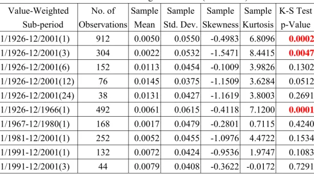
To estimate the RRA parameter β, we usemarket rate of return and riskless rate dataduring the period of December 1926 through December 2001. The summary statistics on the log month “Excess Return” on the value-weighted indexes (1926-2001) is presented in Table 1. And, the summary statistics on the log month “Excess Return” on the equal-weighted indexes (1926 - 2001) is presented in Table 2.

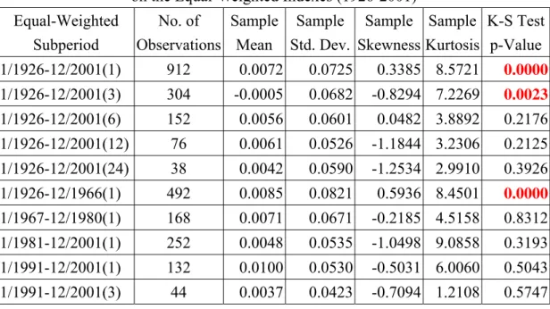
In both Tables 1 and 2, column 1 presents the subperiods while the number in the parentheses of each subperiod stands for the number of months. For example, in the first row of column 2, the number 912 represents for 912 monthly observations; in the fourth row of column 2, the number 76 stands for 76 annual observations; and finally, in the tenth row of column 2, the number of 44 stands for 44 tri-monthly observations. In both Table 1 and 2, Sample Mean, Sample Standard Deviation, Sample Skewness, and Sample Kurtosis are presented in column 3, 4, 5, and 6. Finally, the column 7 presents K-S Test Statistic for testing the normality of data in terms of different observation horizons.

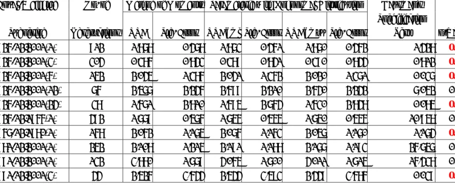
We have used two alternative methods – Parametric with Lognormal Distribution Method and Method of Moments, to estimate the relative risk aversion parameter β. The results are presented in Table 3 and Table 4, respectively. The data in Table 3 are estimated in terms of value-weighted indexes and in Table 4 are estimated in terms of equal-weighted indexes. In columns 1 and 2 in both Tables 3 and 4 are identical to column 1 and 2 in both Tables 1 and 2. Estimated RRA parameters in terms of Method of Moments and Parametric with Lognormal Distribution Method presented in columns 3 and 5, respectively.

F. Summary

In this project, we first briefly discussed the RRA estimation methods. Then, we use monthly market rate of return and riskless rate data to do the empirical study. The validity of the lognormal distribution for the excess market rate of return are also examined and tested before the RRA parameters are estimated. We use both the Parametric with Lognormal Distribution Method and the Method of Moments to estimate RRA parameters.

Table 1. Summary Statistics on the Log Month “Excess Return” on the Value-Weighted Indexes (1926-2001)

Value-Weighted No. of Sample Sample Sample Sample K-S Test Sub-period Observations Mean Std. Dev. Skewness Kurtosis p-Value 1/1926-12/2001(1) 912 0.0050 0.0550 -0.4983 6.8096 0.0002 1/1926-12/2001(3) 304 0.0022 0.0532 -1.5471 8.4415 0.0047 1/1926-12/2001(6) 152 0.0113 0.0454 -0.1009 3.9826 0.1302 1/1926-12/2001(12) 76 0.0145 0.0375 -1.1509 3.6284 0.0512 1/1926-12/2001(24) 38 0.0131 0.0427 -1.1619 3.8003 0.2691 1/1926-12/1966(1) 492 0.0061 0.0615 -0.4118 7.1200 0.0001 1/1967-12/1980(1) 168 0.0017 0.0479 -0.2801 0.7115 0.4240 1/1981-12/2001(1) 252 0.0052 0.0455 -1.0976 4.4722 0.1534 1/1991-12/2001(1) 132 0.0072 0.0424 -0.9536 1.9747 0.1083 1/1991-12/2001(3) 44 0.0079 0.0408 -0.3622 -0.0172 0.7291

Table 2. Summary Statistics on the Log Month “Excess Return” on the Equal-Weighted Indexes (1926-2001)

Equal-Weighted No. of Sample Sample Sample Sample K-S Test Subperiod Observations Mean Std. Dev. Skewness Kurtosis p-Value 1/1926-12/2001(1) 912 0.0072 0.0725 0.3385 8.5721 0.0000 1/1926-12/2001(3) 304 -0.0005 0.0682 -0.8294 7.2269 0.0023 1/1926-12/2001(6) 152 0.0056 0.0601 0.0482 3.8892 0.2176 1/1926-12/2001(12) 76 0.0061 0.0526 -1.1844 3.2306 0.2125 1/1926-12/2001(24) 38 0.0042 0.0590 -1.2534 2.9910 0.3926 1/1926-12/1966(1) 492 0.0085 0.0821 0.5936 8.4501 0.0000 1/1967-12/1980(1) 168 0.0071 0.0671 -0.2185 4.5158 0.8312 1/1981-12/2001(1) 252 0.0048 0.0535 -1.0498 9.0858 0.3193 1/1991-12/2001(1) 132 0.0100 0.0530 -0.5031 6.0060 0.5043 1/1991-12/2001(3) 44 0.0037 0.0423 -0.7094 1.2108 0.5747

Table 3 Estimation of Relative Risk Aversion on the Value-Weighted Indexes (1926-2001)

ue-Weighted No. of

Method of

Moments Parameteric with Lognormal Distribution Hausman's ubperiod Observations RRA Std. Error RRA_ml Std. Error RRA_mvu Std. Error

Specification Test p-Va 926-12/2001(1) 912 2.115 0.621 2.166 0.607 2.163 0.607 137.978 0. 926-12/2001(3) 304 1.264 1.088 1.291 1.080 1.286 1.084 12.778 0. 926-12/2001(6) 152 5.767 2.059 5.990 1.895 5.918 1.910 11.657 0. 926-12/2001(12) 76 8.872 3.726 10.839 3.489 10.563 3.554 171.964 0. 926-12/2001(24) 38 6.655 4.359 7.688 4.144 7.299 4.297 22.181 0. 926-12/1966(1) 492 2.062 0.762 2.110 0.741 2.103 0.742 35.914 0. 967-12/1980(1) 168 1.248 1.618 1.248 1.613 1.239 1.623 0.000 1. 981-12/2001(1) 252 2.881 1.440 3.039 1.404 3.018 1.410 61.444 0. 991-12/2001(1) 132 4.224 2.148 4.508 2.111 4.447 2.129 67.562 0. 991-12/2001(3) 44 5.173 3.855 5.221 3.830 5.001 3.936 0.528 0.

Table 4 Estimation of Relative Risk Aversion on the Equal-Weighted Indexes (1926-2001)

Equal-Weighted No. of Method of Moments Parameteric with Lognormal Distribution Hausman's Subperiod Observations RRA Std. Error RRA_ml Std. Error RRA_mvu Std. Error

Specification Test p-Va 926-12/2001(1) 912 1.878 0.478 1.873 0.461 1.870 0.462 1.428 0.2 926-12/2001(3) 304 0.386 0.843 0.389 0.841 0.390 0.844 0.812 0.3 926-12/2001(6) 152 2.045 1.386 2.041 1.362 2.020 1.371 0.037 0.8 926-12/2001(12) 76 2.577 2.246 2.699 2.210 2.640 2.242 7.052 0.0 926-12/2001(24) 38 1.671 2.810 1.695 2.764 1.630 2.848 0.085 0.7 926-12/1966(1) 492 1.779 0.576 1.756 0.555 1.750 0.556 10.958 0.0 967-12/1980(1) 168 2.062 1.175 2.076 1.163 2.057 1.170 1.174 0.2 981-12/2001(1) 252 2.108 1.215 2.191 1.188 2.177 1.193 26.757 0.0 991-12/2001(1) 132 3.880 1.779 4.065 1.700 4.011 1.715 16.438 0.0 991-12/2001(3) 44 2.526 3.644 2.544 3.593 2.449 3.686 0.039

References

1. Box, G. E. P., and D. R. Cox, “An analysis of transformations,” Journal of the Royal Statistical Society. Series B (Methodological), Vol. 26, No. 2. (1964), pp. 211-252. 2. Brown, D. P., and M. R. Gibbons, “A simple econometric approach for utility-based

asset pricing model,” Journal of Finance, Vol. 40, No. 2, June 1985, pp. 359 –381. 3. Casella, G., and George, E. I., “Explaining the Gibbs sampler,” American Statistician,

Vol. 46, 1992, pp. 167- 174.

4. Gelfand, A. E., and A. F. M. Smith, “Sampling-based approaches to calculating marginal densities,” Journal of American Statistics Association, Vol. 85, 1990, pp. 398 –409.

5. Gilks, W. R., S. Richardson, and Spiegelhalter, D. J., “Markov chain Monte Carlo in practice,” 1996, Campman and Hall, London.

6. Karson, M., D. Cheng, and Lee, C., “Sampling distribution of the relative risk aversion estimator: theory and applications,” Review of Quantitative Finance and Accounting, Vol. 5, No.1, March 1995, pp. 43 – 54.

7. Ljung, G. M., and G. E. P. Box, “Analysis of variance with autocorrelated observations,” Scan. Journal of Statistics, Vol. 7, 1980, pp. 172 – 180.

Part B: Alternative Hedge Ratio Estimates: Theory and Empirical Results

1. Introduction

One of the best uses of derivative securities such as futures contracts is in hedging. In the past, both academicians and practitioners have shown great interest in the issue of hedging with futures. This is evident from a large number of articles written in this area.

One of the main theoretical issues in hedging involves the determination of the optimal hedge ratio. However, the optimal hedge ratio depends on the particular objective function to be optimized. Many different objective functions are currently being used. For example, one of the most widely used hedging strategies is based on the minimization of the variance of the hedged portfolio (e.g., see Johnson, 1960; Ederington, 1979; and Myers and Thompson, 1989). This so-called minimum-variance (MV) hedge ratio is simple to understand and estimate. However, the MV hedge ratio completely ignores the expected return of the hedged portfolio. Therefore, this strategy is, in general, inconsistent with the mean-variance framework unless the individuals are infinitely risk-averse or the futures price follows a pure martingale process (i.e., expected futures price change is zero).

Other strategies that incorporate both the expected return and risk (variance) of the hedged portfolio have been recently proposed (e.g., see Howard and D'Antonio, 1984; Cecchetti, Cumby and Figlewski, 1988; and Hsin, Kuo and Lee, 1994). These strategies are consistent with the mean-variance framework. However, it can be shown that if the futures price follows a pure martingale process, the optimal mean-variance hedge ratio will be the same as the MV hedge ratio.

Another aspect of the mean-variance based strategies is that even though they are improvement over the MV strategy, for them to be consistent with the expected utility maximization principle, either the utility function needs to be quadratic or the returns should be jointly normal. If neither of these assumptions is valid, the hedge ratio may not be optimal with respect to the expected utility maximization principle. Some researchers have solved this problem by deriving the optimal hedge ratio based on maximization of the expected utility (e.g., see Cecchetti et al. (1988) and Lence (1995 and 1996)). However, this approach requires the use of specific utility function and specific return distribution.

Some attempts have been made to eliminate these specific assumptions regarding the utility function and return distributions. Some of them involve the minimization of mean extended-Gini (MEG) coefficient, which are consistent with the concept of stochastic dominance (e.g., see Cheung, Kwan and Yip, 1990; Kolb and Okunev, 1992 and 1993; Lien and Luo, 1993a; Shalit, 1995; and Lien and Shaffer, 1999). Shalit (1995) has shown that if the prices are normally distributed, the MEG based hedge ratio will be the same as the MV hedge ratio.

Recently, hedge ratios based on the generalized semivariance (GSV) or lower partial moments have been proposed (e.g., see De Jong, De Roon and Veld, 1997; Lien and Tse, 1998

and 2000; and Chen, Lee and Shrestha, 2001). These hedge ratios are also consistent with the concept of stochastic dominance. Furthermore, these GSV based hedge ratios have another attractive feature that they measure portfolio risk by the GSV, which is consistent with the risk perceived by managers because of its emphasis on the returns below the target return (see Crum, Laughhunn and Payne, 1981; and Lien and Tse, 2000). Lien and Tse (1998) have shown that if the futures and spot returns are jointly normally distributed and if the futures price follows a pure martingale process, the minimum-GSV hedge ratio will be equal to the MV hedge ratio.

Most of the studies mentioned above (except Lence (1995 & 1996)), ignore transaction costs as well as investments in other securities. Lence (1995 & 1996) derives the optimal hedge ratio where transaction costs and investments in other securities are incorporated in the model. Using a CARA utility function, Lence finds that under certain circumstances the optimal hedge ratio is zero, i.e., the optimal hedging strategy is not to hedge at all.

In addition to the use of different objective functions in the derivation of the optimal hedge ratio, previous studies also differ in terms of the dynamic nature of the hedge ratio. For example, some studies assume that the hedge ratio is constant over time. Consequently, these static hedge ratios are estimated using unconditional probability distributions (e.g., see Ederington, 1979; Howard and D'Antonio, 1984; Benet 1992; Kolb and Okunev, 1992 and 1993; and Ghosh, 1993). On the other hand, several studies allow the hedge ratio to change over time. In some cases, these dynamic hedge ratios are estimated using conditional distributions associated with models such as ARCH and GARCH (e.g., see Cecchetti et al., 1988; Baillie and Myers, 1991; Kroner and Sultan, 1993; and Sephton, 1993a). Alternatively, the hedge ratios can be made dynamic by considering a multi-period model where the hedge ratios are allowed to vary for different periods. This is the method used by Lien and Luo (1993b).

When it comes to estimating the hedge ratios, many different techniques are currently being employed. These techniques range from simple to complex ones. For example, some of them use such simple method as ordinary least squares (OLS) technique (e.g., see Ederington, 1979; Malliaris and Urrutia, 1991; and Benet, 1992). However, others use more complex methods such as the conditional heteroscadestic (ARCH or GARCH) method (e.g., see Cecchetti et al., 1988; Baillie and Myers, 1991; and Sephton, 1993a), the random coefficient method (e.g., see Grammatikos and Saunders, 1983), the cointegration method (e.g., see Ghosh, 1993; Lien and Luo, 1993b; and Chou, Fan and Lee, 1996), and the cointegration-heteroscadestic method (e.g., see Kroner and Sultan, 1993).

From the above discussion, it is clear that there are several different ways of deriving and estimating hedge ratios. In this report, we review these different techniques and approaches, and examine their relations.

The report is divided into four sections. In Section 2, alternative theories for deriving the optimal hedge ratios are reviewed while some empirical results of hedge ratios are discussed in Section 3. The Section 4 concludes with a summary.

2. Alternative Theories for Deriving the Optimal Hedge Ratio

The basic concept of hedging is to combine investment in the spots and futures to form a portfolio that will eliminate (or reduce) fluctuations in its value. Specifically, consider a portfolio consisting of C_s units long spot position and C_f units short futures position.1 Let

and denote the spot and futures prices at time t, respectively. Since the futures contracts are used to reduce the fluctuations in spot positions, the resulting portfolio is known as the hedged portfolio. The return on the hedged portfolio, , is given by:

t S F_t h R f s t s f t f s t s h R hR S C R F C R S C R = − = − , (1a) where t s t f S C F C

h= is the so-called hedge ratio, and

t t t s S S S R = +1− _and t t t f F F F R = +1− _are so-called one-period returns on the spot and futures positions, respectively. Sometimes, the hedge ratio is discussed in terms of price changes (profits) instead of returns. In this case, the profit on the hedged portfolio, ∆V_H, and the hedge ratio, H, are, respectively, given by:

∆V_H =C_s∆S_t−C_f∆F_t and s f C C = H , (1b) where ∆S_t =S_t+1−S_t and ∆F_t =F_t+1−F_t.

The main objective of hedging is to choose the optimal hedge ratio (either h or H). As mentioned above, the optimal hedge ratio will depend on a particular objective function to be optimized. Furthermore, the hedge ratio can be static or dynamic. In subsections A and B, we will discuss the static hedge ratio and then the dynamic hedge ratio.

It is important to note that in the above setup, the cash position is assumed to be fixed and we only look for the optimum futures position. Most of the hedging literature assumes that the cash position is fixed. This setup is suitable for financial futures. However, when we are dealing with commodity futures, the initial cash position becomes an important decision variable that is tied to the production decision. One such setup considered by Lence (1995, 1996) will be discussed in subsection C.

A. Static Case

In this section, we will discuss the following three alternative hedge ratios: A.1. Minimum-Variance Hedge Ratio

The most widely used static hedge ratio is the minimum-variance (MV) hedge ratio. Johnson (1960) derives this hedge ratio by minimizing the portfolio risk, where the risk is given by the variance of changes in the value of the hedged portfolio as follows:

(

V

)

C Var

( )

S C Var

( )

F C C Cov

(

S F Var ∆ _H = _s2 ∆ + 2_f ∆ −2 _{s f} ∆ ,∆

)

_. The MV hedge ratio, in this case, is given by:

(

)

( )

F Var F S Cov C C H s f J _∆ ∆ ∆ = = , * _{. (2a)}

Alternatively, if we use definition (1a) and use to represent the portfolio risk, the MV hedge ratio is obtained by minimizing which is given by:

(

Rh

Var

)

)

(

Rh

Var

( )

Rh Var

( )

Rs h Var

( )

Rf hCov

(

Rs Rf

)

Var _{= +} 2 ₋2 , _.

In this case, the MV hedge ratio is given by:

(

_{( )}

)

f s f f s J R Var R R Cov h σ σ ρ = = , * _{, (2b)}

where is the correlation coefficient between and , and and are standard deviations of and , respectively. The attractive features of the MV hedge ratio are that it is easy to understand and simple to compute. However, in general, the MV hedge ratio is not consistent with the mean-variance framework since it ignores the expected return on the hedged portfolio. For the MV hedge ratio to be consistent with the mean-variance framework either the investors need to be infinitely risk-averse or the expected return on the futures contract needs to be zero.

ρ R_s R_f σ_s σ_f

s

R R_f

A.2. Optimum Mean-Variance Hedge Ratio

Various studies have incorporated both risk and return in the derivation of hedge ratio. For example, Hsin et al. (1994) derive the optimal hedge ratio that maximizes the following utility function:

( )

(

)

( )

2 h h h C V E R A E R 05A Max f σ σ; . , = − , (3)

where A represents the risk aversion parameter. It is clear that this utility function incorporates both risk and return. Therefore, the hedge ratio based on this utility function would be consistent with the mean-variance framework. The optimal number of futures contract and the optimal hedge ratio are, respectively, given by:

( )

        − − = − = f s f f s f A R E S C F C σ σ ρ σ2 * 2 h . (4)

One problem associated with this type of hedge ratio is that in order to derive the optimum hedge ratio, we need to know the individual's risk aversion parameter. Furthermore, different individuals will choose different optimal hedge ratio, depending on the values of their risk aversion parameter.

Since the MV hedge ratio is easy to understand and simple to compute, it will be interesting and useful to know under what condition the above hedge ratio would be the same as the MV hedge ratio. It can be seen from equations (2b) and (4) that if or

, would be equal to the MV hedge ratio . The first condition is simply a restatement of the infinitely risk-averse individuals. However, the second condition does not impose any condition on the risk-averseness, and it is important. It implies that even if the individuals are not infinitely risk averse, the MV hedge ratio would be the same as the optimal mean-variance hedge ratio if the expected return on the futures contract is zero (i.e. futures prices follow a simple martingale process). Therefore, if futures prices follow a simple martingale process, we do not need to know the risk aversion parameter of the investor to find the optimal hedge ratio.

A→ ∞

( )

E R_f = 0 h₂ *

J

h

A.3. Sharpe Hedge Ratio

Another way of incorporating the portfolio return in the hedging strategy is to use the risk-return tradeoff (Sharpe measure) criteria. Howard and D'Antonio (1984) consider the optimal level of futures contracts by maximizing the ratio of portfolio excess return to its volatility:

( )

_, h F h C R R E Max f σ θ = − (5)

where and represents the risk-free interest rate. In this case, the optimal number of futures position, , is given by:

(

h h2 =Var R σ

)

R_F C*_f

( )

( )

( )

( )

__            − −         −       −               − = F s f f s F s f f s f s s f R R E R E R R E R E F S C C ρ σ σ ρ σ σ σ σ 1 * _{. (6)}

From the optimal futures position, we can obtain the following optimal hedge ratio:

( )

( )

( )

( )

__            − −         −       −         − = F s f f s F s f f s f s R R E R E R R E R E h ρ σ σ ρ σ σ σ σ 1 3 . (7)

Again, if E R

( )

_f = 0 h, ₃ reduces to: ρ σ σ         = s 3 h , (8)

which is the same as the MV hedge ratio . As pointed out by Chen et al. (2001), the Sharpe ratio is a highly nonlinear function of the hedge ratio. Therefore, it is possible that equation (7), which is derived by equating the first derivative to zero, may lead to the hedge ratio that would minimize, instead of maximizing, the Sharpe ratio. This would be true if the second derivative of the Sharpe ratio with respect to the hedge ratio is positive instead of negative. Furthermore, it is possible that the optimal hedge ratio may be undefined as in the case encountered by Chen et al. (2001), where the Sharpe ratio monotonically increases with the hedge ratio.

*

J

h

3. Some Empirical Results of Hedge Ratios

In this section, we will demonstrate how three alternative hedge ratios described in equations (2b), (4), and (7). To do the empirical work, we collect daily S&P index spot, S&P index futures, foreign exchange spot of British Pound, Deutsche Mark, and Japanese Yen, and foreign exchange futures of British Pound, Deutsche Mark, and Japanese Yen. The sample periods of this data are described in column 2 of Table 1.

Hedge ratio estimate in terms of Equations (2b) and (7) are presented in Table 1. In Table 1, hedge ratios are classified into (i) daily hedge ratio, (ii) weekly hedge ratio, and (iii) monthly hedge ratio. The estimated inputs: E(Rs), E(Rf),

σ

s,

τ

f, and

ρ

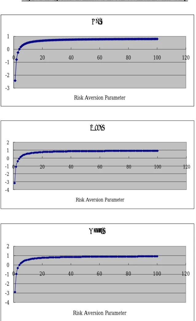
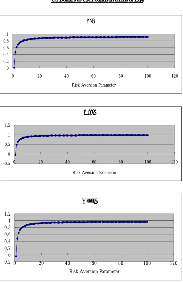
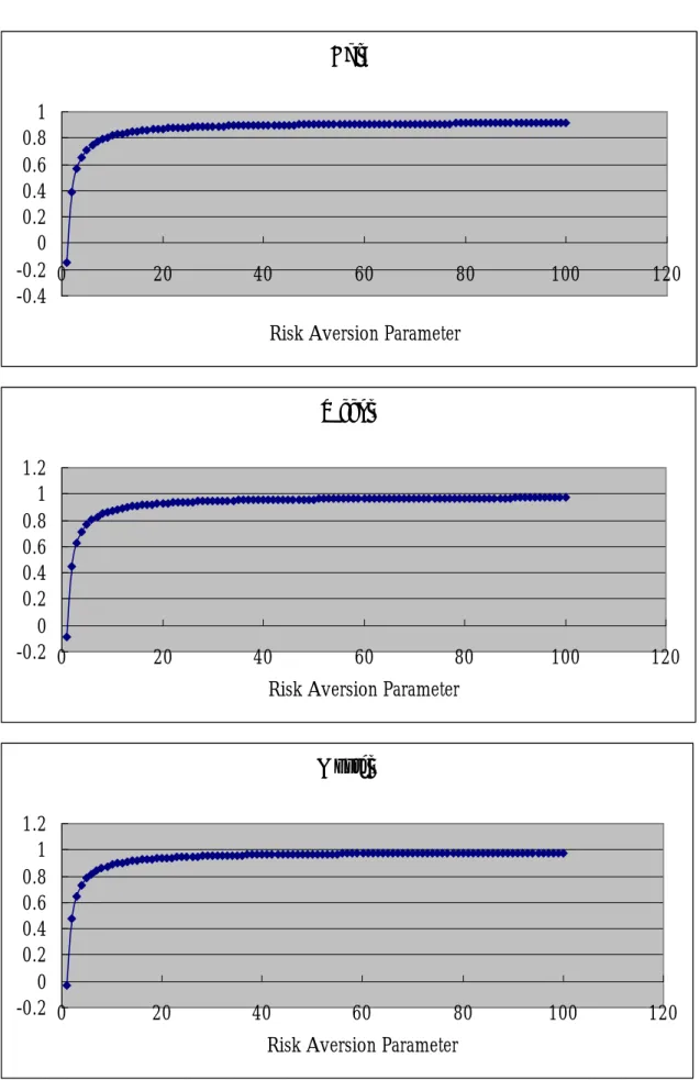
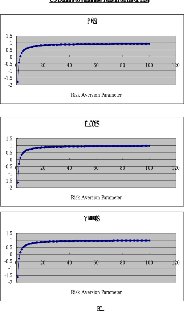
needed to estimate hedge ratio in terms of Equation (7) are presented in Table 2.

Figure 1 presents hedge ratio estimates of S&P500 index in terms of Equation (4). Figure 2 presents hedge ratio estimates of the foreign exchange rates of US Dollar to UK Pound in terms of Equation (4). Figure 3 presents hedge ratio estimates of the foreign exchange rates of US Dollar to Deutsche Mark in terms of Equation (4). And, Figure 4 presents hedge ratio estimates of the foreign exchange rates of US Dollar to Japanese Yen in terms of Equation (4). 4. Summary

In this report of the project, we have first review the literatures related to hedge ratio theories and estimation methods. Then, we have collected necessary data of S&P500 index, exchange rates of US Dollar to UK Pound, exchange rates of US Dollar to Deutsche Mark, and exchange rates of US Dollar to Japanese Yen to estimate hedge ratios in terms of three alternative methods. These three methods are (i) minimum-variance hedge ratio method, (ii) optimum mean-variance hedge ratio method, and (iii) Sharpe hedge ratio method.

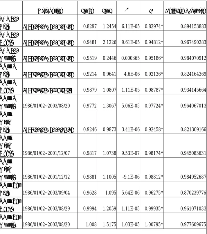
Table 1 Hedge Ratio Estimates in terms of Equations (2b) and (7)

Data Period Eq 2b Eq 7 Adjusted R-Square

S&P 500 Daily 1982/06/01~2003/09/04 0.8297 1.2454 6.11E-05 0.82974* 0.894153883 S&P 500 Weekly 1982/06/01~2003/09/04 0.9481 2.1226 9.61E-05 0.94812* 0.967490283 S&P 500 Monthly 1982/06/01~2003/09/04 0.9519 0.2446 0.000365 0.95186* 0.984070912 US to UK Daily 1986/01/02~2003/09/04 0.9214 0.9641 4.6E-06 0.92136* 0.824164369 US to UK Weekly 1986/01/02~2003/08/29 0.9879 1.0807 1.11E-05 0.98787* 0.934145664 US to UK Monthly 1986/01/02~2003/08/20 0.9772 1.3067 5.06E-05 0.97724* 0.964067013 US to Mark Daily 1986/01/02~2001/12/14 0.9246 0.9873 3.41E-06 0.92458* 0.821309166 US to Mark Weekly 1986/01/02~2001/12/07 0.9817 1.0738 9.53E-07 0.98174* 0.945083631 US to Mark Monthly 1986/01/02~2001/12/12 0.9881 1.1005 -9.1E-06 0.98812* 0.984952687 US to Yen Daily 1986/01/02~2003/09/04 0.9628 1.095 5.64E-06 0.96275* 0.870239776 US to Yen Weekly 1986/01/02~2003/08/29 0.9994 1.2059 1.11E-05 0.99935* 0.961071033 US to Yen Monthly 1986/01/02~2003/08/20 1.008 1.5175 1.03E-05 1.00795* 0.977609675 *無風險利率為 0.0155% *代表在 5%的顯著水準下拒絕參數為 0 的虛無假設 α _β

Table 2: Inputs for Estimating Hedge Ratio in terms of Equation (7) 現貨報酬率 平均值 [E(Rs)] 期貨報酬率 平均值 [E(Rf)] 現貨報酬率 標準差 (

σ

s) 期貨報酬率 標準差 (

τ

f) 報酬率 相關係數 (

ρ)

S&P 500 Daily 0.000457109 0.000477325 0.010635 0.01212 0.945607 S&P 500 Weekly 0.002256921 0.00227909 0.02267 0.023519 0.983626 S&P 500 Monthly 0.010054992 0.010180161 0.049349 0.051432 0.992035 US to UK

Daily 3.72134E-05 3.5395E-05 0.00632 0.006227 0.907856

US to UK

Weekly 0.000202561 0.000193806 0.013931 0.01363 0.966549 US to UK

Monthly 0.000996628 0.000968094 0.030738 0.030886 0.981957 US to Mark

Daily 5.05892E-05 5.10328E-05 0.007038 0.006899 0.906285 US to Mark Weekly 0.000249158 0.00025282 0.015507 0.015356 0.972188 US to Mark Monthly 0.001216577 0.001240427 0.03466 0.034814 0.992488 US to Yen Daily 0.000142889 0.000142563 0.007425 0.007195 0.932882 US to Yen Weekly 0.000744107 0.000733485 0.016995 0.016672 0.980364 US to Yen Monthly 0.003211607 0.003176038 0.035419 0.034745 0.988796 無風險利率為0.0155%

Figure 1: Hedge Ratio Estimates of the S&P 500 Index in terms of Eq4 Daily -3 -2 -1 0 1 0 20 40 60 80 100 120

Risk Aversion Parameter

Weekly -4 -3 -2 -1 0 1 2 0 20 40 60 80 100 1

Risk Aversion Parameter

20 Monthly -4 -3 -2 -1 0 1 2 0 20 40 60 80 100 120

Figure 2: Hedge Ratio Estimates of the Foreign Exchange Rates of US Dollars to UK Pounds in terms of Eq4

Daily 0 0.2 0.4 0.6 0.8 1 0 20 40 60 80 100 1

Risk Aversion Parameter

20 Weekly -0.5 0 0.5 1 1.5 0 20 40 60 80 100 1

Risk Aversion Parameter

20 Monthly -0.2 0 0.2 0.4 0.6 0.8 1 1.2 0 20 40 60 80 100 120

Figure 3: Hedge Ratio Estimates of the Foreign Exchange Rates of US Dollars to Deutsche Marks in terms of Eq4

Daily -0.4 -0.2 0 0.2 0.4 0.6 0.8 1 0 20 40 60 80 100 120

Risk Aversion Parameter

Weekly -0.2 0 0.2 0.4 0.6 0.8 1 1.2 0 20 40 60 80 100 120

Risk Aversion Parameter

Monthly -0.2 0 0.2 0.4 0.6 0.8 1 1.2 0 20 40 60 80 100 120

Figure 4: Hedge Ratio Estimates of the Foreign Exchange Rates of US Dollars to Japanese Yens in terms of Eq4

Daily -2 -1.5 -1 -0.5 0 0.5 1 1.5 0 20 40 60 80 100 120

Risk Aversion Parameter

Weekly -2 -1.5 -1 -0.5 0 0.5 1 1.5 0 20 40 60 80 100 120

Risk Aversion Parameter

Monthly -2 -1.5 -1 -0.5 0 0.5 1 1.5 0 20 40 60 80 100 120

References

Baillie, R.T. and R.J. Myers, 1991, "Bivariate Garch Estimation of the Optimal Commodity Futures Hedge," Journal of Applied Econometrics 6, 109-124.

Bawa, V.S., 1978, “Safety-First, Stochastic Dominance, and Optimal Portfolio Choice,” Journal of Financial and Quantitative Analysis 13, 255-271.

Benet, B.A., 1992, "Hedge Period Length and Ex-Ante Futures Hedging Effectiveness: The Case of Foreign-Exchange Risk Cross Hedges," Journal of Futures Markets 12, 163-175.

Box, G. E. P., and D. R. Cox, 1964, “An analysis of transformations,” Journal of the Royal Statistical Society. Series B (Methodological), Vol. 26, No. 2, 211-252.

Casella, G., and George, E. I., 1992, “Explaining the Gibbs Sampler,” American Statistician, Vol. 46, 1992, 167- 174.

Cecchetti, S.G., R.E. Cumby and S. Figlewski, 1988, "Estimation of the Optimal Futures Hedge," Review of Economics and Statistics 70, 623-630.

Chen, S.S., C.F. Lee, and K. Shrestha, 2001, “On a Mean-Generalized Semivariance Approach to Determining the Hedge Ratio,” Journal of Futures Markets 21, 581-598.

Chen, S.S., C.F. Lee, and K. Shrestha, 1998, “Alternative Approaches to Hedge Ratio: Theory and Empirical Analysis,” The 1998 Financial Management Association Annual Meetings.

Cheung, C.S., C.C.Y. Kwan and P.C.Y. Yip, 1990, "The Hedging Effectiveness of Options and Futures: A Mean-Gini Approach," Journal of Futures Markets 10, 61-74.

Chou, W.L, K.K. Fan and C.F. Lee, 1996, "Hedging with the Nikkei Index Futures: The Conventional Model versus the Error Correction Model," Quarterly Review of Economics and Finance 36, 495-505.

Crum, R.L., D.L. Laughhunn and J.W. Payne, 1981, “Risk-Seeking Behavior and Its Implications for Financial Models,” Financial Management 10, 20-27.

D'Agostino, R.B., 1971, “An Omnibus Test of Normality for Moderate and Large Size Samples,” Biometrika 58, 341-348.

De Jong, A., F. De Roon and C. Veld, 1997, “Out-of-Sample Hedging Effectiveness of Currency Futures for Alternative Models and Hedging Strategies,” Journal of Futures Markets 17, 817-837.

Dickey, D.A. and W.A. Fuller, 1981, "Likelihood Ratio Statistics for Autoregressive Time Series with a Unit Root," Econometrica 49, 1057–1072.

Ederington, L.H., 1979, "The Hedging Performance of the New Futures Markets," Journal of Finance 34, 157-170.

Engle, R.F. and C.W. Granger, 1987, "Co-Integration and Error Correction: Representation, Estimation and Testing," Econometrica 55, 251–276.

Fishburn, P.C., 1977, “Mean-Risk Analysis with Risk Associated with Below-Target Returns,” American Economic Review 67, 116-126.

Marginal Densities,” Journal of American Statistics Association, Vol. 85, 1990, 398 –409.

Geppert, J.M., 1995, “A Statistical Model for the Relationship between Futures Contract Hedging Effectiveness and Investment Horizon Length,” Journal of Futures Markets 15, 507-536.

Ghosh, A., 1993, "Hedging with Stock Index Futures: Estimation and Forecasting with Error Correction Model," Journal of Futures Markets 13, 743-752.

Gilks, W. R., S. Richardson, and Spiegelhalter, D. J., 1996, “Markov Chain Monte Carlo in Practice,” Campman and Hall, London.

Grammatikos, T. and A. Saunders, 1983, "Stability and the Hedging Performance of Foreign Currency Futures," Journal of Futures Markets 3, 295-305.

Howard, C.T. and L.J. D'Antonio, 1984, "A Risk-Return Measure of Hedging Effectiveness," Journal of Financial and Quantitative Analysis 19, 101-112.

Hsin, C.W., J. Kuo and C.F. Lee, 1994, "A New Measure to Compare the Hedging Effectiveness of Foreign Currency Futures versus Options," Journal of Futures Markets 14, 685-707.

Hylleberg, S. and G.E. Mizon, 1989, “Cointegration and Error Correction Mechanisms,” Economic Journal 99, 113-125.

Jarque, C.M. and A.K. Bera, 1987, “A Test for Normality of Observations and Regression Residuals,” International Statistical Review 55, 163-172.

Johansen, S. and K. Juselius, 1990, "Maximum Likelihood Estimation and Inference on Cointegration–With Applications to the Demand for Money," Oxford Bulletin of Economics and Statistics 52, 169–210.

Johnson, L.L., 1960, "The Theory of Hedging and Speculation in Commodity Futures," Review of Economic Studies 27, 139-151.

Junkus, J.C. and C.F. Lee, 1985, "Use of Three Index Futures in Hedging Decisions," Journal of Futures Markets 5, 201-222.

Kolb, R.W. and J. Okunev, 1992, "An Empirical Evaluation of the Extended Mean-Gini Coefficient for Futures Hedging," Journal of Futures Markets 12, 177-186.

Kolb, R.W. and J. Okunev, 1993, "Utility Maximizing Hedge Ratios in the Extended Mean Gini Framework," Journal of Futures Markets 13, 597-609.

Kroner, K.F. and J. Sultan, 1993, "Time-Varying Distributions and Dynamic Hedging with Foreign Currency Futures," Journal of Financial and Quantitative Analysis 28, 535-551.

Lee, C.F., E.L. Bubnys and Y. Lin, 1987, “Stock Index Futures Hedge Ratios: Test on Horizon effects and Functional Form,” Advances in Futures and Options Research 2, 291-311. Lence, Sergio H., 1995, “The Economic Value of Minimum-Variance Hedges,” American

Journal of Agricultural Economics 77, 353-364.

Lence, 1996, “Relaxing the Assumptions of Minimum Variance Hedging,” Journal of Agriculturel and Resource Economics 21, 39-55.

Lien, D. and X. Luo, 1993a, "Estimating the Extended Mean-Gini Coefficient for Futures Hedging," Journal of Futures Markets 13, 665-676.

Lien, D. and X. Luo, 1993b, "Estimating Multiperiod Hedge Ratios in Cointegrated Markets," Journal of Futures Markets 13, 909-920.

Lien, D. and D.R. Shaffer, 1999, “A Note on Estimating the Minimum Extended Gini Hedge Ratio,” Journal of Futures Markets 19, 101-113.

Lien, D. and Y.K. Tse, 1998, “Hedging Time-Varying Downside Risk,” Journal of Futures Markets 18, 705-722.

Lien, D. and Y.K. Tse, 2000, “Hedging Downside Risk with Futures Contracts,” Applied Financial Economics 10, 163-170.

Ljung, G. M., and G. E. P. Box, 1980, “Analysis of Variance with Autocorrelated Observations,” Scan. Journal of Statistics, Vol. 7, 172 – 180.

Malliaris, A.G. and J.L. Urrutia, 1991, "The Impact of the Lengths of Estimation Periods and Hedging Horizons on the Effectiveness of a Hedge: Evidence from Foreign Currency Futures," Journal of Futures Markets 3, 271-289.

Myers, R.J. and S.R. Thompson, 1989, "Generalized Optimal Hedge Ratio Estimation," American Journal of Agricultural Economics 71, 858-868.

Osterwald-Lenum, M., 1992, "A Note with Quantiles of the Asymptotic Distribution of the Maximum Likelihood Cointegration Rank Test Statistics," Oxford Bulletin of Economics and Statistics 54, 461–471.

Phillips, P.C.B. and P. Perron, 1988, "Testing Unit Roots in Time Series Regression," Biometrica 75, 335–46.

Rutledge, D.J.S., 1972, "Hedgers' Demand for Futures Contracts: A Theoretical Framework with Applications to the United States Soybean Complex," Food Research Institute Studies 11: 237-256.

Sephton, P.S., 1993a, “Hedging Wheat and Canola at the Winnipeg Commodity Exchange," Applied Financial Economics 3, 67-72.

Sephton, P.S., 1993b, “Optimal Hedge Ratios at the Winnipeg Commodity Exchange," Canadian Journal of Economics 26, 175-193.

Shalit, H., 1995, "Mean-Gini Hedging in Futures Markets," Journal of Futures Markets 15, 617-635.

Stock, J.H. and M.W. Watson, 1988, “Testing for Common Trends,” Journal of the American Statistical Association 83, 1097-1107.

Working, H., 1953, "Hedging Reconsidered," Journal of Farm Economics 35: 544-561

III. 計畫成果自評

With the results of this research project, we’ll submit two high quality papers to top academic journals in either economics or finance for publication by December 31,

出席國際學術會議心得報告

I have gone to the U. S. on November 13, 2002 to jointly in charge of the 13th Annual Conference on Financial Economics and Accounting with Professors Lemma W. Senbet, Gurdin Bakshi, Oliver Kim, and Lawrence A. Gordon. The 13th Conference on Finance Economics and Accounting was held at the University of Maryland on November 15-16, 2002. The result was both exciting and outstanding. This conference has become one of the most prestigious academic conferences in finance and accounting nationally and internationally. See the attached program for the details of the two-day event.

The fifteen-member executive committee (alphabetically) coordinated the program are as follows: Walter G. Blacconiere, Indiana University; Lawrence Brown, Georgia State

University; Martin Gruber, New York University; D. Erich Hirst, University of Texas at Austin; Bikki Jaggi, Rutgers University; Frank C. Jen, SUNY at Buffalo; Jayant R. Kale, Georgia State University; E. Han Kim, University of Michigan; Oliver Kim, University of Maryland;

Cheng-few Lee (conference coordinator), Rutgers University; Joe Ogden, SUNY at Buffalo; Joshua Ronen, New York University; Ehud I. Ronn, University of Texas at Austin; Lemma W. Senbet, University of Maryland; and Charles A. Trizcinka, Indiana University.

The detailed program is as follows:

November 15, 2002

12:00 Noon – 1:30 p.m. Lunch and Check-in at Inn & Conference Center 2:00 p.m. – 3:30 p.m.

Finance

❧ Session I: Corporate Finance and Governance (1511 VMH) Chairperson: Kose John, New York University

1. Corporate Governance Convergence by Contract: Evidence from Cross-Border Mergers

Arturo Bris, Yale University Christos Cabolis, Yale University

2. Horses and Rabbits? Optimal Dynamic Capital Structure from Shareholder and Manager Perspectives

Allen Poteshman, University of Illinois Nengjiu Ju, University of Maryland

Robert Parrino, University of Texas-Austin Michael Weisbach, University of Illinois

3. Organizational Form and Product Market Competition: Are Focused Firms Weak Competitors?

Sheri Tice, Tulane University

Naveen Khanna, Michigan State University

1. Toni Whited, University of Iowa

2. Robert McDonald, Northwestern University 3. Gordon Phillips, University of Maryland Accounting

❧ Session I: Pro-forma Earnings and Other Voluntary Disclosure (1505 VMH) Chairperson: Joshua Ronen, New York University

1. Voluntary Disclosures, Information Asymmetry and Reg FD Stephen Brown, Emory University

Stephen Hillegeist, Northwestern University Kin Lo, University of British Columbia

2. Earnings Quality and Strategic Disclosure: An Empirical Examination of Pro

Forma Earnings

Carol Marquardt, New York University

Barbara Lougee, University of California, Irvine 3. Are Investors Misled by “Pro Forma” Earnings?

William Schwartz Jr., University of Arizona Bruce Johnson, University of Iowa

Session Discussant:

Bala Dharan, Rice University

3:30 p.m. – 3:45 p.m. Break (Grand Atrium, VMH) 3:30 p.m. – 5:30 p.m.

Finance

❧ Session II: Asset Pricing (1511 VMH)

Chairperson: Craig MacKinlay, University of Pennsylvania 1. Testing Portfolio Efficiency with Conditioning Information

Wayne Ferson, Boston College

Andrew Siegel, University of Washington

2. Market Myopia, Market Mania, or Market Efficiency? An Examination of

Stock and Bond Price Reactions to R&D Increases and Subsequent Performance

Allan Eberhart, Georgetown University Akhtar Siddique, Georgetown University William Maxwell, University of Arizona 3. Revenue Growth and Stock Returns

Narasimhan Jegadeesh, University of Illinois

4. Testing Behavioral Finance Theories Using Trends and Sequences in Financial

Performance

Richard Frankel, MIT Wesley Chan, MIT S.P. Kothari, MIT

Discussants:

1. Anthony Lynch, New York University 2. Guojun Wu, University of Michigan 3. Jonathan Lewellen, MIT

❧ Session II: Earnings Management (1505 VMH)

Chairperson: Walter Blacconiere, Indiana University

1. Managers’ Guidance of Analysts: International Evidence Lawrence Brown, Georgia State University

Huong Ngo Higgins, Worcester Polytechnic Institute

2. The Relation Between Incentives to Avoid Debt Covenant Default and Insider

Trading

Messod Beneish, Indiana University Eric Press, Temple University

Mark Vargus, University of Texas, Dallas

3. Using Large Changes in Asset Turnover as a Signal of Potential Earnings Management

Ivo Jansen, Georgetown University Teri Yohn, Georgetown University

Session Discussant:

David Burgstahler, University of Washington 6:30 p.m. – 7:30 p.m. Cocktail Reception

7:30 p.m. – 9:00 p.m. Dinner and Keynote Address

(Inn & Conference Center – Main Ballroom) Keynote Speaker: Michael J. Brennan, UCLA

November 16, 2002

8:00 a.m. – 8:30 a.m. Continental Breakfast (Grand Atrium, Van Munching Hall) 8:30 a.m. – 10:00 a.m.

Finance

❧ Session III: Contract Design and Financial Intermediation (1511 VMH) Chairperson: Anjan Thakor, University of Michigan

1. The Impact of Organizational Form on Information Collection and the Value of

the Firm

Eitan Goldman, University of North Carolina 2. Optimal Contracts for Teams of Money Managers

Pegaret Pichler, Boston College

3. Does the Source of Capital Affect Capital Structure?

Michael Faulkender, Washington University in St. Louis Mitchell Petersen, Northwestern University

Discussants:

1. Simi Kedia, Harvard University 2. Amar Gande, Vanderbilt University

3. Hamid Mehran, Federal Reserve Bank of New York Accounting

❧ Session III: The Role of Formal Models in Interpreting Empirical Evidence (1505 VMH)

Chairperson: Thomas Hemmer, University of Chicago 1. Accruals, Returns, and Earnings

Carolyn Levine, Carnegie Mellon University Michael Smith, Duke University

2. The Effects of True and Perceived Ability Qi Chen, Duke University

Wei Jiang, Columbia University

3. On the Not so Obvious Relation between Risk and Incentives in Principal-Agent-Relations

Thomas Hemmer, University of Chicago

Session Discussant:

Bharat Sarath, CUNY, Baruch College 10:00 a.m. – 10:15 a.m. Break (Grand Atrium, VMH) 10:15 a.m. – 11:45 a.m.

Finance

❧ Session IV: Market Microstructure (1511 VMH) Chairperson: Charles Trzcinka, Indiana University

1. Evidence on the Speed of Convergence to Market Efficiency Avanidhar Subrahmanyam, UCLA

Tarun Chordia, Emory University Richard Roll, UCLA

2. Liquidity of Emerging Markets

David Lesmond, Tulane University

3. Institutional Trading Costs on Nasdaq: Have They Been Decimated? Ingrid Werver, Ohio State University

Discussants:

1. Elizabeth Odders-White, University of Wisconsin - Madison 2. Patrick Sandas, University of Pennsylvania

3. Charles Cao, Pennsylvania State University Accounting

❧ Session IV: Analyst Forecasts of Earnings (1505 VMH) Chairperson: Lawrence Brown, Georgia State University

1. Who is Afraid of Reg FD? The Behavior and Performance of Sell-Side

Analysts Following the SEC’s Fair Disclosure Rules

Anup Agrawal, University of Alabama Sahiba Chadha, University of Alabama

2. Has Regulation Fair Disclosure Affected Financial Analysts’ Ability to

Forecast Earnings?

Partha Mohanram, New York University Shyam Sunder, New York University

3. Analysts’ Forecasts in “Good-News” and “Bad-News” Environments: Evidence of Differential Timing of Information Arrival

Pradyot Sen, University of Cincinnati

Session Discussant:

Eric Zitzewitz, Stanford University

12:00 – 1:30 p.m. Lunch (Grand Atrium, VMH)

Distinguished Speaker: Robert E. Verrecchia, The Wharton School 1:45 p.m. – 3:15 p.m.

Finance

❧ Session V: International Finance (1511 VMH)

Chairperson: Vojislav “Max” Maksimovic, University of Maryland

1. Institutions, Markets and Growth: A Theory of Comparative Corporate

Governance

Kose John, New York University Simi Kedia, Harvard University

2. Patterns of Industrial Development Revisited: The Role of Finance Rqymond Fisman, Columbia University

Inessa Love, The World Bank 3. The World Price of Earnigns Opacity

Utpal Bhattacharya, Indiana University

Discussants:

1. Sugato Bhattacharyya, University of Michigan 2. Reena Aggarwal, Georgetown University 3. Raj Aggarwal, Dartmouth College

Accounting

❧ Session V: Extending the Analysis of the Earnings Returns Relation (1505 VMH) Chairperson: Jeffery Abarbanell, University of North Carolina

1. Earnings Quality and Price Quality Ran Hoitash, Rutgers University Murgie Krishnan, Rutgers University

Srinivason Sankaraguruswamy, Georgetown University

2. Rational Exuberance: The Fundamentals of Pricing Firms, from Blue Chip

to “Dot-Com”

Mark Kamstra, Atlanta Federal Reserve Bank

3. Loss Reversals and Valuation

Peter Joos, MIT George Plesko, MIT

Session Discussant:

Sudhakar Balachandran, Columbia University 3:15 p.m. – 3:30 p.m. Break (Grand Atrium, VMH) 3:45 p.m. – 5:45 p.m.

❧ Session VI: Derivatives and Risk Management (1511 VMH) Chairperson: Ehud Ronn, University of Texas - Austin 1. Overconfidence and Speculative Bubbles

Wei Xiong, Princeton University Jose Scheinkman, Princeton University

2. Idiosyncratic Risk and Creative Destruction in Japan Yasushi Hamao, University of Southern California Jianping Mei, New York University

Yexiao Xu, University of Texas - Dallas

3. Fed Funds Rate Targeting, Monetary Regimes and the Term Structure of

Interbank Rates: Explaining the Predictability Smile

Vassil Donstantinov, University of Wyoming 4. Modeling Credit Risk and Partial Information

Yildiray Yildirim, Syracuse University Unut Cetin, Cornell University

Robert Jarrow, Cornell University Philip Protter, Cornell University

Discussants:

1. Michael Gallmayer, Carnegie Mellon University 2. Burton Hollifield, Carnegie Mellon University 3. David Chapman, University of Texas - Austin 4. Greg Duffee, University of California - Berkeley Accounting

❧ Session VI: International Accounting (1505 VMH) Chairperson: Larry Gordon, University of Maryland

1. (Non) Convergence in International Accrual Accounting: The Role of

Institutional Factors and Real Operating Effects

Peter Joos, MIT Peter Wysocki, MIT

2. Economic Consequences from Mandatory Adoption of IASB Standards in the

European Union

Joseph Comprix, Arizona State University Karl Muller, Pennsylvania State University Mary Stanford-Harris, Texas Christian University

3. Stock Exchange Disclosure and Market Liquidity: An Analysis of 50 International Exchanges

Carol Frost, Dartmouth College Elizabeth Gordon, Rutgers University Andrew Hayes, Ohio State University

Session Discussant:

Christian Leuz, University of Pennsylvania