新穎交錯耦合濾波器之開發設計與寬頻高階馬迅平衡非平衡轉換器合成設計

(1)

國立交通大學

電信工程研究所

博士論文

新穎交錯耦合濾波器之開發設計與寬頻高階馬

迅平衡非平衡轉換器合成設計

Development and Design of Novel Cross-Coupled

Filters and Exact Synthesis of New High-Order

Wideband Marchand Balun

研究生：呂哲慶 (Jhe-Ching Lu)

指導教授：張志揚 (Chi-Yang Chang)

(2)

新穎交錯耦合濾波器之開發設計與寬頻高階馬迅平衡非

平衡轉換器合成設計

Development and Design of Novel Cross-Coupled Filters

and Exact Synthesis of New High-Order Wideband

Marchand Balun

研究生：呂哲慶

Student:

Jhe-Ching

Lu

指導教授：張志揚 Advisor:

Dr.

Chi-Yang

Chang

國立交通大學

電信工程研究所

博士論文

A Dissertation

Submitted to Institute of Communication Engineering

College of Electrical and Computer Engineering

National Chiao Tung University

in Partial Fulfillment of the Requirements

for the Degree of Doctor of Philosophy

in

Communication Engineering

September 2009

(3)

新穎交錯耦合濾波器之開發設計與寬頻高階馬迅平衡非平

衡轉換器合成設計

研究生:呂哲慶指導教授:張志揚

國立交通大學電信工程研究所

摘要

本論文主要的研究方向分成兩大部分，分別為微波濾波器設計與馬迅平衡非 平衡轉換器設計。第一部分是研究運用四分之ㄧ波長步階阻抗共振腔設計高性能濾波器、如何快速設計交錯耦合濾波器、以及發展新穎耦合濾波器。文中介紹使用四分之ㄧ波長步階阻抗共振腔來實現具有源級與負載相耦合的四角互耦的濾波器響應，可以任意控制第二對傳輸零點的位置。一般而言絕大部分的設計都是使用耦合係數與外部品質因子來設計濾波器，一旦共振腔型式固定，所萃取的耦合係數只能使用在當時濾波器的中心頻率與當時的實體佈局方式，而且一旦傳輸零點位置改變，共振腔擺放的位置也要改變，重新建立耦合係數與外部品質因子，而且其初始設計離最佳化的廣義柴比雪夫響應相差太多，必須調整濾波器的次數太多，造成難以快速設計。本論文提出以傳統平行耦合線濾波器來達到具有交錯耦合的功能，好處是能夠有最佳的初始設計以及優越的傳輸零點位置的擺放。此外，文中也提出新穎耦合濾波器圖形，此濾波器提供了對稱型的實體佈局實現非對稱的濾波器響應，也克服了傳輸零點非常靠近帶通頻率所造成在平面實體佈局技術的困難度。

(4)

論文的第二部份敘述使用傳輸線元件的分佈式電路所組成的網路的合成方法。此合成方法可以預測所有頻率點響應，所使用到的理查變數(Richards variable)、傳輸線網路、理查理論(Richards theorem)、黑田恆等式以及傳輸線近似合成函數都有討論。此外，文中也會提出高階寬頻馬迅平衡非平衡阻抗轉換器的電路，以及如何準確合成具有柴比雪夫響應的馬迅平衡非平衡阻抗轉換器。此種新提出的高階馬迅電路適合寬頻響應。

(5)

Development and Design of Novel Cross-Coupled Filters and

Exact Synthesis of New High-Order Wideband Marchand

Balun

Student: Jhe-Ching Lu Advisor: Dr. Chi-Yang Chang

Institute of Communication Engineering

National Chiao Tung University

Abatract

The research topics in this dissertation are divided into two parts; one is microwave filter design, the other is Marchand Balun design. The first topic is to utilize quarter-wave stepped impedance resonator to design high performance filter, study how to quickly design cross-coupled filters, and develop novel coupling schemes. In this dissertation, quarter-wave stepped impedance resonators are utilized to realize quadruplet and canonical-form coupling schemes. The proposed filter is easy to apply and control the source-load cross coupling. General speaking, most of the filter designs are to use coupling coefficients and external quality factor to design cross-coupled filters. Once the physical layout of the resonator is decided, the extracted coupling coefficients can be only used at the center frequency. Furthermore, if one coupling coefficient in the coupling matrix changes sign for shifting the transmission zero from one side of the passband to the other, the physical layout must

(6)

be reconfigured. The initial design of cross-coupled filters based on segmentation method is not good enough, so tuning of filter performances must spend much time. This dissertation presents new cross-coupled filters based on a conventional parallel-coupled filter. The proposed filters have the advantages of the ability to locate a transmission zero on the lower or upper stopband and a good initial design. Additionally, the novel coupling schemes are presented to exhibit bisymmetric coupling matrix. The novel coupling schemes provide the implementations of symmetric layouts to realize asymmetric filter responses. Using the novel coupling schemes implementation of generalized Chebyshev filters with transmission zeros very close to the passband can be easily realized in planar technology.

The second topic is to describe the synthesis method of the networks which are composed of the distributed transmission line circuits. The synthesis method is exact at all frequencies. Richards variable, transmission line networks, Richards theorem, kuroda identities and transmission line approximating functions are discussed in detailed. In addition, high-order wideband Marchand baluns are presented in this dissertation and the exact synthesis of the proposed Marchand baluns with Chebyshev responses are introduced. The proposed high-order Marchand baluns are suitable to design wideband responses.

(7)

誌謝首先，我最要感謝的是從小養育我長大的奶奶，還常常記得小時候的我體弱多病，常常得半夜找醫生，都是奶奶與姑姑們陪伴照顧著，沒有奶奶，我今日要求取博士學位，幾乎是不可能的，也感謝我能成長在喜樹這個好風水的鄉村，感謝喜樹的一切。我要特別感謝張志揚教授的指導。張教授的開朗與耐心以及對專業知識的熟稔，對於研究工作的進展有莫大的助益，也特別感謝老師給予學生研究的自由度。另外我也要感謝口試委員陳俊雄、郭仁財、呂良鴻、鍾世忠、林根煌、張盛富以及林祐生教授，在這七位口試委員的協助建議下，使本論文更顯完善。也要感謝在我博一時在研究上有些不懂的地方，而能準確重點地點破我的疑問的廖竟谷博士，很高興能夠與廖博士討論一些濾波器上的問題。接下來要感謝的另一批人是我那些台南從小到大的朋友。回到台南，常常跟你們混在一起，還蠻好玩的蠻開心的，讓我可以消除壓力，對後來的研究也有幫助。也感謝電子所黃博士、廖博士在我經濟困難之時幫助我。總之要感謝的貴人相當多，謝謝你們。呂哲慶於交大民國九十八年九月

(8)

List of Table

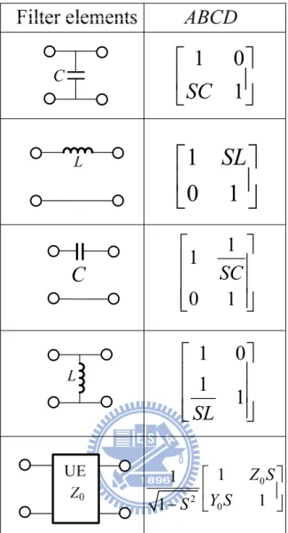
Table 2.1. Interesting well-known coupling topologies………...23 Table 2.2. ABCD matrices for distributed LC ladder and a unit element……….52 Table 4.1. The relative phase shifts of the main coupling path, the proper phases of the cross coupling paths to generate transmission zeros, corresponding responses, and delay line electrical length………73 Table 4.2. The physical dimensions of the two proposed filters………..84 Table 4.3. The dimensions of the first designed mixed cascaded quadruplet and

trisection filter with finite transmission zeros closed to the passband…….…………89 Table 6.1 The relationships between distributed circuits in the f-plane and high-pass circuits in the S-plane, and the corresponding ABCD parameters………..118

(11)

List of Figures

Fig. 1.1. Realization of an ideal balun by an ideal transformer………....9

Fig. 1.2. Marchand balun. (a) Type 1. (b) Type 2. (c) Type 3……….10

Fig. 1.3. Equivalent circuit of Marchand balun………...11

Fig. 1.4. Roberts balun (clipped from Fig. 3 in [103] )………...11

Fig. 1.5. Broadside-coupled balun (clipped from Fig. 2 in [111] )……….12

Fig. 1.6. A coupled-line Marchand balun………13

Fig. 2.1. Lowpass filter prototypes with ladder networks. (a) Begin with a shunt capacitor. (b) Begin with a series inductor………...18

Fig. 2.2. Alternative lowpass prototype networks using inverter. (a) K-inverters. (b) J-inverters……….18

Fig. 2.3. (a) Equivalent circuit of n-coupled resonators in low pass domain. (b) Its network representation……….19

Fig. 2.4. The coupling route of the example filter………...22

Fig. 2.5. A two-port network………...26

Fig. 2.6. Canonical transversal topology……….26

Fig. 2.7. A diagram shows that a 3-order transversal topology transforms into a wanted coupling topology………29

Fig. 2.8. Bandpass filters. (a) Use impedance inverters. (b) Use admittance inverters………31

Fig. 2.9. Generalized bandass filters. (a) K-inverters. (b) J-inverters……….31

Fig. 2.10. Inverters. (a) Lumped-element K inverters. (b) Lumped- and distributed -elements K inverters. (b) Lumped-element J inverters. (b) Lumped- and distributed-elements J inverters………33

Fig. 2.11. Pole-producing admittance inverters [57]……….34

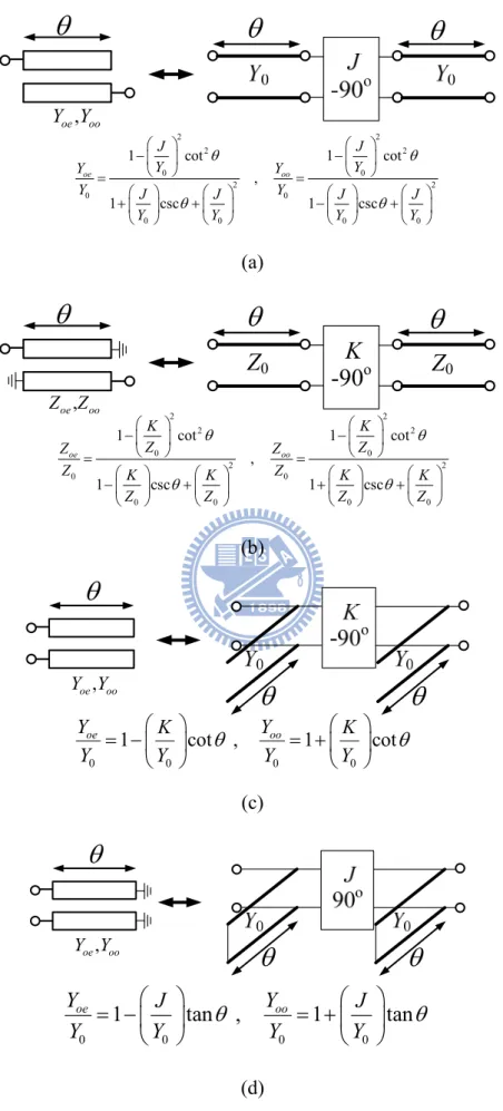
Fig. 2.12. Parallel- and antiparallel-coupled line circuits and its equivalent circuits… ………..35

Fig. 2.13. (a) Electrical coupling. (b) Magnetic coupling. (c) Mixed coupling……37

Fig. 2.14. Equivalent circuit of the I/O resonator with single loading………..39

Fig. 2.15. Typical coupling structures of coupled resonators. (a) Electric coupling. (b) Magnetic coupling. (c) and (d) Mixed coupling……….40

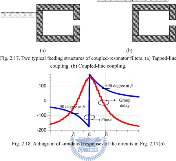
Fig. 2.16. A diagram of simulated responses of (a) electric coupling and (b) magnetic coupling………....40

Fig. 2.17. Two typical feeding structures of coupled-resonator filters. (a) Tapped-line line coupling. (b) Coupled-line coupling……….41

(12)

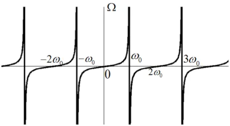
Fig. 2.19. Quarter-wavelength stepped impedance resonator type………...42 Fig. 2.20. A 2-order cross-coupled bandpass filter circuit………44 Fig. 2.21. Mapping between real frequency variableω and distributed frequency

variableΩ ………46

Fig. 2.22. Element transformation corresponding to the Richards transformation..46 Fig. 2.23. Richards transmission applied to an interconnecting transmission line...47 Fig. 2.24. A circuit used to illustrate the Richards theorem………..48 Fig. 2.25. The four Kuroda identities where 2

2 1

1

n = +Z Z ………...50

Fig. 2.26. (a) A high-pass prototype circuit. (b) A low-pass prototype circuit……..52 Fig. 3.1. The circuit layouts of the proposed microstrip quarter-wave SIR filters. (a)

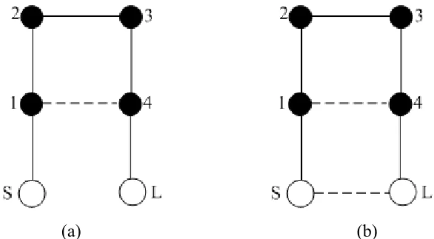
The fourth-order quadruplet filter. (b) The fourth-order quadruplet filter with source-load coupling………57 Fig. 3.2. Coupling schemes for the bandpass filters proposed in this dissertation. (a)

Quadruplet. (b) Canonical form………...58 Fig. 3.3. The basic structure of the quarter-wave SIR………59 Fig. 3.4. Basic coupling structures of the proposed filters. (a) The electric coupling.

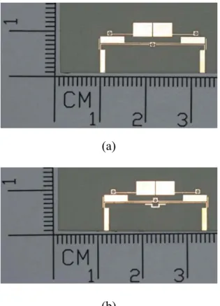
(b) The magnetic coupling. (c) The mixed coupling. (d) The coupled-line coupling for input/output coupling………..60 Fig. 3.5. The constructed filters. (a) The quadruplet filter. (b) The quadruplet filter

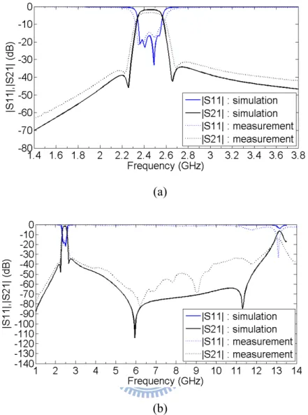
with source/load coupling………62 Fig. 3.6. Measured and simulated performances of the quadruplet filter of Fig.

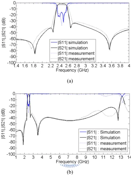
4.5(a). (a) In a narrow-band. (b) In a wide band………..63 Fig. 3.7. Measured and simulated performances of the quadruplet filter with source

/load coupling in Fig. 5(b). (a) In a narrow-band. (b) In a wide band….64 Fig. 4.1. The cross-coupled parallel coupled filter. (a) The schematic layout. (b)

Coupling and routing scheme corresponding to (a)……….69 Fig. 4.2. The equivalent lumped-element circuit of a fourth-order parallel coupled

filter……….70 Fig. 4.3. The cascaded trisection filter. (a) The coupling scheme. (b) The correspo-

nding equivalent lumped-element circuit of a fourth-order parallel coupled filter with cross couplings. Either the inverter JAD or JAE

corresponds to MS2 and either the inverter JJF or JJG corresponds to

M3L………74

Fig. 4.4. The mixed cascaded quadruplet and trisection filter. (a) The coupling scheme. (b) The corresponding equivalent lumped-element circuit of a fourth-order parallel coupled filter with cross coupling. Either the inverter

(13)

JAF or JAG corresponds to MS3 and either the inverter JJF or JJG

corresponds to M3L………...74

Fig. 4.5. The low-pass responses of the three CT filters with all in-band return loss 20dB. Case 1, normalized transmission zeros at Ω＝3 and Ω＝－2. Case 2, normalized transmission zeros at Ω＝3 and Ω＝2. Case 3, normalized transmission zeros at Ω＝－3 and Ω＝－2………..77 Fig. 4.6. The ideal responses of the two CQT filters. (a) The bandpass response

corresponding to (3.4) with a typical Chebyshev response as a reference. (b) The bandpass response corresponding to (3.5)………...80 Fig. 4.7. The circuit layouts of the proposed filters. (a) The first designed mixed

cascaded quadruplet and trisection filter. The length and line width of coupling/shielding line are 4.318 mm and 0.177 mm, respectively. (b) The second designed mixed cascaded quadruplet and trisection filter…81 Fig. 4.8. The layouts of the implemented filters. (a) The first designed filter. (b)

The second designed filter………83 Fig. 4.9. The measured and simulated performances of the two implemented filters. (a) The first designed filter. (b) The second designed filter……….86 Fig. 4.10. The sensitivity analysis of the first mixed cascade quadruplet and trisec-

tion filter for under etching of 0.0508 mm (2mil) and over etching of 0.0508 mm respectively………...86 Fig. 4.11. The simulated performances of the first mixed cascaded quadruplet and

trisection filter with finite transmission zeros at Ω=±1.4 , 4………88 Fig. 4.12. The simulated performances of the first mixed cascaded quadruplet and

trisection filter with finite transmission zeros at Ω=+1.5 , ±3………….90 Fig. 5.1. Cross coupling schemes generating transmission zeros at precise freque-

ncies. Conventional coupling schemes: (a) two-pole trisection. (b) three-pole cascade trisections (CQ). (c) three-pole quadruplet. Proposed coupling schemes: (d) two-pole interactive cross-coupling trisection scheme. (e) three-pole interactive cross-coupling quadruplet scheme. (f) four-pole interactive cross-coupling quadruplet scheme. (g) modified four-pole canonical form scheme with two pairs of transmission zeros. (h) modified three-pole cascade trisections (CT) scheme………..94 Fig. 5.2. (a) Parallel-coupled line section and (b) its equivalent circuit using a

J-inverter………104 Fig. 5.3. Ideal performances calculated from the synthesized coupling matrices in

(5.13) solid line, and (5.15) dotted line………..106 Fig. 5.4. The layouts and the simulated and measured performances of the filters in

(14)

Fig. 5.1(d). (a) Layout for the design with a transmission zero at Ω=3 (unit: mils). (b) Layout for the design with a transmission zero at Ω=-5 (unit: mils). (c) Simulated and measured results corresponding to Fig. 5.4(a). (d) Simulated and measured results corresponding to Fig. 5.4(b)………..107 Fig. 5.5. The proposed three-order CT filter. (a) Ideal real frequency responses. (b)

Layout (unit: mils). (c) Simulated and measured results………108 Fig. 5.6. The proposed third-order quadruplet filter. (a) Two ideal frequency responses: one is to consider the matrix in (5.19) solid line and the other is to exclude all the cross-coupling elements in (5.19) dotted line. (b) Layout (unit: mils). (c) Simulated and measured performances. (d) Layout for realizing the coupling scheme in Fig. 5.1(c)………..111 Fig. 5.7. The modified fourth-order quadruplet filter. (a) Ideal responses. (b) Lay-

out (unit: mils). (c) Simulated and measured performances…………...112 Fig. 5.8. The modified fourth-order quadruplet filter with source-load cross coupl-

ing. (a) Layout (unit: mils). (b) Simulated and measured performances………..113 Fig. 6.1. The distributed circuit of the proposed fifth-order Marchand balun…..116 Fig. 6.2. The proposed fifth-order Marchand balun. (a) The two-port distributed

circuit simplified in Fig. 6.1. (b) Its S-plane high-pass circuit………..117 Fig. 6.3. The first transformation. (a)The kuroda identity transformation from

[131]. (b) After kuroda identity transformation in Fig. 6.2(b)…..…….119 Fig. 6.4. The second transformation. (a) New exact circuit transformation. (b)

Apply exact circuit transformation in Fig. 6.4(a) to Fig. 6.3(b)………120 Fig. 6.5. The final fifth-order S-plane high-pass prototype of Marchand balun...120 Fig. 6.6. The ideal responses of the first and second designed baluns with bandwidth of 131% and 152%, respectively………125 Fig. 6.7. Physical layout of the first designed fifth-order balun with SC=j0.6 (unit:

mm)………126 Fig. 6.8. Measured and simulated performances of the first designed fifth-order

balun. (a) S₁₁ , S₂₁ and S₃₁ . (b) Amplitude balance and phase difference.

………126 Fig. 6.9. Physical layout of the second designed fifth-order balun with SC=j0.4

(unit: mm)………...127 Fig. 6.10. Measured and simulated performances of the second designed fifth-order

(15)

………128 Fig. 6.11. The sixth-order S-plane high-pass prototype of Marchand balun……...129

(16)

Chapter 1 Introduction

This dissertation includes two topics. The first topic is devoted to novel microwave cross-coupled filter design. The second topic is to design new higher-order Marchand balun based on exact synthesis technique.

1.1 Microwave Filters

Microwave filters are one of the important components in modern microwave communication systems. The frequency of microwave ranges from 300 MHz to 300 GHz corresponding to wavelengths (in free space) from 1 m to 1mm. The concept of electromagnetic waves should be used to describe the features of microwave components including microwave filters. Microwave filters are used to pass the wanted signals at frequencies within the passband and suppress the unwanted signals in the stopband. Filters for microwave applications must meet ever tighter specifications on electrical performances, and on size, weight, and reliability. The demands are growing more stringent on losses, steepness of cutoff, bandwidth, and linearity of phase shift (flat group delay). New features such as electronic tunability are being sought. Integrations of microwave filters with couplers, amplifiers, and frequency multipliers are becoming more important on system performance. To handle the rapid advance of applications of the modern communication systems, network analysis, accurate synthesis, design and diagnosis of filter networks have become one of the key technologies to fulfill the new challenges of reliability, insensitivity, low manufacturing cost, and minimum tuning effect on filter performance [1]-[2]. The historical review describing the development of the microwave filters is given in [3]-[5]. Different filter types and important references are given. Recently, among various kinds of microwave filters, microwave coupled-resonator filters are very popular. Generally, coupled-resonator filters with

(17)

cross coupling between nonadjacent resonators can exhibit steeper transfer function or flatter group delay, and they are called cross-coupled filters. The theory of cross-coupled filters [6], [7] provides a systematic design procedure that allows a filter with sharper selectivity and/or equalized group delay for various requirements in microwave systems. Most important characteristics of cross-coupled filters can be obtained by the corresponding coupling matrices.

1.1.1 Review of Coupled Resonator Filters and Cross-Coupled Filters

Initially, the research work on the design and synthesis of microwave filters can be traced back to the 1930’s [3]. At that time, network theory was probably the most advanced topic in engineering. The famous cascade synthesis theory as far back as 1939 [8] was published by S. Darlington. In his work, modern filter designs such as filters with finite frequency transmission zeros are included. The theory of direct-coupled cavity filters based on low-pass lumped-element prototype was presented by Fano and Lawson [3]. The main problem of Fano and Lawson theory was the lack of specific formulas for the low-pass prototype. The paper proposed by Cohn in [9] gives a comprehensive theory and extends the range of applicability to much broader bandwidths, i.e., about 20 percent in terms of guide wavelength. Later, in the 1960’s, a remarkable improvement in the applicable bandwidth to beyond 20 percent was made by Leo Young [10]. He succeeded in realizing the direct-coupled filters beyond 20 percent by using a distributed rather than a lumped-element prototype filter. In 1966, Levy [11] established a quite direct design in cavity filters and, thus enabling the desired parameters of the filter, i.e., number of cavities, ripple level, and band edges to be a simple formula which is used to derive the correct distributed prototype.

The first description of cross-coupled filters may be appeared to be by J. R. Pierce in the late 40’s [12]. However, the developments of cross-coupled filters took

(18)

place after 1965 or so. The cross coupling between nonadjacent resonators are introduced to generate transmission zeros. The cross coupling are mainly generated by the multipath. Applying suitable multi-path effect can bring transmission zeros from infinite to finite frequencies in the transfer function. Thus, attenuation poles at finite frequencies, or group delay flattening, or even both simultaneously can be achieved by observing the phases of the signals between different paths. A lot of related research works on the filter with cross coupling have been reported [12]-[33]. Furthermore, filter synthesis utilizing optimization techniques [34], [35] are used to obtain the required filtering functions.

Synthesis technique and implementation methods for the cross-coupled filters, which are shown in [12]-[35], have been developed for couples of decades. The most significant developments took place in the 1970’s in laboratories concerned with satellite communications, particularly at COMSAT by Atia and Williams [19]-[20], [23]. Their work on elliptic function and linear-phase waveguide filters using dual-mode cavities with cross coupling was particular significant. The dual-mode cavity filters introduced by Atia and Williams have resulted in the virtual standardization of these designs for satellite transponders.

Recently, one of the most important progresses in generalized filter synthesis is done by Richard Cameron. Richard Cameron published two papers [36], [37] which focused on generalizing the synthesis technique for the cross-coupled resonator filter with the generalized Chebyshev filtering function. With his work, N prescribed finite-position transmission zeros in an Nth-degree network are described. The synthesis method includes multiple input/output couplings, i.e., couplings may be made directly from the source and/or to load to internal resonators. The synthesized N+2 fully canonical coupling matrix for transversal array can completely describe all the possible generalized Chebyshev responses. With a series of similarity

(19)

transformations, the fully canonical coupling matrix can be reconfigured into a wanted coupling topology which is more convenient for the realization. The basic theory will be shown in Chapter 2.

Another attractive topic developed for several decades is the computer-aided diagnosis and tuning of cross-coupled filters. This is due to the continuous demand on reducing the manufacturing cost and development time for various filters with different specifications. It should be pointed out that filters with generalized Chebyshev responses are more difficult to fine tuned than that with Chebyshev or Butterworth responses. Thus, without a systematic adjustment method, it would spend much time on the tuning of filter performances, particularly for highly selective filters. Several research works focused on this problem [38]-[51]. The first effort for the adjustment and alignment of microwave filters can be traced back to Dishal [38] in the early 50’s when he utilized the filter return loss as the criterion for tuning. Atia and Williams [39] proposed a method for measurement of inter-resonator couplings based on measuring the phase responses of the reflection coefficient of a short-circuited network which consists of identical synchronously-tuned resonators. Thal [40] utilized the equivalent circuit in conjunction with phase measurement for filter diagnosis. In [41], a tuning method with short circuited networks for singly terminated filters is presented. In [42]-[44], different optimization strategies and schemes for parameter extraction are explored. Analytic methods in [45]-[47] are derived to extract the coupling matrix from the locations of system zeros and poles. In [48]-[50], the powerful Cauchy method is applied to get the rational polynomial approximation of reflection and transmission coefficients from the EM simulated results. In [51], eigenvalue approach is used to optimize the coupling matrix. The method in [52] utilized the Cauchy method in [48]-[50] to obtain the corresponding coupling matrix, and then optimize the rotation matrix to get the wanted coupling

(20)

topology. Besides, sensitivity of coupled resonator filters is analyzed in [53]. Thus, research concerning about cross-coupled filters have been studied for a long time, and up to present some researches are presenting.

1.1.2 Motivation

The requirements of highly selectivity, flat group delay, compact sizes, and wider rejection bandwidth are the significant studies of microwave filters. In addition, high reliability, low sensitivity, low manufacturing cost, and minimized fine-tuning steps on filter performance are also important.

Filters exhibiting high selectivity, broader upper stopband, and compact sizes are popular topics. Many published papers have achieved the requirements. However, the design method to control the finite transmission zeros is complex or difficult in most of the published papers. Furthermore, the layouts are usually too complicated for the published filters. To overcome the difficulties, a filter utilizing a 4-order canonical-form coupling scheme with λ/4 stepped impedance resonators may be a good choice.

In conventional cross-coupled filter designs, especially for microstrip filters, adjustment the distance and the orientation of each pair of neighboring resonators to get proper signs and magnitudes of the corresponding coupling coefficients is very tedious and time-consuming. The design curves of coupling coefficient and external Q for filters are generated from an electromagnetic (EM) field solver. Such filter designs can be found in Hong’s book [6]. When using this method as the initial dimensions of filters, filter designer has to spend much time to tune filter performances. To solve the drawbacks, new procedures to quick design of cross-coupled filters are demanded.

Another interesting topic is coupling schemes. The traditional 3-order trisection filter has one transmission zero on upper or lower stopband and the 4-order quadruplet filter has a pair of transmission zeros on both stopband. The order of the

(21)

advanced trisection and quadruplet can be two and three, respectively. However, there are problems of conventional or advanced trisection and quadruplet. As the transmission zero is close to the passband, serious asynchronously-tuned resonators for trisection cause serious effect on filter passband responses. Besides, when finite transmission zeros are very close to the passband, both trisection and quadruplet filters suffer from unrealizable gaps to implement the strong cross couplings. Thus, the solution of the problems may require new coupling schemes which can achieve trisection and quadruplet responses with transmission zeros close to the passband.

With the discussion described above, the first topic in this dissertation mainly focuses on different circuit design of filter with compact sizes, high selectivity and broad upper stopband, the development of new approach to cross-coupled filters, and novel coupling schemes with transmission zeros very close to passband.

1.1.3 Literature Survey of Coupling Schemes and Realizations of Cross-Coupled Resonator Filters

The existing well-known coupling schemes and the realizations of these coupling schemes are surveyed as follows.

In the past, numbers of research works concentrate on the coupling topologies of canonical form, cascade trisection (CT), and cascade quadruplet (CQ) [6], [24], [54]-[61]. Recently, the progressive development is to include source and load to nonadjacent resonator cross coupling [7], [52], [63]-[67]. The implementations of the three different coupling schemes were presented in [68]-[85]. In [70], the cross-coupling concept was firstly applied to the microstrip filters. Because of the increasing power of computations of computers, Hong and Lancaster introduced the method that by using electromagnetic (EM) simulators to get the S-parameters of the desired structure the cross-coupled resonator filters realized in microstrip line can be designed [70]-[72]. The coplanar waveguide structure is also presented to design

(22)

cross-coupled filters [83], [84]. Furthermore, broadside coupled coplanar stripline bandpass filters are designed to have finite transmission zeros successfully [85]. All the papers in [68]-[85] can use this method to design canonical form, cascade trisection, and cascade quadruplet filters with finite transmission zeros.

Recently, coupling schemes which exhibit so called zero-shifting properties were introduced and applied to waveguide resonator filters [66], [86], [87]. The main characteristic of the zero-shifting properties is the ability to shift a transmission zeros from one side of the passband to the other by adjusting the resonator frequencies of resonators instead of changing the sign of cross coupling. The doublet, extended doublet and box section with zero-shifting characteristic have been successfully implemented in microstrip form [88]-[90]. However, the coupling schemes are inherently sensitive due to the two main coupling paths.

As described above, it is worth studying new cross-coupled schemes and filter structures to solve these disadvantages.

1.1.4 Original Contribution of this Dissertation

The main contributions to cross-coupled filters in the first topic of this dissertation are addressed in three aspects.

First, a fourth-order canonical-form microstrip filter utilizing quarter-wave stepped-impedance resonators is presented. The requirements of compact sizes, sharp selectivity, and wide upper stopband for filters are achieved. The proposed circuit layout is easy to apply the source-load coupling and adjust the coupling strength.

Second, filters based on a conventional parallel-coupled structure [91]-[94] which exhibit generalized Chebyshev responses are proposed. The cross-coupled mechanisms of the proposed filters are originally investigated and presented. The observations of the two-port admittance matrix in the network can obtain the relative insertion phase from source or load to each open end of resonators. Thus, the cross

(23)

coupling can be applied using a delay line with proper electrical length. Due to the use of a conventional parallel-coupled structure, good initial dimensions can be obtained by the analytic method. Using the proposed structure, the conventional time-consuming adjusting procedure to obtain initial physical dimensions of filters, which is described in [6], is no longer required. Two fourth-order mixed cascade quadruplet and trisection filters are implemented to show properties of insensitive layout, flexible responses, good performance, and quick design procedures. With this approach, designer can eliminate tedious segmentation method for the filter design.

Finally, in this dissertation new coupling schemes where the corresponding coupling matrices show the bisymmetric property are proposed. Most of new coupling schemes have the properties of synchronous-tuned resonators, bisymmetric coupling matrices, and relatively weak cross-coupled strengths for finite transmission zeros very close to the passband. Filters with symmetrical layout are possible to implement the proposed bisymmetric coupling matrix that fine tuning of the filter would be much easier. Low-order planar filters with the proposed coupling schemes can achieve high selectivity.

1.2 Balun

In an unbalanced port, one of its two terminals is connected to the ground, an example being the output of a conventional signal generator. A balanced port, on the other hand, is one where both terminals are floating with respect to ground. Baluns are devices for interconnecting a balanced port to an unbalanced one. The ideal balun is a lossless, perfectly matched, two-port network whose properties are independent of frequency and power level, and may also provide impedance transformations as well. The ideal balun can be realized by the ideal transformer shown in Fig. 1.1, and deviations from the ideal depend solely on how closely one can realize the ideal transformer in practice.

(24)

Fig. 1.1. Realization of an ideal balun by an ideal transformer.

1.2.1 Literature Survey

Baluns (balanced-to-unbalanced) are important group of components which are used in circuits where a transition between unbalanced and balanced modes of excitation is required. The applications of baluns are frequently used in realizing balanced mixers, amplifiers, frequency multipliers, phase shifters, modulators, and dipole feeds, and numerous other applications. Over the past half-century, several different kinds of baluns [102]-[126] have been developed, and some research works on active baluns [127]-[129] are also attractive. In the course textbook [94], the contents of baluns and its applications may be good resources.

Among the various kinds of baluns, Marchand balun [102] is relatively popular because of its excellent amplitude and phase balance. Marchand’s famous paper [102] was published in December 1944. Marchand described three types of balun of increasing complexity and performance, which are shown in Fig. 1.2. The most sophisticated of the three types of baluns is shown in Fig. 1.2(c). The direct inspection of third type of balun can obtain the equivalent circuit shown in Fig. 1.3. To analyze and synthesize this balun the electrical lengths of the open and short-circuit stubs as well as the lengths of transmission lines must be the same, in which case the lengths of transmission lines are referred to as Unit Elements (U.E.) in filter technology. The description of Unit Elements will be discussed in Chapter 2.

(25)

4 λ (a) 4 λ 4 λ (b) Coaxial line Extended shield 4 λ Balanced two-wire line 4 λ Continuous shield Solid stub (c)

Fig. 1.2. Marchand balun. (a) Type 1. (b) Type 2. (c) Type 3.

shown in Fig. 1.4. Interestingly, the equivalent circuit of this coaxial balun is exactly the same as Marchand’s but the author made no reference to Marchand in his paper. However, the Roberts balun is a little easier to construct than Marchand’s.

(26)

Fig. 1.3. Equivalent circuit of Marchand balun.

Fig. 1.4. Roberts balun (clipped from Fig. 3 in [103] ).

Due to the equivalent circuit prototype shown in Fig. 1.3, the Marchand and Roberts balun are inherently band-pass networks. The simplest design techniques for these two baluns is to set Z1 and Z4 to the unbalanced and balanced port impedances,

respectively, and then the characteristic impedances of the two stubs can be designed from standard lumped element filter theory [6], [26]. The electrical lengths of the stubs and transmission lines are 90o at the center frequency of the balun. The responses of the baluns can be maximally flat (Butterworth) or equiripple (Tchebyshev) which depend on the values of the characteristic impedances.

In the 1980’s, two important papers proposed by Cloete [106], [107] showed graphs of the element values as a function of bandwidth and passband return loss of

(27)

Fig. 1.5. Broadside-coupled balun (clipped from Fig. 2 in [111] ).

the Marchand balun. Cloete designed a fourth-order Marchand balun with 15dB return loss over a decade bandwidth. The only limitation to use the design chart is that the balanced and the unbalanced ports can not have the same port resistance, but a 2:1 port resistance ratio. However, this is convenient if an anti-phase power divider is wanted instead of a balun since the 100 Ohms balanced load can be replaced by a 50 Ohm load connected between each of the balanced port’s terminals and ground.

There has been much interest in developing a planar structure of the Marchand or Roberts balun for use in monolithic and hybrid integrated circuits. One of the first papers to concern this issue is proposed by Pavio and Kikel [111]. The paper shows a whole view of the proposed structure, and this circuit is similar to Marchand balun. A broadside-coupled stripline structure is used to construct the balun, as shown in Fig. 1.5. The upper dielectric is very thin compared with the lower one, and, thus, considering coupling between the upper conductor and the ground plane could be ignored. So, the structure in Fig. 1.5 could be viewed as simply two transmission lines with upper and middle conductor forming one transmission line, and with the middle and lower conductor forming the other one. However, this structure is inherently a

(28)

Unbalanced port

Balanced port

Fig. 1.6. A coupled-line Marchand balun.

three-conductor coupled-line network, and detailed analysis of the structure must be taken into account.

Fig. 1.6 shows the coupled-line form of the edged-coupled planar Marchand balun. Several research works [115], [119], [120], [122], [125], [126] have focused on this edged-coupled version of Marchand balun. Goldsmith et al. [115] published the first comprehensive analysis of Fig. 1.6. The key point of analyzing coupled-line Marchand balun is that the two coupled-line sections have the same coupling coefficient. This results in the largely simplified design equations, which can be found in [119]. The design parameters derived by Goldsmith have successfully being connected to the coupling coefficient and even- and odd-mode impedances of the two coupled-line sections, which can be easy transformed into the physical parameters by using ADS or AWR circuit simulators. However, to design a balun having a decade bandwidth is not an easy task based on this coupled-line form of Marchand balun.

1.2.2 Objective and Contribution in the Second Topic of this Dissertation

The objectives of this balun research are to develop higher-order Marchand-type balun and to realize it in planar structure. With the proposed 5-order Marchand balun, a very wide bandwidth (152%) can be achieved, and the novel realization of the balun is to utilize microstrip line, slot line, and coplanar stripline. The 5-order Marchand baluns are synthesized by use of the Richard’s transformation and, thus, it means that the responses of the synthesized Marchand balun are exactly predicted at all

(29)

frequencies. Two examples of the 5-order Marchand balun are presented to demonstrate the design procedures. In addition, a 6-order Marchand balun is presented to discuss.

1.3 Organization of this Dissertation

This dissertation is organized as follows.

In Chapter 2, the first part is to introduce the basic theory of cross-coupled filters. The model of the cross-coupled filter in low-pass domain is given. The relation between a coupling matrix and S-parameter is derived from the model. Then, how to directly obtain the position of finite transmission zeros to a given coupling matrix is given. A conventional 3-order trisection is taken as an example. Some of interesting coupling schemes are arranged in a Table. A simple recursive formula to determine the generalized Chebyshev polynomials is given. Importantly, a general method for the synthesis of the coupling matrix in the transversal array is discussed. How to transform the coupling matrix from the transversal topology to the wanted coupling schemes by utilizing both eigenvalue approach and optimization is given. Lowpass prototype, generalized bandpass filters, impedance and admittance inverters, and the narrowband equivalence between coupled-line circuits and impedance and admittance inverters with transmission lines are introduced. Furthermore, coupled-resonator theory for extraction of external Q and coupling coefficients is given. To manipulate the spurious responses, the basic characteristics of stepped impedance resonators are discussed. How to obtain the relations between the coupling matrix and design parameters of coupled-resonator filters is presented. Those contents are useful in designing the cross-coupled filters which will be proposed in Chapter 3-5.

The second part in Chapter 2 is to consider distributed transmission line elements. To exactly synthesize the distributed transmission line networks, the Richards variable

(30)

and Richard theorem should be concerned and will also be discussed. The basic four Kuroda identities are given. General low- and high-pass S-plane prototype circuits are presented, and its corresponding characteristic functions are given. In addition, a synthesizing procedure is briefly discussed.

In chapter 3, two filters exhibiting quadruplet and canonical-form responses are designed. To extend the bandwidth of stopband, quarter-wave stepped impedance resonators are used. The use of the enhancing line of source-load coupling results in one additional pair of finite transmission zeros.

Chapter 4 describes microstrip parallel-coupled filters with generalized Chebyshev responses. The mechanism for generating finite transmission zeros is presented. The design procedures are discussed in detail. Two mixed cascade quadruplet and trisection filters are realized to demonstrate the feasibility. Furthermore, sensitivity analysis and a design guide to show the closest transmission zeros corresponding to realizable physical dimmensions are discussed by taking examples.

In chapter 5, new coupling schemes with the properties of bisymmetric coupling matrix, weak cross couplings, and synchronous-tuned or very tiny asynchronous-tuned resonators are presented. Bisymmetric coupling matrices imply symmetric layouts. The comparison between conventional and new proposed coupling schemes are discussed. The proposed bisymmetric coupling schemes can be used for the implementation of generalized Chebyshev filters with transmission zeros very close to the passband in planar technology.

Chapter 6 presents new higher-order Marchand balun with ultra wideband performances. Two network transformations, one is the Kuroda identity and the other is the proposed circuit transformation, are utilized to derive the final S-plane prototype circuit of Marchand balun. The exact synthesis and realization of the

(31)

proposed Marchand balun are discussed in detail.

(32)

Chapter 2 Theory of Microwave Resonator Filters and Distributed

Circuit Design

2.1 Basic Theory Used in Cross-Coupled Filters

In this section, the basic theory and design techniques for cross-coupled filters will be introduced. At first, the cross-coupled resonators network corresponding to the coupling matrix is analyzed in the normalized frequency domain. The relations between the normalized network parameters and S-parameters are derived. How to obtain the position of finite transmission zeros from coupling topologies is also given. In section 2.1.2, different types of impedance and admittance inverters are introduced, and the corresponding equivalent circuits are also presented. The frequently used coupled-line circuits and their equivalent circuits are provided. The segmentation method which is used to extract the external Q and the coupling coefficients is discussed in Section 2.1.3. Next, the characteristics of step impedance resonators will be reviewed. Finally, how to transform the synthesized coupling matrix to the design parameters of cross-coupled filters will be derived.

2.1.1 Synthesis Theory of Advanced Coupling Matrix in the Normalized Domain

The design of microwave filters normally starts from the synthesis of a low-pass prototype network which is shown in Fig. 2.1. Low-pass prototype networks are two-port network with an angular cutoff frequency of 1 rad/s and operating in a 1-Ω system. This type of lowpass filter can serve as a prototype for designing various practical filters with frequency and element transformations. The corresponding g values with different frequency responses, i.e. Butterwoth, Chebyshev, Elliptic function, and Gaussian responses, can be computed [6]. The alternative networks with impedance and admittance inverters as shown in Fig. 2.2 are also used. The networks in Fig. 2.2 can be represented by coupling matrices and are very useful for the design

(33)

Ω 1 Ω 1 (a) Ω 1 Ω 1 1Ω (b)

Fig. 2.1. Lowpass filter prototypes with ladder networks. (a) Begin with a shunt capacitor. (b) Begin with a series inductor.

Ω

1

1 Ω

(a)

Ω

1

1 Ω

(b)

Fig. 2.2. Alternative lowpass prototype networks using inverter. (a) K-inverters. (b) J-inverters.

of narrow band bandpass filter. So far, the cross coupling is not involved.

A general cross-coupled filter prototype of degree n in the lowpass domain is shown in Fig. 2.3 (a) [7], [90]. It is shown that this prototype can be obtained by

(34)

(a)

(b)

Fig. 2.3. (a) Equivalent circuit of n-coupled resonators in low pass domain. (b) Its network representation.

including all possible cross-coupling elements and frequency shifts of resonators. The prototype filter consists of frequency independent impedance inverters Ji,js, capacitors

Cis and susptances Bis. The values of all the capacitor and the terminated admittance

Y0 are set equal to one. The capacitors in the low-pass domain correspond to the

resonators in the bandpass domain. Thus, the frequency invariant susptance Bis

represent the frequency shift of resonators in the bandpass domain. The values of Bi

are zero for the synchronous filters and nonzero for the asynchronous filters. Applying circuit analysis of Kirchhoff’s current law to this prototype and stating the algebraic sum of the currents leaving a node in a network is zero, with a driving with a driving or external current of Is, the node equations for the circuit of Fig. 2.3(a) are shown in

(35)

1 ) 2 ( 1 ) 2 ( 1 1 0 ) 2 ( ) 2 ( 0 1 , 1 , 1 1 , 0 1 , 2 , 1 2 , 0 1 , 1 2 , 1 1 1 , 0 1 , 0 2 , 0 1 , 0 0 0 0 0 × + × + + + × + + + + + + + ⎥ ⎥ ⎥ ⎥ ⎥ ⎥ ⎦ ⎤ ⎢ ⎢ ⎢ ⎢ ⎢ ⎢ ⎣ ⎡ = ⎥ ⎥ ⎥ ⎥ ⎥ ⎥ ⎦ ⎤ ⎢ ⎢ ⎢ ⎢ ⎢ ⎢ ⎣ ⎡ ⎥ ⎥ ⎥ ⎥ ⎥ ⎥ ⎦ ⎤ ⎢ ⎢ ⎢ ⎢ ⎢ ⎢ ⎣ ⎡ + Ω + Ω n s n n n n n n n n n n n n n n I V V V V Y jJ jJ jJ jJ jB j jJ jJ jJ jJ jB j jJ jJ jJ jJ Y (2.1)

where Ω is the normalized frequency. The two-port S-parameters of a

coupled-resonator filter can be derived by the corresponding two-port network as shown in Fig. 2.3(b). Comparing Fig. 2.3(a) and Fig 2.3(b), one can find that V1=V0,

V2=Vn+1, and I1=Is-Y0V0. And 2 1 s I a = , 2 2 ₀ 1 s i V b = − 0 2 = a , b₂ =V_n₊₁ Thus, s a I V a b S 0 0 1 1 11 2 1 2 + − = = = (2.2) s n a I V a b S 1 0 1 2 21 2 2 + = = = (2.3) From (2.1), we can obtain

[ ]

1 1 , 1 0 _{= Y} − I V s (2.4)

[ ]

1 1 ), 2 ( 1 − + + ₌ n s n _Y I V (2.5) Substitute (2.4) into (2.2), one can obtain

1 1 , 1 11 1 2[ ] − + − = Y S (2.6) Substitute (2.5) into (2.3), thus enable obtaining

1 1 , 2 21 2[ ] − + = Y _n S (2.7) In the literatures, the matrix

(36)

⎥ ⎥ ⎥ ⎥ ⎥ ⎥ ⎦ ⎤ ⎢ ⎢ ⎢ ⎢ ⎢ ⎢ ⎣ ⎡ + + + + + + 0 0 1 , 1 , 1 1 , 0 1 , 2 , 1 2 , 0 1 , 1 2 , 1 1 1 , 0 1 , 0 2 , 0 1 , 0 n n n n n n n n n J J J J B J J J J B J J J J

is called the normalized coupling matrix and denoted as matrix [M].

⎥ ⎥ ⎥ ⎥ ⎥ ⎥ ⎦ ⎤ ⎢ ⎢ ⎢ ⎢ ⎢ ⎢ ⎣ ⎡ = 0 0 ] [ 1 12 2 1 12 11 1 2 1 nL L SL nL nn S L S SL S S M M M M M M M M M M M M M M M

where Mij=Ji,j, Mii=Bi. The admittance matrix is related to the normalized coupling

matrix, and can be expressed as

(

[ ] [ ] [ ]

)

[ ] ] [ ] [ ] [ ] [Y =s I + j M + G = j Ω U ₀+ M − j G = j A , where ][A]=Ω[U]₀+[M]− j[G , ( 2)( 2) 0]

[_U _∈_Rn+ ×n+ _{is identical to the identity}

matrix, except for the element [U₀]₁₁=[U₀]_n_{+ n}₂_, ₊₂ =0, and _[_G_]_∈_R(n+2)×(n+2)_{is also a}

diagonal matrix, [G]=diag{1,0, ,0,1}. The equations (2.6) and (2.7) can be rewritten as 1 1 , 1 11 1 2 [ ] − − − = j A S (2.8) S₂₁=−2 j

[ ]

A−₍_n1₊₂_),₁ (2.9) Similarly, one can derive

1 2 , 2 22 1 2 [ ] − + + − − = j A _n _n S (2.10)

The equations (2.8), (2.9) and (2.10) directly related the normalized coupling matrix to the S-parameters.

In the following, it will be shown that the position of finite transmission zeros can be predicted through transfer function. From the equations (2.8) and (2.9), one

(37)

can express S11 and S22 as rational functions, ) ( ) ( ) ( 11 _Ω Ω = Ω E F S (2.10) ) ( ) ( ) ( 21 _Ω Ω = Ω E P S (2.11) Obviously, the finite transmission zeros are the roots of the equation

P(Ω)=0 (2.12)

Solving the equation (2-12) can help to understand the dependence between the coupling coefficients and finite transmission zeros, thus enabling to get more insight to control the finite transmission zeros. An example to illustrate this procedure would be clear. Take a conventional 3-order trisection coupling scheme shown in Fig. 2.4 as an example.

Fig. 2.4. The coupling route of the example filter

The coupling matrix corresponds to the coupling topology of Fig. 2.4 is

1 1 11 12 13 12 22 23 13 23 33 3 3 0 0 0 0 0 0 0 0 0 0 0 0 S S L L M M M M M M M M M M M M M M ⎡ ⎤ ⎢ ⎥ ⎢ ⎥ ⎢ ⎥ = ⎢ ⎥ ⎢ ⎥ ⎢ ⎥ ⎣ ⎦ (2.13)

By solvingP(Ω)=0, one can find the roots, and it can be expressed as 12 23 22 13 Ω M M M M = − + (2-14) When −M₂₂+(M M₁₂ ₂₃ M₁₃) 0> , a transmission zero on upper stopband occurs.

(38)

1 2 S L 1 2 3 S L 1 2 3 S L 1 2 3 S L 1 2 3 4 S L 1 2 4 S L 3 1 2 4 S L 3 1 2 S L 2 1 S L 3 3 2 S 1 4 L 5 2 S 1 6 L 3 4 1 2 3 4 S L 5

2-order trisection 3-order trisection 3-order cascade trisection

3-order quadruplet 4-order quadruplet 4-order mixed cascade

quadruplet and trisection

4-order canonical form Doublet Extended doublet

Box section Cul-de-sac

5-order cascade quadruplet Coupling schemes

Table 2.1 Interesting well-known coupling topologies.

While −M₂₂+(M M₁₂ ₂₃ M₁₃) 0< , a transmission zero on lower stopband is created. Several interesting well-known coupling schemes [6], [7], [66], [67] are shown in Table 2.1.

From the discussion as described above, we know the cross-coupled filter exhibits finite transmission zeros (attenuation poles), which means the responses of cross-coupled filters may correspond to the generalized Chebyshev responses. In fact, how to generate the S₁₁(s) andS₂₁(s) corresponding to the generalized Chebyshev functions and find the corresponding coupling matrices are important and

(39)

well-established. Many synthesis methods for cross-coupled filters have been proposed in [20], [34]-[37]. In this dissertation, we adopted the simple recursion formula [34] proposed by Smain Amari to determine the low-pass prototype with generalized Chebyshev responses and focused on the transversal array method [37] proposed by Richard Cameron to obtain coupling matrices.

The reflection and transfer polynomials of cross-coupled filters with generalized Chebyshev responses can be obtained by using the recursion formula as follows. The transfer function S21(ω ) is '

( )

2

_{( )}

21 2 2 1 ' 1 _N ' S F ω ε ω = + (2.15)

where ω is the frequency variable in a low-pass prototype, ε is a constant related to ' the inbandreturn loss R which is

_ε ₌

[

₁₀R/10₋₁

]

−1/2_(2.16)

The characteristic filtering function FN(ω ) is '

( )

1

( )

1 ' 1 ' ' cosh cosh , 1 ' ' N n N n n n n F ω x x ω ω ω ω − = − ⎛ ⎞ = _⎜ _⎟ = − ⎝

∑

⎠ (2.17)

where, 's_n = jω _n is the location of the nth transmission zero in the low-pass normalized domain, and |FN(ω =±1)|=1 for all value of N. The function F' N(ω ) is a '

rational function, and it can be expressed as

( )

1 ( ') ( ') ' ( ') ' 1 ' N N N _N N n n P P F D ω ω ω ω ω ω = = = ⎛ ⎞ − ⎜ ⎟ ⎝ ⎠

∏

(2.18)

To compute PN(ω ) a simple recursion relation is established between P' N-1(ω ), '

PN( ω ) and P' N+1( ω ). Using the identity cosh(α±β)= cosh(α)cosh(β) '

∓ sinh(α)sinh(β), we can write

1 1 1 1 1 1 ( ')

cosh cosh ( ) cosh ( )

' 1 ' N N n N n N N P x x D ω ω ω − − + + = + ⎛ ⎞ = _⎜ + _⎟ ⎛ ⎞ _⎝ _⎠ − ⎜ ⎟ ⎝ ⎠

∑

(40)

1 1 1 1 1 1 1 1 1 1 1 1

sinh cosh ( ) sinh(cosh ( )) cosh( cosh ( ))

( ')

sinh cosh ( ) sinh(cosh ( ))

N N n N n N n n N N n N N n N x x x x P x x x D ω − − − + + = = − − + + = ⎛ ⎞ = _⎜ _⎟ + ⎝ ⎠ ⎛ ⎞ = _⎜ _⎟ + ⎝ ⎠

∑

(2.19) Similarly,

( )

(

( )

)

( )

1 1 1 1 ' 1 ' ' '

sinh cosh sinh cosh

N _N N N n N N n N N P P x x x D D ω _ω ω ω − − − = ⎛ ⎞ − ⎜ ⎟ ⎛ ⎞ ⎝ ⎠ _{= −} ₊ ⎜ ⎟ ⎝

∑

⎠ (2.20)

From equation (2.19) and (2.20), by using hyperbolic identities the recursion relation is obtained as the following equation.

( )

(

)

(

)

( )

(

)

(

)

1 2 2 2 1 1 1 ₂ 1 2 1 2 2 1 1 2 2 1 1 1 ' ' ' ' 1 ' _{1 1} _' 1 1 ' 1 1 ' ' ' ' ' _{1 1} _' N N N N _N N N N N _N P P P ω ω ω ω ω _ω ω ω ω ω ω ω _ω + + − + + − ⎛ ⎞ = − _⎜ − _⎟ ⎝ ⎠ − ⎡ _⎛ _⎞ ₋ ⎤ ⎢ ⎥ + − +_⎜ − _⎟ ⎢ _⎝ _⎠ ₋ ⎥ ⎣ ⎦ (2.21)

where the polynomials P0(ω')=1, P1(ω')=ω'-1/ω'₁. Thus, the transfer and reflection

polynomials for the generalized Chebyshev filtering function can be expressed in the form

( )

2 2 2 21 ' 2 2 2 2 N N N N N D D S D P E ω ε = = + , or 21

( )

' N N D S E ω = (2.22)

( )

2 2 2 2 2 11 ' 1 21 ' 2 2 N N N N N E D F S S E E ω = − ω = − = , or ₁₁

( )

' N N F S E ω = (2.23) The next step is to synthesize the coupling matrix.

When concerning the canonical transversal topology, considering admittance function is advantageous to synthesize this transversal coupling scheme. The first step is to construct the two-port short-circuit admittance parameter matrix [YN] for the

overall network. Fig. 2.5 shows a two-port network terminated in a 1 Ω resistance, and Fig. 2.6 is the canonical transversal topology.

Following the analytical formula in [37], one can get the transversal matrix having the following form

(41)

Fig. 2.5. A two-port network.

Fig. 2.6. Canonical transversal topology.

1 2 1 11 1 2 1

0

S S SL S L S nn Ln SL L Ln

M

⎡

⎤

⎢

⎥

⎢

⎥

⎢

⎥

=

⎢

⎥

⎢

⎥

⎢

⎥

⎣

⎦

(2.24)

(42)

Detailed derivation procedures can be found in [37]. Here, we only summarized important equations and design parameters of the transversal topology. First, the admittance function [YN] can be synthesized from the transfer and reflection

polynomials in (2.22) and (2.23). The numerator and denominator polynomials for the y21(s) and y22(s) elements of [YN] are built up directly from the transfer and reflection

polynomials for S21(s) and S11(s). Then, the following equation for the admittance

matrix [YN] for the overall network:

[ ]

11

( )

_{( )}

12

( )

_{( )}

0

₍

₎

11 12 1 21 22 0 21 22 0 1 0 N k k N k k k k y s y s K r r Y j y s y s K = s jλ r r ⎡ ⎤ ⎡ ⎤ ⎡ ⎤ =_⎢ _⎥= _⎢ _⎥+ ⋅_⎢ _⎥ − ⎣ ⎦ ⎣ ⎦ ⎣ ⎦

∑

(2.25)

Here, the residues r21k and r22k may be found from partial fraction expansions of the

denominator and numerator polynomials for y21(s) and y22(s), and the purely real

eigenvalues λk of the network found by rooting the denominator polynomial common

to both y21(s) and y22(s), which has purely imaginary roots = jλk.

Second, another two-port admittance matrix [YN] is to cascade the elements in

Fig. 2.6(c), thus gives an ABCD transfer matrix for the kth “low-pass resonator” as follows:

[

]

(

)

0 k k LK SK SK LK k SK LK sC jB M M M M ABCD M M ⎡ + ⎤ ⎢ ⎥ ⎢ ⎥ = − ⎢ ⎥ ⎢ ⎥ ⎢ ⎥ ⎣ ⎦ (2.26)

which can then be converted into the equivalent short-circuit y-parameter matrix

[ ]

(

)

2 2 1 _SK _SK _LK k k k SK LK LK M M M y sC jB M M M ⎡ ⎤ = _{⋅ ⎢} _⎥ + _⎣ _⎦ (2.27)

The admittance matrix [YN] for the parallel-connected transversal array is the sum of

the y-parameter matrices for the N individual sections, plus the y-parameters matrix [ySL] for the direct source-load coupling inverter MSL

(43)

[ ]

(

)

2 SL 2 1 SL 0 ₁ 0 N SK SK LK N k k k SK LK SK M M M M Y j M = sC jB M M M ⎡ ⎤ ⎡ ⎤ = _⎢ _⎥+ _{⋅ ⎢} _⎥ + ⎣ ⎦

∑

⎣ ⎦ (2.28)

Comparison of (2.25) and (2.28) shows

(

) (

)

(

) (

)

21 2 22 k SK LK k k k k LK k k k r M M s j sC jB r M s j sC jB λ λ = − + = − + (2.29)

Thus, by equating the real and imaginary parts in (2.29), important extracted circuit parameters are

(

)

2 22 21 1 k k kk k LK k SK LK k C B M M r M M r λ = ≡ = − = = (2.30)

The synthesis of the transversal topology is complete.

Although the coupling matrix of the transversal topology is so far synthesized, the transformations of coupling matrices from the transversal topology to the wanted coupling schemes are necessary due to the easy realization of coupling schemes. Fig. 2.7 shows a diagram describing what topologies is a 3-order transversal topology transformed into. In [37], it is difficult to determine the rotation angles of the sequence of similar transformation. So, the eigenvalue approach [51] to optimizing the coupling matrix of the wanted couping scheme is adopted in this dissertation. It is very powerful for extracting the coupling matrix of filters with order under 14. A briefly review of this method is discussed as follows.

The transversal coupling matrix (2.24) is denoted as

0 0 T S SL S L t T L SL r r M r r r r ⎡ ⎤ ⎢ ⎥ =_⎢ Λ _⎥ ⎢ ⎥ ⎣ ⎦ (2.31)

(44)

2 1 S L 3 Extended doublet 1 2 3 S L 3-order trisection 1 2 3 S L

3-order cascade trisection

1 2 3 S L 3-order quadruplet 2 1 S L 3

A 3-order transversal topology

Fig. 2.7. A diagram shows that a 3-order transversal topology transforms into a wanted coupling topology.

Let R denote the product of elementary plane rotations involving orthogonal rotations among the planes 1 to N

1 0 0 0 0 0 0 1 T T R X ⎡ ⎤ ⎢ ⎥ = ⎢ ⎥ ⎢ ⎥ ⎣ ⎦ (2.32)

where X is an orthogonal matrix, and 0 represents the zero vector. Applying similarity transformations to the matrix M_t one obtains desired coupling matrix M in the form

新穎交錯耦合濾波器之開發設計與寬頻高階馬迅平衡非平衡轉換器合成設計

國 立 交 通 大 學

電信工程研究所

博 士 論 文

新穎交錯耦合濾波器之開發設計與寬頻高階馬

迅平衡非平衡轉換器合成設計

Development and Design of Novel Cross-Coupled

Filters and Exact Synthesis of New High-Order

Wideband Marchand Balun

研 究 生：呂哲慶 (Jhe-Ching Lu)

指導教授：張志揚 (Chi-Yang Chang)

新穎交錯耦合濾波器之開發設計與寬頻高階馬迅平衡非

平衡轉換器合成設計

Development and Design of Novel Cross-Coupled Filters

and Exact Synthesis of New High-Order Wideband

Marchand Balun

研究生：呂哲慶

Student:

Jhe-Ching

Lu

指導教授：張志揚 Advisor:

Dr.

Chi-Yang

Chang

國立交通大學

電信工程研究所

博士論文

A Dissertation

Submitted to Institute of Communication Engineering

College of Electrical and Computer Engineering

National Chiao Tung University

in Partial Fulfillment of the Requirements

for the Degree of Doctor of Philosophy

in

Communication Engineering

September 2009

新穎交錯耦合濾波器之開發設計與寬頻高階馬迅平衡非平

衡轉換器合成設計

研究生:呂哲慶 指導教授:張志揚

國立交通大學電信工程研究所

摘要

Development and Design of Novel Cross-Coupled Filters and

Exact Synthesis of New High-Order Wideband Marchand

Balun

Student: Jhe-Ching Lu Advisor: Dr. Chi-Yang Chang

Institute of Communication Engineering

National Chiao Tung University

Abatract

Contents

List of Table

List of Figures

Chapter 1 Introduction

Chapter 2 Theory of Microwave Resonator Filters and Distributed

Circuit Design

Ω

1

1

Ω

Ω

1

1

Ω

[ ]

[ ]

(

)

[ ]

( )

( )

[

]

( )

( )

∑

( )

∏

∑

∑

∑

∑

國立交通大學

博士論文

研究生：呂哲慶 (Jhe-Ching Lu)

研究生:呂哲慶指導教授:張志揚

_{( )}

_{( )}

_{( )}

₍

₎