利用深度學習法於藥物不良反應信號偵測

(1)

國立高雄大學資訊工程學系

碩士論文

利用深度學習法於藥物不良反應信號偵測

Applying Deep Learning to Signal Detection of Adverse

Drug Reactions

研究生：王成浩撰

指導教授：林文揚博士

(2)

(3)

i

致謝

對於能夠順利的完成此篇論文，我特別感謝我的指導教授林文揚教授，是教授指引了我在這個過去從沒有深入過的人工智慧領域中探索、研究，期間不論我提出了多少問題、遭遇了多少困難，教授從來不吝於教導，從根本一步步的教會我，同時也訓練我，讓我在獨立研究、論文寫作、口頭報告上的能力有所增進。我也特別感謝兩位口試委員洪宗貝老師、蘇家輝老師，兩位老師都在口試時提出可貴的建議與修改的方向，讓我能從不同面向審視論文中的問題。接著，我也很感謝同一個實驗室的研究夥伴以及已經離開實驗室的學長姐，在研究的這段期間，除了研究上的互助上，生活上的交流也緩解了感受到的壓力。最後，我要感謝我的家人，他們總是在我的背後默默的支持著我，對於學習的需要總是二話不說地提供給我，讓我可以沒有後顧之憂的學習。

(4)

ii

利用深度學習法於藥物不良反應信號偵測

指導教授：林文揚博士（教授）國立高雄大學資訊工程學系學生：王成浩國立高雄大學資訊工程學系摘要藥物不良反應一直是醫療領域關注的議題，因為它會造成病人生理上、經濟上的嚴重負擔，因此許多國家紛紛建立了自發性通報系統(SRS)，例如：美國食品藥物管理局(FDA)的不良反應事件通報系統(FAERS)。過去幾年，有許多學者提出了基於統計方法的異常信號偵測方法，其缺點為缺乏學習的能力，沒有辦法透過舊有資料來學習。因此，我們嘗試使用深度學習方法利用FAERS 系統中的藥品的資訊來進行新上市藥品的不良反應信號偵測。由於，卷積神經網路在各個領域上都有卓越的表現，我們選擇使用卷積神經網路來建構不良反應信號偵測的模型。在 FAERS 的報告中所記載的藥物與不良反應之間的關係並沒有被驗證過，而卷積神經網路是一種端到端(end-to-end)的模型，輸入端與輸出端之間的關係必須要是正確的才能確保模型能夠正確運行。此外，真實狀況下藥物可能產生多種不良反應，對於端到端模型來說，在有無數種不良反應的狀況下，這會變成一個無法學習的多標籤(Multi-label)問題。如果把它轉換為單標籤問題，意即，只鎖定一種特定的不良反應，又會造成資料的嚴重不平衡，以及出現有樣本紀錄同樣藥物、但紀錄會產生及不會產生特定不良反應的狀況，我們將其稱為困惑的樣本。我們提出了一系列的方法來解決這些問題，我們通過 SIDER 資料庫來驗證藥物與不良反應之間的關係，並用SMOTE 方法解決了資料不平衡的問題。針對困惑的樣本，我們將記錄藥物不會產生特定不良反應的困惑樣本刪除。整體而言，我們提出了一個能夠將FAERS 的資料轉換為卷積神經網路所需的輸入形式的前置處理方法。我們鎖定了心肌梗塞這個危險又致命的不良反應，用 SIDER 驗證後的 FAERS 的資料訓練用來進行不良反應信號偵測的卷積神經網路，然後從 FDA 的不良反應事件安全報告中找到了7 種不在 SIDER 紀錄中，也就是未出現在訓練用的資料中的藥物，其角色如同新上市藥品。我們將這7 種藥物相關的紀錄做為測試集，並使用訓練好的模型來進行測試。實驗結果顯示，若考慮在MedDRA 中的HLT 層，我們的模型在 7 個測試集中偵測到的信號都較 FDA 的不良反應事件安全報告早，平均而言，要早16 季。

(5)

iii

關鍵字：藥物不良反應、自發性通報系統、FAERS 資料庫、信號偵測、深度學

(6)

iv

Applying Deep Learning to Signal Detection of Adverse

Drug Reactions

Advisor: Dr. (Professor) Wen-Yang Lin

Department of Computer Science and Information Engineering National University of Kaohsiung

Student: Cheng-Hao Wang

Department of Computer Science and Information Engineering National University of Kaohsiung

Abstract

Adverse drug reactions (ADR) have long been a concerned issue of medical and healthcare community because it will cause serious physiological and economic burdens on patients. Therefore, many countries have established Spontaneous Reporting Systems (SRS), such as FDA Adverse Event Reporting System (FAERS), which was established by the US Food and Drug Administration (FDA). Many scholars have proposed statistical-based methods to detect ADR signals, which however lack ability to learn from historical data. Therefore, we try to use deep learning methods to detect ADR signals of new marketing drugs through the data of FAERS. Since convolutional neural networks have performed well in various fields, we chose it to build a model for ADR signal detection.

However, the relationship between the drugs and adverse reactions recorded in the FAERS reports has not been verified. The convolutional neural network is an end-to-end model. The relationship between the input and the output must be correct to ensure that the model learns correctly. Moreover, drugs may cause a variety of adverse reactions. For end-to-end models, this will become an un-learnable multi-label problem in the presence of numerous adverse reactions. If we transferred the problem to a single-label problem which means only one specific adverse reaction is targeted, it will cause serious imbalance of data. It also causes a situation that there are samples recording the same drug but recording both the target and untarget adverse reactions, which we name it perplexing negatives. We proposed a series of methods to solve these problems. We verified the relationship between drugs and adverse reactions by the SIDER dataset. Then, we solved the problem of data imbalance by the SMOTE method. For the perplexing negatives, we eliminated the instances that record the drug but not cause the

(7)

v

adverse reaction. Overall, we propose a preprocessing procedure for transferring the FAERS data to the input that the convolutional neural network requires.

We focused on a dangerous and fatal adverse reaction, myocardial infarction. We used the SIDER-verified FAERS data to train a convolutional neural network for ADR signal detection. We found seven kinds of drugs that may cause myocardial infarction from FDA's safety report. These drugs are not listed in the SIDER, that is, the drugs are not in the training sets, so can be regarded as the newly marketed drugs. We use the instances that recorded these seven drugs as testing sets and detect them by our proposed CNN models. Our results show that if we consider adverse reactions in HLT level of MedDRA, the ADR signals our models detected in the seven test sets were earlier than the FDA's alerts, on average, 16 quarters ahead.

Keywords: Adverse drug reaction, signal detection, spontaneous reporting system,

(8)

vi

Content

Chapter 1 Introduction ... 1

1.1 Motivation ... 1 1.2 Contributions... 2 1.3 Thesis Organization ... 2

Chapter 2 Background Knowledge and Related Work ... 4

2.1 FDA Adverse Event Reporting System (FAERS) ... 4

2.2 ADR Detection ... 5

2.3 Deep Learning and CNN ... 8

2.4 Related Work ... 11

Chapter 3 The Proposed Deep Learning ADR Prediction

Framework ... 15

3.1 Preprocessing... 15

3.1.1 Class labeling ... 16

3.1.2 Class disambiguation ... 17

3.1.3 Class binarization ... 18

3.1.4 Class imbalance handling... 20

3.2 Model Building ... 22

3.2.1 Data transformation ... 22

3.2.2 Model structure ... 23

Chapter 4 Experimental Results ... 25

4.1 Experimental Design ... 25

4.2 Effect of Perplexing Negatives ... 26

4.3 Model Selection ... 27

4.4 Models Trained by SIDER Alone ... 29

4.5 Model Evaluation ... 31

Chapter 5 Conclusions and Future Work ... 62

(9)

vii

5.2 Future Work ... 63

(10)

1

Chapter 1 Introduction

1.1 Motivation

Patients have been plagued by adverse drug reactions (ADRs) for a long period of time. Adverse drug reactions can cause serious medical and economic burdens on patients, and sometimes even lead to death. Therefore, many countries have established spontaneous reporting systems (SRS) for the detection and analysis of adverse drug reactions [29]. The information gathered by these systems is provided to researchers for analysis to facilitate research related to adverse drug reactions. In the past few years, there have been many analytical methods such as proportional reporting ratio (PRR) [8], reporting odds ratio (ROR) [24], and chi-square [9], etc. However, these statistics-based methods lack the ability of learning from the rich features provided by the SRS data, such as patient demographics, and anatomical, therapeutics, and chemical information of drug coding. In light of the advancement of machine learning and its success in many applications, we endeavor to apply machine learning methods to the detection of ADRs using SRS data.

In recent years, deep learning has exhibited outstanding performances in many areas, such as image classification and segmentation. In fact, as long as we can extract the features of data, we can analyze different kinds of data through these features, not just images. Convolutional neural network (CNN) is a branch of deep learning, which has the ability to extract features. This motivates us to adopt CNN to extract automatically appropriate features from the reporting cases

(11)

2

of patients taking drugs with the help of some knowledge base of ADRs, such as SIDER [41] and drugbank [36], to establish a model for future ADR detection for newly marketing or pre-marketing drugs.

1.2 Contributions

The main contributions of this thesis are:

1. We proposed a preprocess that transfers FAERS data to a binary-class ADR dataset. The process resolves uncertain class labeling, perplexing negatives and class imbalancing problems.

2. We proposed a method that based on CNN to detect ADR signals. Unlike traditional statistics-based methods, our deep learning based model can learn from the rich data and features in the FAERS database.

3. We conducted experiments to validate the usability of our proposed model. The results show our model can detect all testing ADR signals far before FDA’s alerts. In the HLT level of MedDRA [39], our best models can detect the signals, on average, 16 quarters ahead of FDA’s warning.

1.3 Thesis Organization

The rest of this thesis is organized as follows.

Chapter 2 presents some background knowledge related to this work and summarized state-of-the-art drug-related research. Section 2.1 describes FAERS, the most well-known spontaneous reporting system. Section 2.2 describes some existing methods for detecting adverse drug reactions. Section 2.3 introduces what is deep learning and shows the structure of the convolutional neural network. Section 2.4 summarizes some related work.

(12)

3

Chapter 3 presents the complete process and framework of our CNN-based ADR detection method. Section 3.1 elaborates the preprocess of transferring the FAERS data into a training set meets the CNN model. Section 3.2 describes how we input data into models and the structure of CNN-based model.

Chapter 4 presents our experiments and results. Section 4.1 describes the experimental environment and the data we used. In Section 4.2, we present the experiment to examine the effect of perplexing negatives. In Section 4.3, we show different models and their results on different test sets. Section 4.4 describes how to decide the structure of the model through experiments. Section 4.5 presents the performance results of our proposed model on ADR detection.

(13)

4

Chapter 2 Background Knowledge and Related Work

In this chapter, we will present some background knowledge of our study, including FAERS system, ADR detection methods, deep learning, and related work.

2.1 FDA Adverse Event Reporting System (FAERS)

FAERS [37] is a system designed to support FDA’s post-marketing safety surveillance program for drug and therapeutic biologic products. This system receives adverse event reports, medication error reports and product quality complaints that resulting in adverse events directly from healthcare professionals and consumers.

The data collected by FAERS are released to the public every quarter since 2004. The data schema is composed of seven related tables as organized in Table 2.1.

Table 2.1 Table summary of FAERS database

Table Name Content

Demo Record demographic information such as patient's age, weight, gender, etc., and administrative information such as the time and result of the event.

Drug Record detailed information about the drug, including the name of the drug, the dose, the route, etc.

Reac Record adverse reactions, coded in terms of preferred term in MedDRA [39].

Outc Record patient outcome codes for the event. RPSR Record reporting source code for the event.

THER For each drug in each event, record the drug therapy start dates and end dates.

INDI Record indications, coded in terms of preferred term in MedDRA.

(14)

5

On average, more than 100,000 reports were collected quarterly in FAERS. There are some limitations on the usage of FAERS. For example, the casual relationship between a drug and an adverse reaction is uncertain and the reports may not contain enough information to show all the factors of an adverse events.

2.2 ADR Detection

ADR detection refers to the task for measuring the causality relationship between a drug and an adverse reaction (from spontaneous reporting system data such as FAERS) so as to identify potential ADR signals (pairs of drugs and reactions) for further evaluation.

In the literature, there have been many ADR detection methods. Most of them are statistic-based approaches and can be classified into two categories: simple disproportionality and Bayesian methods. Both require counting the number of occurrences of patterns represented in a contingency table shown as Table 2.2, where a represents the number of cases that symptom S occurs after taking drug D, b represents the number of cases that other symptoms S occurs after taking drug D, c represents the number of cases that symptom S occurs after taking other drug D, and d represents the number of cases that other symptoms S occurs after taking other drugs D.

Table 2.2 Contingency table for ADR detection

Symptom S Others Symptom S Total

Drug D a b a+b

Others Drugs D c d c+d

(15)

6

Typical disproportionality measurements include Proportional Reporting Ratio (PRR), Reporting Odds Ratio (ROR), chi-square (χ2_{), RR [23], and IC [14]. Definitions} of these measurements are summarized in Table 2.3.

Table 2.3 Formula of typical disproportionality measures.

Measure Formula PRR 𝑎𝑎/(𝑎𝑎 + 𝑏𝑏) 𝑐𝑐/(𝑐𝑐 + 𝑑𝑑) ROR 𝑎𝑎/𝑏𝑏 𝑐𝑐/𝑑𝑑 χ2 χ2 ₌ _� (|χ − E(χ) − 12|) 2 𝐸𝐸(χ) χ∈{𝑎𝑎,𝑏𝑏,𝑐𝑐,𝑑𝑑}

E(n) : Expect value of n.

RR 𝑎𝑎(𝑎𝑎 + 𝑏𝑏 + 𝑐𝑐 + 𝑑𝑑)

(𝑎𝑎 + 𝑏𝑏)(𝑎𝑎 + 𝑐𝑐) IC

𝑙𝑙𝑙𝑙𝑙𝑙2𝑎𝑎/(𝑎𝑎 + 𝑏𝑏 + 𝑐𝑐 + 𝑑𝑑)_{(𝑎𝑎 + 𝑏𝑏)/(𝑎𝑎 + 𝑐𝑐)}

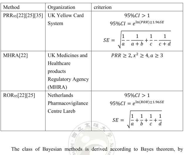
The class of simple disproportionality methods compute one or several ones of the measures to determine whether a drug-ADR pair is a potential signal for further inspection. Examples include the PRR hybrid method used by EU and UK, the ROR method by the Netherlands Pharmacovigilance Foundation, which are summarized in Table 2.4.

(16)

7

Table 2.4 A summary of prevailing disproportionality methods Method Organization criterion

PRR95[22][25][35] UK Yellow Card System

95%𝐶𝐶𝐶𝐶 > 1 95%𝐶𝐶𝐶𝐶 = 𝑒𝑒ln (𝑃𝑃𝑃𝑃𝑃𝑃)±1.96𝑆𝑆𝑆𝑆

𝑆𝑆𝐸𝐸 = �_{𝑎𝑎 −}1 _{𝑎𝑎 + 𝑏𝑏 +}1 1_{𝑐𝑐 −}_{𝑐𝑐 + 𝑑𝑑}1 MHRA[22] UK Medicines and

Healthcare products Regulatory Agency (MHRA) 𝑃𝑃𝑃𝑃𝑃𝑃 ≥ 2, 𝑥𝑥2 _{≥ 4, 𝑎𝑎 ≥ 3} ROR95[22][25] Netherlands Pharmacovigilance Centre Lareb 95%𝐶𝐶𝐶𝐶 > 1 95%𝐶𝐶𝐶𝐶 = 𝑒𝑒ln (𝑃𝑃𝑅𝑅𝑃𝑃)±1.96𝑆𝑆𝑆𝑆 𝑆𝑆𝐸𝐸 = �1_{𝑎𝑎 +}1_{𝑏𝑏 +}1_{𝑐𝑐 +}_𝑑𝑑1

The class of Bayesian methods is derived according to Bayes theorem, by measuring the ratio of drug-ADR observations to the expected values. The most famous methods are BCPNN (Bayesian Confidence Propagation Neural Network) [15], and MGPS (Multi-item Gamma-Poisson Shrinker) [25]. BCPNN, developed and used by WHO Uppsala Monitoring Centre (UMC), adopts IC as the measure [1][2]. MGPS [34], developed by DuMouchel and Pregibon (2001), is used by USA FDA, which adopts RR as the measure. A summary of these methods is shown in Table 2.5. However, these methods are built based on statistics to infer the causal relationship between drugs and adverse reactions. They have no ability to learn through the features of the data.

(17)

8

Table 2.5 A summary of Bayesian methods Method Organization criterion

BCPNN WHO Uppsala Monitoring Centre (UMC)

𝐶𝐶𝐶𝐶 − 2𝑆𝑆𝑆𝑆 > 0

MGPS US Food and Drug Administration (FDA)

𝐶𝐶𝐶𝐶 − 2𝑆𝑆𝑆𝑆 > 0 𝐸𝐸𝐸𝐸05 > 2, 𝑎𝑎 ≥ 3

2.3 Deep Learning and CNN

Machine learning is a branch of artificial intelligence, which refers to a way for computers to automatically analyze and learn rules from the data. Many classic machine learning methods have been proposed, such as PCA (Principal Component Analysis) [21], SVM (support vector machine) [5], K-means Clustering [19], and linear regression [27]. Machine learning methods have been used in different problems, such as classification, clustering, regression and dimension reduction.

Deep learning is a branch of machine learning methods proposed in recent years. Deep learning methods are designed to mimic the way that brain works called artificial neural network (ANN), a structure that present multiple levels of thinking. Problems such as feature extraction and classification can be solved directly in this multi-layer structure through the end to end training method, which means that we only need to give input and output.

Convolutional neural network is a model of deep learning. Lecun et al. [16] proposed the LeNet architecture in 1998, which is one of the earliest convolutional neural networks.AlexNet is also a well-known CNN model which exhibited excellent performance on image recognition in the 2012 ImageNet Large Scale Visual Recognition Challenge [26][38], an image classification competition. The

(18)

9

convolutional neural network model demonstrates a very good ability to handle classification problems.

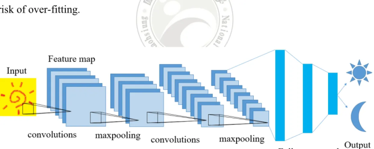
Like most deep learning methods, Convolutional neural network is designed to extract and analyze features; its general model example is shown as Figure 2.1. We can divide its structure into two parts. The first part extracts the features of data, whose structure consists of convolution layers and pooling layers. Usually, the input is represented as a matrix. The convolutional layers use filters to map the features of the input data onto a smaller matrix. Specifically, the filter will slide over the data. An area in the data is covered after each slide of the filter. If the data in this area is more similar to the features we need, the larger output will be generated.An example is shown in Figure 2.2. A convolutional layer can have multiple filters. More filters can increase the efficiency of identification, but require more computational cost and increase the risk of over-fitting.

(19)

10

Figure 2.2 An example of filter and feature extraction.

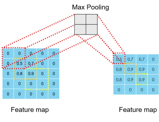
The main purpose of the pooling layer is to solve the problem of over-fitting caused by the convolutional layer. It also reduces the output size and helps to leave the required features. There are many ways to implement pooling, e.g., max pooling and mean pooling. Max pooling compares the pixels in the area, leaving the largest value, which can better preserve the texture features. An example is shown in Figure 2.3. Mean pooling replaces the pixels in the area with the regional mean to sustain the overall feature. Convolution layers and pooling layers will output multiple feature maps.

(20)

11

Figure 2.3 An example of max pooling.

The second part of CNN model is to analyze the features to answer the questions invoked by the user. The most adopted structure is to connect these feature maps to a multi-layered neuron called fully connected layer. After that, it will connect to the activation function to highlight the feature of the data which user needs through the conversion of the function. After these processes, the data become multiple values, and each value corresponds to a classification result. By comparing these values, it can be determined which class the data belongs to.

2.4 Related Work

In recent years, there have been many studies that analyze drug-related problems through machine learning algorithms. Jamal et al. [11] proposed a machine learning method to predict the adverse effects of drugs through the biological, chemical, and phenotypic properties of drugs provided by SIDER, DrugBank, and Pubchem [40] databases. Superior predictive outcomes were obtained in 22 neurologically relevant

(21)

12

symptoms (e.g., autonomic neuropathy, psychosis). This research demonstrated the association between the properties of drug and symptoms in different academic theory.

Burbidge et al. [3] used machine learning methods on drug design issues and used SVM to analyze quantitative structure-activity relationships (QSAR). SQAR is an idea that analyzes substances in pharmacy and chemistry, the relationship between structure of a molecule and activity or property of the substance. Duan et al. [6] proposed an ensemble method combining the likelihood ratio, BCPNN and Bayesian neural network.

There are also some studies based on deep learning. Unterthiner et al. [28] proposed a system called DeepTox that predicts the toxicity of drugs through inputting the chemical properties of the drug into a 5-layer deep neural network. Hughes et al. [10] studied the relationship between bonds in proteins and drug toxicity through deep convolutional neural networks. Wen et al. [31] proposed a method for predicting drug-target interaction (DTI). DTI helps to infer indications and adverse reactions during drug discovery. They screened the drugs first from the Drugbank database. Then use the documented construction model in the database. Their research helps to update the DTI list. Xu et al. [32] converted the structure of the drug to the SMILES form to predict the relationship of drug-induced liver injury (DILI). The study finally achieved 86.9% of accuracy. Park and Kellis [20] proposed to input DNA and RNA binding data into a deep learning network to calculate molecular affinity, which can be used to design drugs. Yao et al. [33] surveyed deep learning in Healthcare applications. The survey prompts some research directions and demonstrates the learning ability of convolutional neural networks.

(22)

13

Table 2.6 The state-of-the-art research

Model Target Dataset Method

PRR95 [22][25][35] Signal detection FAERS statistics ROR95 [22][25] Signal detection FAERS statistics MHRA [22] Signal detection FAERS statistics BCPNN [1][2][15] Signal detection FAERS statistics、

ML MGPS [25][34] Signal detection FAERS statistics、

ML Ensemble [6] Causal relationship OMOP statistics、 ML SMO [11] Causal relationship SIDER、 PubChem、 drugbank ML(SVM)

SVM-RBF [3] QSAR UCI Data

Repository ML(SVM) DeepTox [28] Toxicity

Prediction Tox21 DL

Hughes et al. [10] Toxicity

Prediction AMD DL

Wen et al. [31] update the DTI

list Drugbank DL DILI [32] Drug-induced liver injury prediction PaDEL DL

Park and Kellis [20] Drug discovery DeepBind DL(CNN)

In summary, we can find that previous work of using deep learning mostly analyzes the microscopic properties of drugs. There is no work to consider different levels in the Anatomical Therapeutic Chemical Classification System (ATC) [42] as shown in Table 2.7, which documents the classification of drugs under different perspectives. In the thesis we will explore the rich information provided by the drug's ATC code to predict specific adverse reactions.

(23)

14

Table 2.7. The meaning of ATC code

The first level A letter, representing the anatomical classification. The second level Two digits, representing the classification of therapeutics.

The third level A letter, representing the classification of pharmacological. The fourth level A letter, representing the classification of chemical.

(24)

15

Chapter 3 The Proposed Deep Learning ADR Prediction

Framework

In this chapter, we will describe the proposed deep learning-based framework for ADR prediction. Figure 3.1 depicts the framework structure. Each component is detailed in the following sections.

Figure 3.1 Proposed deep learning ADR detection framework

3.1 Preprocessing

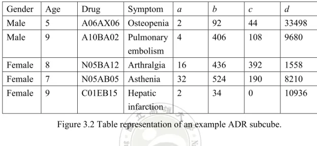
Rather than using the original FAERS data, we use the ADR contingency cubes built for our iADRs analysis system [17][18]. From the ADR cubes we chose the most

(25)

16

detailed subcube, composed of Age, Gender, Drug name, Symptom, and the four numerical values a, b, c, d, that record the values in the corresponding 2*2 contingency table for ADR detection. Note that Age is discretized into 10 levels and the drug is represented by ATC code. Figure 3.2 shows an example of this subcube represented in table format.

Gender Age Drug Symptom a b c d

Male 5 A06AX06 Osteopenia 2 92 44 33498

Male 9 A10BA02 Pulmonary embolism

4 406 108 9680

Female 8 N05BA12 Arthralgia 16 436 392 1558

Female 7 N05AB05 Asthenia 32 524 190 8210

Female 9 C01EB15 Hepatic infarction

2 34 0 10936

Figure 3.2 Table representation of an example ADR subcube.

Using this subcube as input data, the preprocessing module is to transfer it to a training set to build our deep learning network model. In the following subsections, we will explain the main procedures, including class labeling and disambiguation, class binarization, class imbalance handling, and the roles of MedDRA and SIDER in the preprocessing.

3.1.1 Class labeling

In Section 2.1 we mentioned that the casual relationship between drugs and adverse reactions in the FAERS reports has not been verified. This uncertainty hinders the construction of training set that requires correct class labels. To solve this problem, we utilize the well-known SIDER side effect resource (abbr. SIDER), which was proposed by Kuhn et al. in 2008 [13], containing side effects (adverse reactions)

(26)

17

information about marketed drugs. Its data is collected from FDA, national registries and charity organizations. It has recorded 1,430 drugs, 5,868 adverse reactions, and 139,756 drug-SE pairs. In the database, adverse reactions are represented by the PT layer and the LLT layer in MedDRA, and the drug name is available in versions encoded by the STITCH system [12] and in versions encoded by the ATC system. More specifically, we inspected all data in the ADR cubes and move all cases whose drug-ADR pair was found in SIDER to the data that will be processed to form the training set.

3.1.2 Class disambiguation

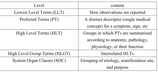
In the medical and healthcare community, professionals may use different words to record the observed symptoms. We need to standardize these words to ensure we can find all the cases about the specific symptom. As such, we used MedDRA database to solve this problem. MedDRA was developed by the International Council for Harmonisation of Technical Requirements for Pharmaceuticals for Human Use (ICH) and ICH partners, including WHO. It was designed to standardize the terminology required by regulators and industry, and is updated frequently to meet users’ requirement. MedDRA describes the symptom in five levels, as shown in Table 3.1.

(27)

18

Table 3.1Levels in MedDRA

Level content

Lowest Level Terms (LLT) How observations are reported Preferred Terms (PT) A distinct descriptor (single medical

concept) for a symptom, sign, etc High Level Terms (HLT) Groups in which PTs are summarized

according to anatomy, pathology, physiology, or their function High Level Group Terms (HLGT) Interrelated HLTs

System Organ Classes (SOC) Grouping of etiology, manifestation site, and purpose

LLTs contain many synonyms. So we describe the symptoms with PTs at first. However, when we target a specific symptom, only a few cases were found to meet our needs. This will have a negative impact on the learning of the model. So, we try to describe the symptoms using a higher level. In order to keep the groups of symptoms close to meaningful synonyms, we chose the upper layer of PT, i.e. HLT.

3.1.3 Class binarization

In nature, the problem of ADR prediction is a multi-class classification task since a drug may cause many different adverse reactions, but for the following reason we transfer it into a binary class problem. Recall that the adverse reactions recorded in the SRS system are uncertain, which makes it more difficult to determine the right combination of adverse reactions when constructing the training dataset. We thus adopted the one-to-the-others strategy. That is, for each specific adverse reaction, we will build a binary classification model to predict that when a patient takes a particular drug, he will suffer the specific adverse reaction or not. For example, if we want to predict whether myocardial infarction will occur after a patient takes a specific drug,

(28)

19

we will use all cube instances that record myocardial infarction as positive cases, while all cube instances that record of other PTs as negative cases, as illustrated in Figure 3.3. However, this will make the set of negative cases much larger than that of the positive cases, because there may be many kinds of adverse reactions after taking a drug, and the specific case we focus on is only one of them. This problem will be handled in the next subsection. There is another phenomenon needs special attention. Since a drug may cause more than one adverse reaction, it is very likely that after class binarization, the drug will belong to both positive and negative classes. Since our focus is on the positive case, identifying the drug causing the adverse reaction of concern, the existence of the drug in the negative class will perplex the binary model to conclude the positive decision. We name such kind of negative cases as perplexing negatives. A simple solution is eliminating the perplexing negatives from the training set. For example, in Figure 3.3, instances 2 to 5 will be eliminated. The effect of pruning perplexing negatives will be shown later in Section 4.2.

(29)

20

3.1.4 Class imbalance handling

After the class binariztion, all instances in the ADR cube are divided into two categories: those that produce the specific adverse reaction and those that do not produce the specific adverse reaction. Note that the size of the second category is significantly larger than that of the first one. For example, in the data of 2004-2006, there are only 3,521 cube instances that record myocardial infarction, but there are 672,297 instances that record other adverse reactions. This is the well-known class imbalance problem which will cause the learned model exhibit very low accuracy for the rare class.

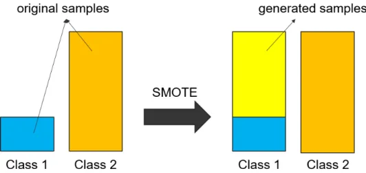
To solve this problem, we used the SMOTE [5] approach to oversample the rare category that corresponds to the specific adverse reaction of concern. The SMOTE approach generates samples of rare class to balance the sample, as shown in Figure 3.4. More specifically, SMOTE randomly selects a sample of rare class S1, finds the K-nearest samples of S1 of the same class, randomly selects one sample S2 from the K-nearest samples of S1, and generates a sample S3 which is between S1 and S2. An example is given in Figure 3.5. SMOTE will repeat this process until the classes are balance.

(30)

21

Figure 3.5 A depiction of the SMOTE approach.

In the SMOTE approach, we need to calculate the similarity between any two cube instances. We use different calculation methods for different types of attributes. For binary attribute like Gender, if the values of the two instances are the same, we set the similarity to 1, otherwise, set to 0. Because Age is an ordinal attribute with 10 levels, we normalize the similarity between the two instances by dividing the value by 10. Special attention should be made for Drug, because Drug is represented by ATC code, which itself contains five different components. We thus divide it to five components, and calculate the similarity by counting the individual similarity of each component. An example is shown in Figure 3.6.

(31)

22

3.2 Model Building

In this section, we show the structure of the deep learning model and how we convert the data into the input of the model. Note that the input data are from the ADR cube in which each instance corresponds to a specific group of patients that take a specific drug along with the statistics in the contingency table. We want to preserve the statistical properties of the data and to analyze it along with the patient's attributes.

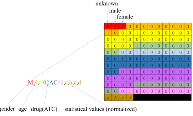
3.2.1 Data transformation

In order to make the data available as an input to the convolutional neural network, we need to convert the data into a matrix. The Age, Gender, Drug (ATC code), Adverse Reaction, and statistics in the contingency table are recorded in our data. For categorical attributes such as Age, Gender, and Drug, we convert them to the input matrix in one-hot encoding. That is, the content of each variable is converted into a binary vector whose length equals to the cardinality of the variable domain, with each position denoting the presence of the corresponding value. For example, the domain of Gender variable is {unknown, male, female}. So it is transferred to a binary vector of length 3, the first position corresponding to value “unknown”, the second to value “male”, and third to “female”. The statistical values a, b, c, d in the contingency table are normalized to [0, 1] and input directly into the input matrix. An example is shown in Figure 3.7, where attribute Age is converted to a vector of length 10 because there are 10 levels, and so are the other attributes. As for the output class, i.e., Adverse Reaction, we convert it into a 1*2 matrix. If it is the specific adverse reaction we focus on, we set the first item to 1 and the second item to 0. Otherwise, the first item is set to 0 and the second item is set to 1.

(32)

23

Figure 3.7 An example transformation of input string to matrix. The input value is transferred to the vector with the same color in the matrix.

3.2.2 Model structure

Figure 3.8 shows our model structure, which is composed of two main subnetworks: convolutional network and fully connected network. The matrix we mentioned in subsection 3.2.1 is the input of the model. Features of the input matrix are extracted through the first part that contains several convolutional layers and a pooling layer. Size and number of the convolutional layers and the presence or absence of the pooling layer will affect the extraction of features and the predicted results. Therefore, we conducted experiments to determine the best structure, which will be described in Section 4.3. Next, the features are passed to the fully connected layer and become several values which decide the input would cause ADR or not. Finally, we added a softmax function to make the answer of the model clearer. The answer is also used to calculate the loss function. The loss function we use is binary cross entropy,which is shown in equation (3.1), because our model is used to answer the binary classification.

(33)

24

Figure 3.8 The proposed CNN-based model structure

Loss = − _{𝑁𝑁 �[𝑦𝑦}1 𝑖𝑖log(𝑦𝑦�) + (1 − 𝑦𝑦𝚤𝚤 𝑖𝑖)log (1 − 𝑦𝑦�)]𝚤𝚤 𝑁𝑁

𝑖𝑖=1

(3.1)

where Loss represents the value that used to modify the model, N represents the number of instances in a batch, 𝑦𝑦𝑖𝑖 represents the probability of true label which is ground truth, and 𝑦𝑦� represents the probability of label that the model predicted. 𝚤𝚤

(34)

25

Chapter 4 Experimental Results

In this chapter, we will describe our experiments. First, we describe the experimental design, including the data set, the choice of symptoms and drugs, and the computing environment. Second, we conduct an experiment to see the effect of pruning perplexing negatives cases. Third, we present an experiment on the choice of parameters and model structure for our proposed CNN-based model, followed by the experiment to inspect how the constructed training set affects the performance of the learned CNN-based model. Finally, we conducted a series of experiments to examine the performance of the learned CNN-model on ADR detection.

4.1 Experimental Design

We chose the ADR cubes from our iADRs system that ranges from 2004 to 2016, using the subcubes between 2004 and 2006 as training set and the others as testing set. The timing granularity is quarter, following that used by FAERS. In total, there are 675,818 cube instances.

All experiments were conducted on a PC workstation, equipped with 16GB main memory, 1TB hard disk, Intel core i7-8700 CPU, NVIDIA GeForce RTX 2060 6GB GPU, and running Windows 10 operating system. All programs were coded in python, using tensorflow, keras and numpy package. Our proposed method requires a specific adverse reaction. We chose myocardial infarction because it is dangerous and fatal. To evaluate the performance of our model in ADR detection, we selected from MedWatch 7 drugs that were not listed in SIDER but did cause myocardial infarction. Table 4.1 shows the details of these 7 drugs.

(35)

26

Table 4.1 Summary of the chosen drugs for ADR detection.

Drug Name Warning Date Marketing Date

tegaserod Quarter 4, 2007 Quarter 1, 2004

olmesartan Quarter 2, 2010 Quarter 1, 2004

leuprorelin Quarter 2, 2010 Quarter 1, 2004 rosiglitazone Quarter 4, 2010 Quarter 1, 2004

abacavir Quarter 1, 2011 Quarter 1, 2004

testosterone Quarter 1, 2014 Quarter 1, 2004

omalizumab Quarter 3, 2014 Quarter 1, 2004

* If the drug was marketed before FAERS was established, we set the Marketing Date as Quarter 1 of 2004, the date FAERS established.

4.2 Effect of Perplexing Negatives

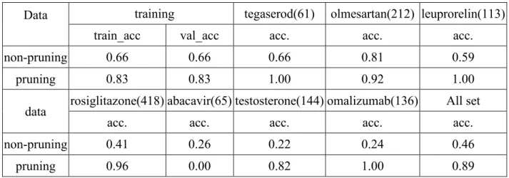
In this section, we present the experiment we conducted to examine the effect of perplexing negatives. To this end, two models were trained; one of them was trained without pruning the perplexing negative cases, and another one was trained by pruning the perplexing negatives. We considered the seven drugs listed in Table 4.1 to evaluate the performance of these two models. Table 4.2 shows the results where the training, validation and testing accuracies of two models are recorded. As the results demonstrate, only 0.66 of accuracy was obtained for the model without pruning the perplexing negatives, for training and validation, while the accuracy can reach 0.83 for the model with pruning. Similar results were observed for the testing accuracies. On average, the testing accuracy only reaches 0.46 without pruning while it reaches 0.89 with pruning.

(36)

27

Table 4.2 The performance of model trained by pruning/non-pruning perplexing negatives cases.

Data training tegaserod(61) olmesartan(212) leuprorelin(113)

train_acc val_acc acc. acc. acc.

non-pruning 0.66 0.66 0.66 0.81 0.59

pruning 0.83 0.83 1.00 0.92 1.00

data rosiglitazone(418) abacavir(65) testosterone(144) omalizumab(136) All set

acc. acc. acc. acc. acc.

non-pruning 0.41 0.26 0.22 0.24 0.46

pruning 0.96 0.00 0.82 1.00 0.89

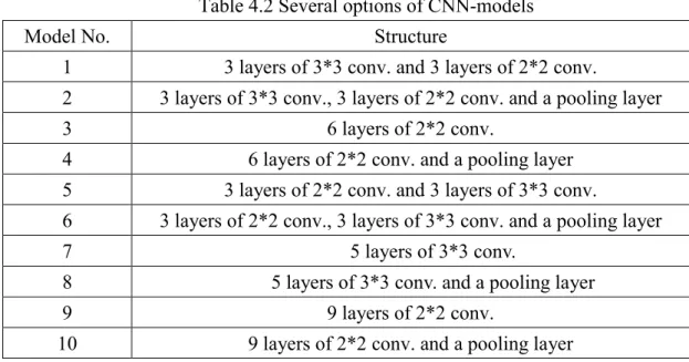
4.3 Model Selection

In this section, we describe the experiments to determine the structure and parameters of our proposal CNN-based model. To this end, we considered several options as shown in Table 4.2. Totally, there are 10 options. We considered the drugs listed in Table 4.1 to evaluate the performance of these 10 model options on predicting the ADR myocardial infarction. Two different levels of symptoms were inspected in our experiments; they are PT level and HLT level in MedDRA. Table 4.3 shows the results, where the training, validation and testing accuracies of the ten models are recorded. Among them, model 2 exhibits the best testing performance for both levels of symptoms, followed by models 3 and 7.

(37)

28

Table 4.2 Several options of CNN-models

Model No. Structure

1 3 layers of 3*3 conv. and 3 layers of 2*2 conv.

2 3 layers of 3*3 conv., 3 layers of 2*2 conv. and a pooling layer

3 6 layers of 2*2 conv.

4 6 layers of 2*2 conv. and a pooling layer 5 3 layers of 2*2 conv. and 3 layers of 3*3 conv.

6 3 layers of 2*2 conv., 3 layers of 3*3 conv. and a pooling layer

8 5 layers of 3*3 conv. and a pooling layer

10 9 layers of 2*2 conv. and a pooling layer

Table4.3 The performance of different CNN-models.

Model No. training tegaserod(61) olmesartan(212) leuprorelin(113)

train_acc val_acc acc. acc. acc.

PT Model1 0.86 0.86 1.00 0.91 1.00 Model2 0.87 0.87 1.00 1.00 1.00 Model3 0.86 0.86 1.00 0.78 1.00 Model4 0.86 0.86 1.00 1.00 1.00 Model5 0.85 0.85 1.00 0.93 1.00 Model6 0.86 0.85 1.00 1.00 1.00 Model7 0.86 0.86 1.00 1.00 0.99 Model8 0.91 0.91 0.48 1.00 1.00 Model9 0.84 0.84 1.00 0.78 1.00 Model10 0.85 0.86 0.11 1.00 0.99 HLT Model1 0.80 0.80 1.00 0.97 0.99 Model2 0.83 0.83 1.00 0.92 1.00 Model3 0.81 0.81 1.00 1.00 1.00 Model4 0.82 0.82 0.49 0.01 0.44 Model5 0.80 0.80 1.00 0.97 0.99 Model6 0.83 0.83 0.57 0.00 0.27 Model7 0.81 0.80 1.00 1.00 1.00 Model8 0.86 0.87 0.97 0.51 0.27 Model9 0.80 0.80 1.00 1.00 1.00 Model10 0.82 0.82 0.00 1.00 1.00

(38)

29

Table 4.3 (continues) Model

No.

rosiglitazone(418) abacavir(65) testosterone(144) omalizumab(136) All set

acc. acc. acc. acc. acc.

PT Model1 0.97 0.31 0.03 0.01 0.69 Model2 0.97 0.00 0.00 1.00 0.81 Model3 0.89 0.11 0.02 0.01 0.63 Model4 0.89 0.23 0.03 0.01 0.68 Model5 0.89 0.26 0.04 0.01 0.67 Model6 0.00 0.00 0.00 0.00 0.34 Model7 0.86 0.06 0.02 0.01 0.65 Model8 0.00 0.02 0.05 0.04 0.32 Model9 0.89 0.11 0.02 0.01 0.63 Model10 0.99 0.00 0.00 0.00 0.65 HLT Model1 0.69 0.45 0.76 0.09 0.71 Model2 0.96 0.00 0.82 1.00 0.89 Model3 0.77 0.88 0.93 0.53 0.85 Model4 0.74 0.58 0.28 0.01 0.41 Model5 0.74 0.78 0.74 0.32 0.78 Model6 0.00 0.00 0.00 0.00 0.06 Model7 0.84 0.85 0.93 0.37 0.85 Model8 0.00 0.02 0.00 0.00 0.17 Model9 0.83 0.69 0.92 0.13 0.81 Model10 0.94 0.02 0.44 0.99 0.80

4.4 Models Trained by SIDER Alone

Our approach constructed the CNN-model using FAERS data and SIDER as the background knowledge of drugs and adverse reactions. An interesting question is the role of SIDER. Can we use it as the training set to learn a model and how well it perform? For this purpose, we use SIDER to build the model directly. Specifically, we still use the proposed model. Since there is no Gender, Age and statistical values recorded in SIDER, we entered 0 as unknown value. We divided the SIDER into 9:1. Then use the larger part as the training set, of which 70% was used for training and 30% was used

(39)

30

for validation. The small part was used as a test set. The results of the experiment are shown in Table 4.4. Clearly, the results are inferior to the results obtained by our approach.

Table 4.4 Model accuracy by using SIDER alone as training set Model

No.

Training Test-set

train_acc val_acc SIDER-Myocardial infarction PT 2 0.76 0.73 0.58 3 0.75 0.69 0.55 7 0.74 0.68 0.56 HLT 2 0.84 0.83 0.68 3 0.75 0.75 0.57 7 0.75 0.76 0.55

Another interesting question is: How will the performance become if we used an older version of SIDER, e.g., SIDER 2.0, as the training set to learn a model to test the new rules listed in a newer version of SIDER, i.e., SIDER 4.0. As the results shown in Table 4.5, a very bad performance, around 44% of accuracy, was observed in the testing set.

Table 4.5 Model accuracy by using older version of SIDER to predict new rules in the current version

Model No.

Training Test-set

train_acc val_acc SIDER-Myocardial infarction PT 2 0.80 0.79 0.46 3 0.73 0.72 0.55 7 0.72 0.77 0.41 HLT 2 0.88 0.86 0.44 3 0.73 0.73 0.42 7 0.73 0.73 0.38

(40)

31

Both experiments show that it is not appropriate to use SIDER alone to train a deep learning model. The main reason may be due to its restricted size.

4.5 Model Evaluation

To evaluate the performance of our proposed model on ADR detection, we considered the seven drugs in Table 4.1. We used the ADR cube ranging from 2007 to 2016 as the testing set. Based on the results in Section 4.3, we chose models 2, 3 and 7. Our purpose in this experiment is to evaluate:

(1) Whether our models can detect the known 7 ADR signals, and

(2) How early our models can detect the signals, compared with statistics-based approaches and the FDA warning time.

For this purpose, we computed and recorded for all signals the accuracy (the percentage that our models answer yes) that our models can generate in each quarter. For example, consider Table 4.6, the results of model 2 in the PT level. The value in each cell of the table represents how many percentage of the records in the corresponding quarter that our model can generate the corresponding signal. For convenience, we highlight the time stamp with yellow that FDA released the warning of that ADR and with orange the earliest time that our model generated the signal. N represents there was no report observing myocardial infarction after taking the drug in that quarter.

To observe whether a signal can be generated by our model, we need to determine a threshold for the accuracy. That is, to what extent of the accuracy that the ADR signal can be considered as valid. Rather than leaving the threshold to the user, we specify the value based on the statistical concept of confidence interval. According to the

(41)

32

commonly used 95% of confidence, we can derive the threshold that is significantly far beyond the average accuracy, as follows:

θ = μ �1 + 𝜎𝜎

√𝑛𝑛� + 1.96 ∗ 𝜎𝜎2

√𝑛𝑛 (4.1)

where μ is the average accuracy and σ is the sample deviation.

As the results shown in Tables 4.6 to 4.11, in most cases, our models can detect ADR signal before FDA release warnings. Furthermore, HLT-Model 3 and HLT-Model 7 successfully detect all the 7 signals before FDA released the alerts. On average, both HLT-Model 3 and HLT-Model 7 detect the signals 16 quarters earlier than FDA released the alerts.

Table 4.6 Timeline ADR detection results of PT-Model 2 PT-Model 2, μ=0.71 , θ= 0.76

Year Quarter tegaserod olmesartan leuprorelin rosiglitazone abacavir testosterone omalizumab

2007 Q1 1 1 1 1 N 0 1 Q2 1 1 1 0.9 N 0 1 Q3 1 1 1 1 N 0 1 Q4 1 1 1 1 N N 1 2008 Q1 1 1 1 1 N 0 N Q2 1 1 1 1 0 0 N Q3 N 1 1 1 0 0 1 Q4 1 1 1 1 0 0 1 2009 Q1 1 1 1 1 0 0 N Q2 1 1 1 1 0 0 1 Q3 1 1 1 1 0 0 1 Q4 1 1 1 0.92 0 0 1 2010 Q1 1 1 1 1 0 0 1 Q2 1 1 1 0.93 0 0 1 Q3 N 1 1 1 0 0 1 Q4 1 1 1 1 0 0 1 2011 Q1 N 1 1 0.92 0 0 1 Q2 1 1 1 1 0 0 1 Q3 1 1 1 1 0 0 1

(42)

33

Table 4.6 (continues)

PT-Model 2, μ=0.71 , θ= 0.76

2012 Q1 N 1 1 0.93 N 0 1 Q2 1 1 1 0.86 0 0 1 Q3 N 1 1 1 0 0 1 Q4 N 1 1 0.92 0 0 1 2013 Q1 N 1 1 0.92 N 0 1 Q2 N 1 1 1 N 0 1 Q3 N 1 1 1 0 0 1 Q4 N 1 1 1 0 0 1 2014 Q1 N 1 1 0.93 0 0 1 Q2 N 1 1 1 0 0 1 Q3 1 1 1 1 0 0 1 Q4 N 1 1 0.94 0 0 1 2015 Q1 N 1 1 0.94 0 0 1 Q2 N 1 1 1 0 0 1 Q3 N 1 1 1 N 0 1 Q4 N 1 1 1 0 0 1 2016 Q1 N 1 1 1 0 0 1 Q2 N 1 1 1 0 0 1 Q3 N 1 1 1 N 0 1 Q4 N 1 1 1 0 0 1

(43)

34

2007 Q1 1 0.75 1 1 N 0 0 Q2 1 0 1 0.9 N 0 0 Q3 1 1 1 1 N 0 0 Q4 1 1 1 0.92 N N 0 2008 Q1 1 1 1 1 N 0 N Q2 1 0.67 1 1 0 0 N Q3 N 1 1 1 0 0 0 Q4 1 1 1 0.9 0 0 0 2009 Q1 1 1 1 1 0 0 N Q2 1 0.75 1 1 0.5 0 0 Q3 1 1 1 0.92 0 0 0 Q4 1 0.875 1 0.92 0 0 0 2010 Q1 1 0.8 1 1 0 0 0 Q2 1 0.8 1 0.73 0 0 0 Q3 N 0.8 1 0.92 1 0 0 Q4 1 0.8 1 0.92 0 0 0 2011 Q1 N 0.67 1 0.92 0 0 0 Q2 1 1 1 0.92 0.5 0 0 Q3 1 0.57 1 1 0 0 0 Q4 1 0.83 1 0.92 0 0 0

(44)

35

PT-Model 3, μ=0.54 , θ= 0.58

2012 Q1 N 0.57 1 0.8 N 0 0 Q2 1 0.86 1 0.79 0 0 0 Q3 N 0.71 1 0.91 0 0 0 Q4 N 0.67 1 0.92 0 0 0 2013 Q1 N 0.71 1 0.83 N 0 0 Q2 N 0.57 1 1 N 0 0 Q3 N 0.86 1 1 0 0 0 Q4 N 0.5 1 0.9 0 0 0 2014 Q1 N 0.8 1 0.71 0 0 0 Q2 N 0.5 1 0.71 0 0.14 0 Q3 1 0.71 1 0.8 1 0 0 Q4 N 0.8 1 0.75 0.5 0 0 2015 Q1 N 0.7 1 0.69 1 0.25 0.2 Q2 N 0.86 1 0.91 0 0 0 Q3 N 0.8 1 0.86 N 0 0 Q4 N 0.86 1 1 0 0 0 2016 Q1 N 0.75 1 1 0 0 0 Q2 N 0.88 1 1 0 0 0 Q3 N 0.83 1 1 N 0 0 Q4 N 0.8 1 1 0 0 0

(45)

36

2007 Q1 1 1 1 1 N 0 0 Q2 1 1 1 0.9 N 0 0 Q3 1 1 1 1 N 0 0 Q4 1 1 1 0.92 N N 0 2008 Q1 1 1 1 1 N 0 N Q2 1 1 1 1 0 0 N Q3 N 1 1 1 0 0 0 Q4 1 1 1 0.9 0 0 0 2009 Q1 1 1 1 1 0 0 N Q2 1 1 1 0.91 0 0 0 Q3 1 1 1 0.83 0 0 0 Q4 1 1 1 0.83 0 0 0 2010 Q1 1 1 1 0.91 0 0 0 Q2 1 1 1 0.73 0 0 0 Q3 N 1 1 0.92 1 0 0 Q4 1 1 1 0.92 0 0 0 2011 Q1 N 1 1 0.92 0 0 0 Q2 1 1 1 0.92 0 0 0 Q3 1 1 0.75 0.91 0 0 0 Q4 1 1 1 0.92 0 0 0

(46)

37

PT-Model 7, μ=0.56 , θ= 0.61

2012 Q1 N 1 1 0.73 N 0 0 Q2 1 1 1 0.79 0 0 0 Q3 N 1 1 0.91 0 0 0 Q4 N 1 1 0.92 0 0 0 2013 Q1 N 1 1 0.83 N 0 0 Q2 N 1 1 0.91 N 0 0 Q3 N 1 1 0.91 0 0 0 Q4 N 1 1 0.9 0 0 0 2014 Q1 N 1 1 0.71 0 0 0 Q2 N 1 1 0.64 0 0.14 0 Q3 1 1 1 0.73 1 0 0 Q4 N 1 1 0.63 0 0 0 2015 Q1 N 1 1 0.63 1 0.25 0.2 Q2 N 1 1 0.91 0 0 0 Q3 N 1 1 0.86 N 0 0 Q4 N 1 1 1 0 0 0 2016 Q1 N 1 1 1 0 0 0 Q2 N 1 1 1 0 0 0 Q3 N 1 1 1 N 0 0 Q4 N 1 1 1 0 0 0

(47)

38

Table 4.9 Timeline ADR detection results of HLT-Model 2 HLT-Model 2, μ=0.84 , θ= 0.87

2007 Q1 1 1 1 1 N 1 1 Q2 1 1 1 0.9 N 1 1 Q3 1 1 1 1 N 1 1 Q4 1 1 1 1 N N 1 2008 Q1 1 1 1 1 N 1 N Q2 1 1 1 1 0 1 N Q3 N 1 1 1 0 1 1 Q4 1 1 1 1 0 1 1 2009 Q1 1 1 1 1 0 1 N Q2 1 1 1 1 0 1 1 Q3 1 1 1 1 0 1 1 Q4 1 0.88 1 0.92 0 1 1 2010 Q1 1 1 1 1 0 1 1 Q2 1 1 1 0.87 0 1 1 Q3 N 1 1 1 0 0.5 1 Q4 1 1 1 1 0 0.67 1 2011 Q1 N 0.67 1 0.92 0 0.8 1 Q2 1 1 1 1 0 1 1 Q3 1 0.71 1 1 0 1 1 Q4 1 1 1 0.92 0 1 1

(48)

39

HLT-Model 2, μ=0.84 , θ= 0.87

2012 Q1 N 0.71 1 0.93 N 1 1 Q2 1 0.86 1 0.86 0 0.75 1 Q3 N 0.86 1 1 0 1 1 Q4 N 1 1 0.92 0 1 1 2013 Q1 N 1 1 0.92 N 1 1 Q2 N 0.86 1 1 N 1 1 Q3 N 0.86 1 1 0 1 1 Q4 N 0.83 1 1 0 0.75 1 2014 Q1 N 1 1 0.93 0 0.71 1 Q2 N 1 1 0.93 0 0.71 1 Q3 1 0.86 1 0.93 0 0.57 1 Q4 N 1 1 0.88 0 0.71 1 2015 Q1 N 0.9 1 0.88 0 0.62 1 Q2 N 1 1 1 0 0.86 1 Q3 N 1 1 1 N 0.83 1 Q4 N 1 1 1 0 0.71 1 2016 Q1 N 1 1 1 0 0.75 1 Q2 N 0.88 1 1 0 0.83 1 Q3 N 1 1 1 N 0.75 1 Q4 N 0.8 1 1 0 0.8 1

(49)

40

2007 Q1 1 1 1 1 N 1 0 Q2 1 1 1 0.7 N 1 0 Q3 1 1 1 0.9 N 1 1 Q4 1 1 1 0.75 N N 0.5 2008 Q1 1 1 1 1 N 1 N Q2 1 1 1 0.75 1 1 N Q3 N 1 1 0.73 0.5 1 0 Q4 1 1 1 0.7 0.8 1 1 2009 Q1 1 1 1 0.73 0.8 1 N Q2 1 1 1 0.73 1 1 1 Q3 1 1 1 0.67 1 1 0.29 Q4 1 1 1 0.67 0.5 1 0.67 2010 Q1 1 1 1 0.73 0.67 1 1 Q2 1 1 1 0.6 1 1 0.5 Q3 N 1 1 0.83 1 1 0.5 Q4 1 1 1 0.83 1 1 0.25 2011 Q1 N 1 1 0.83 1 1 0.25 Q2 1 1 1 0.83 1 1 0.5 Q3 1 1 1 0.82 1 1 0 Q4 1 1 1 0.83 1 1 0.75

(50)

41

HLT-Model 3, μ=0.88 , θ= 0.90

2012 Q1 N 1 1 0.73 N 1 0.67 Q2 1 1 1 0.79 1 1 0.67 Q3 N 1 1 0.82 1 1 0.25 Q4 N 1 1 0.83 1 1 0.5 2013 Q1 N 1 1 0.83 N 1 0.6 Q2 N 1 1 0.82 N 1 0.5 Q3 N 1 1 0.91 1 1 0.4 Q4 N 1 1 0.9 1 1 0.8 2014 Q1 N 1 1 0.71 1 0.86 1 Q2 N 1 1 0.71 1 0.86 0.75 Q3 1 1 1 0.67 1 0.71 0.6 Q4 N 1 1 0.62 1 0.86 1 2015 Q1 N 1 1 0.69 1 0.75 0.8 Q2 N 1 1 0.91 1 1 1 Q3 N 1 1 0.86 N 1 0.71 Q4 N 1 1 1 0.67 0.86 0.14 2016 Q1 N 1 1 0.83 1 0.75 0.29 Q2 N 1 1 1 1 1 0.4 Q3 N 1 1 0.5 N 1 0.5 Q4 N 1 1 1 1 1 0.67

(51)

42

2007 Q1 1 1 1 1 N 1 0 Q2 1 1 1 0.8 N 1 0 Q3 1 1 1 1 N 1 1 Q4 1 1 1 0.75 N N 0 2008 Q1 1 1 1 1 N 1 N Q2 1 1 1 1 1 1 N Q3 N 1 1 0.82 0.5 1 0 Q4 1 1 1 0.8 0.8 1 0 2009 Q1 1 1 1 0.82 0.8 1 N Q2 1 1 1 0.82 1 1 1 Q3 1 1 1 0.75 1 1 0.29 Q4 1 1 1 0.75 0.5 1 0.67 2010 Q1 1 1 1 0.82 0.67 1 1 Q2 1 1 1 0.67 0.33 1 0 Q3 N 1 1 0.92 1 1 0.5 Q4 1 1 1 0.92 0.5 1 0.25 2011 Q1 N 1 1 0.83 1 1 0 Q2 1 1 1 0.83 1 1 0.5 Q3 1 1 1 0.91 1 1 0 Q4 1 1 1 0.83 1 1 0.5

(52)

43

HLT-Model 7, μ=0.86 , θ= 0.89

2012 Q1 N 1 1 0.73 N 1 0 Q2 1 1 1 0.79 1 1 0.33 Q3 N 1 1 0.91 1 1 0.25 Q4 N 1 1 0.92 1 1 0 2013 Q1 N 1 1 0.92 N 1 0.4 Q2 N 1 1 1 N 1 0.5 Q3 N 1 1 1 1 1 0.2 Q4 N 1 1 1 1 1 0.4 2014 Q1 N 1 1 0.79 1 0.86 0.5 Q2 N 1 1 0.79 1 0.86 0.5 Q3 1 1 1 0.73 1 0.71 0.6 Q4 N 1 1 0.69 1 0.86 1 2015 Q1 N 1 1 0.69 1 0.75 0.8 Q2 N 1 1 1 1 1 1 Q3 N 1 1 0.86 N 1 0.71 Q4 N 1 1 1 0.67 0.86 0 2016 Q1 N 1 1 1 1 0.75 0.29 Q2 N 1 1 1 1 1 0 Q3 N 1 1 0.5 N 1 0.33 Q4 N 1 1 1 1 1 0.67

According to these results, HLT-Model 3 exhibits the overall best performance. We further depict the results as line charts in Figure 4.1 to Figure 4.7.

(53)

44

Figure 4.1 Line chart of HLT-Model 3 on detecting tegaserod ADR signal.

Figure 4.2 Line chart of HLT-Model 3 on detecting olmesartan ADR signal.

0

0.5

1

1.5

07Q 1 07Q 4 08Q 3 09Q 2 10Q 1 10Q 4 11Q 3 12Q 2 13Q 1 13Q 4 14Q 3 15Q 2 16Q 1 16Q 4

HLT-Model3 tegaserod

Acc.

θ

0.8

0.9

1

1.1

07Q 1 07Q 4 08Q 3 09Q 2 10Q 1 10Q 4 11Q 3 12Q 2 13Q 1 13Q 4 14Q 3 15Q 2 16Q 1 16Q 4

HLT-Model3 olmesartan

Acc.

θ

(54)

45

Figure 4.3 Line chart of HLT-Model 3 on detecting leuprorelin ADR signal.

Figure 4.4 Line chart of HLT-Model 3 on detecting rosiglitazone ADR signal.

0.8

0.9

1

1.1

07Q 1 07Q 4 08Q 3 09Q 2 10Q 1 10Q 4 11Q 3 12Q 2 13Q 1 13Q 4 14Q 3 15Q 2 16Q 1 16Q 4

HLT-Model3 leuprorelin

Acc.

θ

0

0.5

1

1.5

07Q 1 07Q 4 08Q 3 09Q 2 10Q 1 10Q 4 11Q 3 12Q 2 13Q 1 13Q 4 14Q 3 15Q 2 16Q 1 16Q 4

HLT-Model3 rosiglitazone

Acc.

θ

(55)

46

Figure 4.5 Line chart of HLT-Model 3 on detecting abacavir ADR signal.

Figure 4.6 Line chart of HLT-Model 3 detecting testosterone ADR signal.

0

0.5

1

1.5

07Q 1 07Q 4 08Q 3 09Q 2 10Q 1 10Q 4 11Q 3 12Q 2 13Q 1 13Q 4 14Q 3 15Q 2 16Q 1 16Q 4

HLT-Model3 abacavir

Acc.

θ

0

0.5

1

1.5

07Q 1 07Q 4 08Q 3 09Q 2 10Q 1 10Q 4 11Q 3 12Q 2 13Q 1 13Q 4 14Q 3 15Q 2 16Q 1 16Q 4

HLT-Model3 testosterone

Acc.

θ

(56)

47

Figure 4.7 Line chart of HLT-Model 3 detecting omalizumab ADR signal.

Finally, we compare the results of HLT-Model3, with the classical signal detection methods such as PRR95, ROR95, IC, MHRA, SPRT [28], and Yule's Q [7]. To emulate the situation that all seven considered drugs are newly marketed and see how statistics-based approaches will perform, we only use FAERS data after 2007Q1 for measuring statistics-based approaches. The results are shown in Table 4.12 to Table 4.18, where number “1” represents that ADR signal is generated, number “0” represents the ADR signal is not generated, “N” represents there is no case that taking the specific drug and occurring myocardial infarction in that quarter. We highlight the timestamp with yellow that FDA released the warning of that ADR, with orange the earliest time that our model generated the signal and with green the earliest time that classical methods generated the signal. The results show that nearly all statistics-based methods generate signals before FDA’s warnings, except MHRA and SPRT, which fails to generate signals for drug “Leuprorelin”. Our method outperforms all statistics-based methods. IC exhibits the best performance, but two quarters behind our method on average.

0

0.5

1

1.5

07Q 1 07Q 4 08Q 3 09Q 2 10Q 1 10Q 4 11Q 3 12Q 2 13Q 1 13Q 4 14Q 3 15Q 2 16Q 1 16Q 4

HLT-Model3 omalizumab

Acc.

θ

(57)

48

Table 4.12 Timeline ADR detection results of classical methods for detecting tegaserod

Date PRR95 ROR95 IC MHRA SPRT Yule’s Q

07Q1 0 0 0 0 0 0 07Q2 1 1 1 1 1 1 07Q3 1 1 1 1 1 1 07Q4 1 1 1 1 1 1 08Q1 0 0 1 0 0 0 08Q2 1 1 1 1 0 1 08Q3 N N N N N N 08Q4 1 1 1 1 0 1 09Q1 1 1 1 1 1 1 09Q2 1 1 1 1 1 1 09Q3 0 0 1 0 0 0 09Q4 1 1 1 1 1 1 10Q1 1 1 1 1 1 1 10Q2 1 1 1 1 1 1 10Q3 N N N N N N 10Q4 1 1 1 1 1 1 11Q1 N N N N N N 11Q2 1 1 1 1 1 1 11Q3 1 1 1 1 1 1 11Q4 1 1 1 1 0 1 12Q1 N N N N N N

(58)

49

12Q2 1 1 1 1 1 1 12Q3 N N N N N N 12Q4 N N N N N N 13Q1 N N N N N N 13Q2 N N N N N N 13Q3 N N N N N N 13Q4 N N N N N N 14Q1 N N N N N N 14Q2 N N N N N N 14Q3 1 1 1 0 0 1 14Q4 N N N N N N 15Q1 N N N N N N 15Q2 N N N N N N 15Q3 N N N N N N 15Q4 N N N N N N 16Q1 N N N N N N 16Q2 N N N N N N 16Q3 N N N N N N 16Q4 N N N N N N

(59)

50

Table 4.13 Timeline ADR detection results of classical methods for detecting olmesartan

07Q1 0 0 1 0 0 0 07Q2 0 0 0 0 0 0 07Q3 0 0 0 0 0 0 07Q4 0 0 1 0 0 0 08Q1 0 0 1 0 0 0 08Q2 0 0 0 0 0 0 08Q3 0 0 1 0 0 0 08Q4 0 0 0 0 0 0 09Q1 0 0 1 0 0 0 09Q2 0 0 0 0 0 0 09Q3 0 0 1 0 0 0 09Q4 1 1 1 0 1 1 10Q1 0 0 1 0 0 0 10Q2 0 0 1 0 0 0 10Q3 0 0 0 0 0 0 10Q4 0 0 0 0 0 0 11Q1 0 0 1 0 0 0 11Q2 0 0 0 0 0 0 11Q3 0 0 1 0 0 0 11Q4 0 0 0 0 0 0 12Q1 0 0 0 0 0 0

(60)

51

12Q2 0 0 1 0 0 0 12Q3 0 0 0 0 0 0 12Q4 0 0 0 0 0 0 13Q1 0 0 1 0 0 0 13Q2 1 1 1 0 0 1 13Q3 0 0 0 0 0 0 13Q4 0 0 1 0 0 0 14Q1 0 0 1 0 0 0 14Q2 0 0 0 0 0 0 14Q3 0 0 0 0 0 0 14Q4 0 0 1 0 0 0 15Q1 0 0 1 0 0 0 15Q2 0 0 1 0 0 0 15Q3 0 0 1 0 0 0 15Q4 1 1 1 1 0 1 16Q1 0 0 0 0 0 0 16Q2 0 0 1 0 0 0 16Q3 0 0 1 0 0 0 16Q4 0 0 1 0 0 0

(61)

52

Table 4.14 Timeline ADR detection results of classical methods for detecting leuprorelin

(62)

53

(63)

54

Table 4.15 Timeline ADR detection results of classical methods for detecting rosiglitazone

(64)

55

(65)

56

Table 4.16 Timeline ADR detection results of classical methods for detecting abacavir

07Q1 N N N N N N 07Q2 N N N N N N 07Q3 N N N N N N 07Q4 N N N N N N 08Q1 N N N N N N 08Q2 1 1 1 1 1 1 08Q3 0 0 0 0 0 0 08Q4 1 1 1 1 1 1 09Q1 1 1 1 1 1 1 09Q2 1 1 1 1 1 1 09Q3 0 0 0 0 0 0 09Q4 1 1 1 1 1 1 10Q1 1 1 1 1 0 1 10Q2 1 1 1 1 0 1 10Q3 0 0 0 0 0 0 10Q4 0 0 1 0 0 0 11Q1 0 0 0 0 0 0 11Q2 0 0 1 0 0 0 11Q3 0 0 1 0 0 0 11Q4 0 0 0 0 0 0 12Q1 N N N N N N

(66)

57

12Q2 0 0 0 0 0 0 12Q3 1 1 1 1 1 1 12Q4 1 1 1 1 1 1 13Q1 N N N N N N 13Q2 N N N N N N 13Q3 1 1 1 1 1 1 13Q4 1 1 1 1 0 1 14Q1 0 0 1 0 0 0 14Q2 0 0 0 0 0 0 14Q3 0 0 0 0 0 0 14Q4 0 0 0 0 0 0 15Q1 0 0 0 0 0 0 15Q2 0 0 1 0 0 0 15Q3 N N N N N N 15Q4 0 0 1 0 0 0 16Q1 0 0 1 0 0 0 16Q2 1 1 1 1 0 1 16Q3 N N N N N N 16Q4 1 1 1 1 0 1

(67)

58

Table 4.17 Timeline ADR detection results of classical methods for detecting testosterone

07Q1 0 0 0 0 0 0 07Q2 0 0 0 0 0 0 07Q3 0 0 1 0 0 0 07Q4 N N N N N N 08Q1 0 0 1 0 0 0 08Q2 0 0 1 0 0 0 08Q3 0 0 1 0 0 0 08Q4 0 0 1 0 0 0 09Q1 0 0 0 0 0 0 09Q2 0 0 1 0 0 0 09Q3 0 0 1 0 0 0 09Q4 0 0 1 0 0 0 10Q1 0 0 1 0 0 0 10Q2 0 0 0 0 0 0 10Q3 0 0 1 0 0 0 10Q4 1 1 1 1 1 1 11Q1 0 0 1 0 0 0 11Q2 0 0 0 0 0 0 11Q3 0 0 0 0 0 0 11Q4 0 0 1 0 0 0 12Q1 0 0 1 0 0 0

(68)

59

(69)

60

Table 4.18 Timeline ADR detection results of classical methods for detecting omalizumab

07Q1 0 0 0 0 0 0 07Q2 0 0 0 0 0 0 07Q3 0 0 0 0 0 0 07Q4 0 0 0 0 0 0 08Q1 N N N N N N 08Q2 N N N N N N 08Q3 0 0 0 0 0 0 08Q4 0 0 0 0 0 0 09Q1 N N N N N N 09Q2 0 0 0 0 0 0 09Q3 1 1 1 1 1 1 09Q4 0 0 0 0 0 0 10Q1 0 0 0 0 0 0 10Q2 0 0 0 0 0 0 10Q3 0 0 0 0 0 0 10Q4 0 0 1 0 0 0 11Q1 0 0 0 0 0 0 11Q2 0 0 0 0 0 0 11Q3 0 0 0 0 0 0 11Q4 0 0 1 0 0 0 12Q1 0 0 1 0 0 0

利用深度學習法於藥物不良反應信號偵測

國立高雄大學資訊工程學系

碩士論文

利用深度學習法於藥物不良反應信號偵測

Applying Deep Learning to Signal Detection of Adverse

Drug Reactions

研究生：王成浩 撰

指導教授：林文揚 博士

致謝

利用深度學習法於藥物不良反應信號偵測

Applying Deep Learning to Signal Detection of Adverse

Drug Reactions

Content

Chapter 1 Introduction ... 1

Chapter 2 Background Knowledge and Related Work ... 4

Chapter 3 The Proposed Deep Learning ADR Prediction

Framework ... 15

Chapter 4 Experimental Results ... 25

Chapter 5 Conclusions and Future Work ... 62

Chapter 1

Introduction

1.1 Motivation

1.2 Contributions

1.3 Thesis Organization

Chapter 2

Background Knowledge and Related Work

2.1 FDA Adverse Event Reporting System (FAERS)

2.2 ADR Detection

2.3 Deep Learning and CNN

2.4 Related Work

Chapter 3

The Proposed Deep Learning ADR Prediction

Framework

3.1 Preprocessing

3.1.1

Class labeling

3.1.2

Class disambiguation

3.1.3

Class binarization

3.1.4

Class imbalance handling

3.2 Model Building

3.2.1

Data transformation

3.2.2 Model structure

Chapter 4

Experimental Results

4.1 Experimental Design

4.2 Effect of Perplexing Negatives

4.3 Model Selection

4.4 Models Trained by SIDER Alone

4.5

Model Evaluation

0

0.5

1

1.5

HLT-Model3 tegaserod

Acc.

θ

0.8

0.9

1

1.1

HLT-Model3 olmesartan

Acc.

θ

0.8

0.9

1

1.1

HLT-Model3 leuprorelin

Acc.

θ

0

0.5

1

1.5

HLT-Model3 rosiglitazone

研究生：王成浩撰

指導教授：林文揚博士