Circulations and eddies over the South China Sea derived from TOPEX/Poseidon altimetry

JOURNAL OF GEOPHYSICAL RESEARCH, VOL. 105, NO. C10, PAGES 23,943-23,965, OCTOBER 15, 2000

Circulations and eddies over the South China Sea derived

from TOPEX/Poseidon altimetry

Cheinway

Hwang and Sung-An

Chen

Department of Civil Engineering, National Chiao Tung University, Hsinchu, Taiwan

Abstract. TOPEX/Poseidon (T/P) altimeter data were used to derive time-varying circulation and

eddies over the South China Sea (SCS) for 1993-1999. Large variabilities

of sea surface

heights

and dense

distribution

of eddies were found to occur along a band across

the SCS basin. A cross-

over method is introduced

to compute

pointwise velocity components.

The T/P-derived circula-

tions and eddies are consistent

with the drifter results

from the World Ocean Circulation

Experi-

ment data center. (1) Because

of monsoons,

the SCS circulation

is largely cyclonic in winter, is

largely anticyclonic

in summer,

and is modulated

interannually

by El Nifio- Southern

Oscillation.

(2) Both cold- and warm-core eddies

were found in the waters east of Vietnam, west of Luzon, and

west of the Luzon Strait, but their times of occurrence

and the way they evolved vary interannually.

(3) The reversal of the alongshore

currents

east of Vietnam was in complete

accordance

with wind

stress.

The locations

and kinematic

properties

of eddies

over SCS were estimated

by the least

squares

method.

The averaged

vorticities

of the cold- and warm-core

eddies

are 1.684x

10

-6 and

-1.738x l0 -6 tad s

-•, respectively,

and

the shearing

and stretching

deformations

are one thousandth

of the vorticities.

The angular

velocity of eddy decreases

with increasing

radius. Coherence

analy-

sis suggests

that the interannual

and seasonal

variations

of circulation

are largely due to wind

stress,

and the semi-annual

variation is largely due to wind stress

curl. The angular velocities

of

eddies

over the central SCS basin are coherent

with the magnitudes

and signs of wind stress

curl.

The seasonal

steric anomaly

was also computed,

and its spatial

pattern

and scale are quite different

from those of circulation and eddy.

1. Introduction

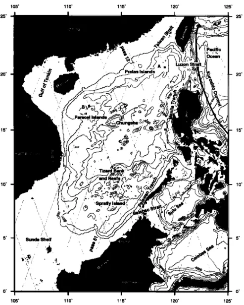
In recent years dic South China Sea (SCS) has attracted much attention from the oceanographic and geophysical communities. For example. scientists from east Asia, the United States, and Australia have joined the international project South China Sea Monsoon Experiment (SCSMEX) to study the water and energy cycles over SCS and its surrounding regions [Lau, 1997]. Figure I

Shaw and Chao's [1994] model also shows, among other features, a strong coastal current east of Vietnam, which is southward in summer and northward in winter. The model of Wu et al. [1998] indicates that interannual variation of the SCS velocity field are noticeable during El Nifio. Metzget and Hurlbutt [1996] modeled the coupled dynamics between SCS and the surrounding seas, concluding that the circulation interior to SCS is significantly affected by the wind curl field, especially the cyclonic gyre and

shows

the

major

surface

and

bottom

features

of SCS.

The SCS

is a the coastal

currents

off southern

China

and

Vietnam.

Metzger

and

semiclosed sea with major water exchanges occurring at the Tai-

wan Strait to the north, at the Luzon Strait to the east. and at the

Sunda Shelf to the south. Exchange of deep water can occur only at the Luzon Strait, where the water is sufficiently deep [Nitani, 1972]. According to the basic hydrodynamic equations [e.g., Apel, 1987, Chapter 3] the varying depths of 200 - 6000 m, the seamounts, the islands, the other shallow-water obstacles, and the monsoonal winds may well make the circulation and the eddy

Hurlbutt [1996] also show that the primary mechanism of the

seasonal inflow and outflow of water at the Luzon Strait is the

wind stress pileup from the monsoon. Furthermore, eddy observa- tions over SCS date back to the work of Dale [ 1956], who report- ed a cold-core eddy off east Vietnam in summer. The most recent in situ observation of the SCS eddies is due to Chu et al. [ 1998a], who discovered dual anticyclonic eddies in the central SCS basin and cyclonic eddies associated with the former. The mechanism of

fields

of SCS

very

complicated.

The observation

of the SCS

cir- the formation

of these

eddies

was

later

explained

by Chu

et al.

drifter observation of the SCS circulation is attributed to Hu

[1998], who reported seasonal variation of the SCS circulation. The numerical models of both Shaw and Chao [1994] and •t e! al. [1998] suggest that the SCS circulation is mostly wind-driven.

Copyright 2000 by the American Geophysical Union. Paper number 2000JC900092.

0148-0227/00/2000JC900092509.00

[1998b]. The first use of mixed remote sensing data for eddy detection over SCS was made by Soong et al. [1995], who discov- ered a cold-core eddy west of Luzon using TOPEX/Poseidon (T/P) altimetry, advanced very high resolution radiometer (AVHRR) temperature images, and drifter data. Later, Kuo and Ho [1998] discovered a cold-core eddy east of Vietnam using AVHRR, and they attributed this cold-core eddy to coastal upwelling. [ e.g., Grtidlingh, 1995; Meyers and Basu, 1999; Siegel et al., 1999]. Recently satellite altimetry has been increasingly used as a remote sensing tool to identify eddies.

23,944 HWANG AND CHEN: SOUTH CHINA SEA CIRCULATIONS AND EDDIES 25' 20' 15' 10' 105' 110' 115' 120' 125'

.?"

Luzon

Strait

f•) :'"-Spratly

Figure 1. Major surface

and bottom

features

and selected

contours

of depth

over the SCS. The letters

A and B

indicate

two crossovers

of T/P ground

tracks

(dots).

A number

near

a T/P track

is the pass

number.

Despite the huge effort in the past the existing observations of the SCS circulation and eddy field remain quite scattered com- pared to the size of SCS. This scattering makes it difficult to see the spatial and temporal evolution of circulation and eddy field over SCS, which are now largely based on numerical models. With the advent of satellite altimetry this sampling problem can be mitigated because altimetry can provide data of continuous cover- age in space and time. In particular, altimeter data are very useful for the study of time-varying circulation because there is no need of the geoid in this case [Wunsch and Stammer, 1998]. Interest- ingly, while the sea level of SCS has been extensively studied with satellite altimetry [e.g., Shaw et al., 1999; Hwang and Chen, 2000], the circulation and eddy field of the SCS have not received the same attention with altimetry; that satellite altimetry can be used to derive meaningful circulation and eddies in a marginal sea like SCS is not known with certainty. Accordingly, this study will focus on the derivations of the SCS circulation and eddy field using the best altimeter data to date: the T/P data, with an aim to discover phenomena not found in the existing observations and

result.

In the following

we first describe

the T/P data

processing,

then introduce methods to compute time-varying circulation and to locate eddies. T/P-derived circulation and eddies are then com-

pared with drifter velocities. Next, we show the T/P-derived cli-

matological

circulation

of SCS and the kinematic

properties

of

eddies and describe the characteristics of their seasonal and inter-

annual variations associated with El Nifio/Southern Oscillation

(ENSO).

We will use

NINO3 Sea Surface

Temperatures

(SSTs)

as

the index

of ENSO. As defined

by Kiladis

and Diaz [1989],

dur-

ing the time span of this study, i.e., from 1993 to 1999, there are three El Nifios, occuring in 1992-1993, 1994-1995, and 1997-1998, and one La Nifia, occuring in 1995-1996. Finally, we discuss the relationships between wind and some interesting phenomena and point out the possible causative mechanisms.

2. Data Processing

and Analysis Methods

2.1. T/P Altimeter Data Processing

T/P is an altimetry

mission

dedicated

to measuring

the ocean

HWANG AND CHEN' SOUTH CHINA SEA CIRCULATIONS AND EDDIES 23,945 20' 15' 10' 105' 110' I I \ ? 115' 120' I I

\

/

\ /

/

...•½;

,i . :...;ii

... ',,

I

i,,,

/',

,,

'i:

.... /

:.?:...

•?!.*'?,,; ...

::..i::;!:!::

)1(

•

,?.-,'"'

•..

...

d/': ',

,:.':,.,.•.

:.?•:•::

... '.;,.

...

,,.

..:*.

-,,,

--

. .:.•

•.•

•,-..,...

,.,

... • • '

,.

:..

....

..,..

.•4.,•

•.;

•,;,,...:...:½.,:•::.•

... ....

...

...

,

...

?..

.

...

???:' ?, ,

',,

I

\

:;/ ", :..?

... ß

..-,-,.-.%<,..¾

'"'•"•i4•••••••

'":'"'•

""

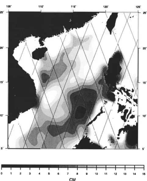
Figure 2. Sea surface height variabilities derived from 5.6 years of T/P altimeter data.

dented accuracy and nominal 10 day (actually 9.9156 days) repeat period, T/P is an important tool for deriving spatial and temporal variabilities of the ocean. In this study we used the T/P version C Geophysical Data Records (GDRs) from Archiving, Validation and Interpretation of Satellite Oceangraphic data (AVISO) [1996} to generate geophysically corrected sea surface heights (SSHs) from T/P cycle 10 (December 26, 1992) to cycle 219 (August 29, 1998). In particular, we have removed the ocean tide based on the CSR3.0 tide model [Eanes and Bettadpur, 1995]. The first nine

The variability is largest around the Luzon Strait, where water exchange between SCS and the Kuroshio Current occurs. In the areas east of Vietnam and west of Luzon the variability is also

relatively

large.

In general,

large

variability

occures

along

a band

across the SCS basin in the northeast-southwest direction. Nor-

mally, large SSH variability

is associated

with strong

circulation

and eddy activity, as will be demonstrated in section 3.

An important

issue

is whether

the tidal aliasing

contained

in

T/P data will affect the result in this paper.

The model error of

cycles

were

not used

because

of the mispointing

problem

[Fu et CSR3.0

over the SCS, especially

the tidal aliasing

problem,

has

al., 1994].

Other

details

of the T/P data

processing

were

described been analyzed

by Hwang and Chen [2000], who show that

by Hwang and Chen [2000], who used the same T/P data as those CSR.3.0 has the largest error over the continental shelf and the

used

in this study

to perform

Fourier

and wavelet

analyses

of the least

error

in the central

SCS basin.

Although

tidal model

error is a

SCS sea level. In fact, we have created

a T/P database

that re- complex

function

in space

and time, it can be reduced

by spatial

quires

only two simple

commands

to extract

SSHs

or sea level filtering

and temporal

averaging.

For example,

the three

longest

anomalies for any given area and cycles using the efficient algo- wavelengths of the aliasing M2 in T/P are 9 ø, 4.14 ø and 2.16 ø.

rithm

described

by Hwang

et al. [1998].

We also

averaged

SSHs Employing

the median

filter with a 300 km wavelength

on the

from the 210 T/P cycles (total 5.6 years) to yield along-track mean TP/SSHs, the 2.16 ø alias can be remove and the 4.14 ø alias can be

SSHs

for subsequent

analyses.

Figure

2 shows

the SSH variability reduced

substantially.

The 9 ø alias has a spatial

scale

that is too

over SCS derived

from this averaging

process

The anomalous

large

to affect

the results

presented

in this

paper.

The median

filter,

variability

over

the continental

shelf

is mainly

due to the aliasing which

will be used

by outliers

[Naess

and Bruland,

1989];

outliers

23,946 HWANG AND CHEN: SOUTH CHINA SEA CIRCULATIONS AND EDDIES

the SCS is frequently visited by violent typhoons. The choice of 300 km is based on the cross-track spacing of T/P (2.83 ø) and the requirement that the detail of SSH be retained while removing false signals. Also, as shown by Hwang [ 1997, Table 5], at a given

location a 10 cm M2 model error in T/Pcan be reduced to 2.26 and

0.41cm by averaging T/P data over 3months and 1 year, respec- tively. Nevertheless, because of the large tidal model errors over the continental shelf of the SCS including the Sunda Shelf, we ignore any result there in this paper. Another issue is whether the T/P data noise will produce false signals. To investigate this, we produced a smooth dynamic topography field by subtracting the Earth Gravitational Model 1996 (EGM96) geoid [Lemoine et al.. 1998] from the 5.6 year averaged SSHs (see section 2.2.1 for the definition of dynamic topography). We then added random noises to the dynamic topography based on a 4.7 cm standard error [Fu et al., 1994]. Finally, We used the median filter to smooth the origi- nal and the noise-disturbed dynamic topography fields. Contour plots of two smoothed dynamic topography fields show that they are almost identical (the plots are not shown because of limited space), and this similarity suggests that the T/P noises can be effectively eliminated by the median filter. Other evidence in the following development will also show that the T/P tidal aliasing and noise will not affect the result in this paper.

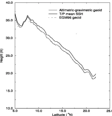
40.0 35.0 30.0 • 25.0 ._c• 20.0 15.0 Altimetric-gravimetric geoid T/P mean SSH ß 10.0 ' • ' • • 5.0 10.0 15.0 20.0 Latitude (øN) 2• ;.o

Figure 3. Comparison

of altimetric-gravimetric

geoid, EGM96

geoid, and T/P mean SSH along T/P pass 51. 2.2. Analysis Methods

2.2.1. Computing geostrophic velocity on a grid. In this case the dynamic heights from altimetry are first interpolated on a grid; then the horizontal components of geostrophic velocity are com- puted by [Ape/, 1987]:

g a( g a( g

• ... ½ (•)

f Rc3½ f 63y f

(2)

where (is the dynamic height; u and v are the east and north ve-

locity components,

respectively;

g is gravity,

f-2•2sin½,

from altimetry.

Replacing

(by ,4( (in reality,

,4h, the sea level

anomaly)

in (1) and

(2), one obtains

the relative

geostrophic

ve-

locity.

It is noted

that the T/P mean

SSHs

averaged

over 210 cy-

cles are rather close to some existing geoids over SCS and have accuracies better than 1 cm. As an example, Figure 3 compares the

T/P mean

SSH, the altimetric-gravimetric

geoid

of Hwang [1996]

and the geoid from the EGM96 gravity model to degree 360

[Lemoine

et al., 1998] along

T/P pass

51 (see Figure 1). Apart

from a constant bias, the first two agree quite well. Note that since

the goal of this study

is to derive

the time-varying

circulation

and

eddies

from T/P, relative

dynamic

height

will be always

used,

and

the computed

velocities

in this paper

are always

the relative

(time-

varying) geostrophic velocities. The word "relative" will be omit-

with•2

being

the earth's

rotational

rate

(7.292115x10

-s rad

s~•);

R ted in the following

development.

Furthermore.

on the basis

of

is the

mean

radius

of the

Earth,

• and /• are

the

latitude

and EGM96

dynamic

topography

model

[Lemoine

et al., 1998]

the

longitude;

and

x and

y are

the

local

rectangular

coordinates,

with mean

circulation

of SCS

is very

small

compared

to the clima-

positive

x to the east

and positive

y to the north.

The dynamic tological

circulation.

Thus,

in most areas

of SCS the relative

height

is the

difference

between

SSH,

h, and

the

geoidal

height,

N: geostrophic

flow

derived

with

A(will closely

resemble

the

abso-

(=h-N. (3)

The problem

with this approach

is that an accurate

geoid

over

the

oceans

is difficult

to compute.

Currently,

there

exist

geoid

models

over SCS, for example,

the model

of Hwang

[1996],

but the accu-

racies of these models may not be sufficient to resolve circulation

and

eddy

at the mesoscale

level.

However,

if we are only interest-

ed in the time-varying

circulation,

we need

only

the relative

dy-

namic

height

[Wunsch

and Stammer,

1998]

A(=(-(0 =h-h0 =Ah, (4)

where

•, is the time-independent

dynamic

height

and

h and

ho

are

the instantaneous

(after

removing

the tidal effect)

and mean

SSH

lute geostrophic

flow derived

with (, except

near

the Luzon

Strait,

where water exchange between SCS and the Pacific occurs and the Kuroshio Current will contribute a significant mean flow.

In the actual

computations

of time-varying

geostrophic

circu-

lation,

for each

T/P cycle

we first found

the median

dynamic

heights in 1 o x 1 o boxes, which were then used to construct a

I o x 1 o grid using

the minimum

curvature

interpolating

scheme

with a tension

factor

of 1 (a tension

factor

of 1 will make

the grid

as smooth

as possible)

[Smith

and Wessel,

1990].

Contour

plots

of

such

grids

show

many

unrealistic

signatures;

thus

at the final

stage

we employed

the median

filter with a 300 km wavelength

to

smooth

the 1 øx 1 o grid. At each

of the grid points

we evaluated

the

coefficients

of a quadratic

polynomial

that best

fits the dynamic

heights

around

this

grid

point.

Then

the first

derivatives

along

the

HWANG AND CHEN: SOUTH CHINA SEA CIRCULATIONS AND EDDIES 23,947

Descending North

Ascending

pass

a

pass

East

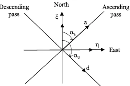
Figure

4. Ascending

(a), descending

(d), north

(x), and east

(h) components

of gradient

of the dynamic

height

at a

crossover of two ground tracks.

east and north directions were obtained from the quadratic poly- nomial and used to derive the velocity components by (1) and (2). For each cycle the times associated with all gridded velocities are the same and are the central time of this cycle.

2.2.2. Computing pointwise velocity at a crossover. In this case we are interested in the velocity components at a single point. It tums out that such a pointwise computation is possible only at the crossover of an ascending track and a descending track. Refer-

ring to Figure

4, the gradients

of the dynamic

heights

along

the

ascending and descending tracks, a and d, are [Heiskanen and Moritz, 1985, p. 187)

a=•: cosa, + r/sina, (5)

d = •: cosa a + r/sin a a (6)

where r/and •: are the east

and north

components

of gradient

(see

(1) and (2)), respectively, and ao and aa are the azimuths of the

ascending

track

and the descending

track

at the crossover,

respec-

tively. Inverting (5) and (6) leads to

COS O• d -- d cos a,

(,7) sin(a, - a a )

-a sin a a + d sin a,

• = , (8)

sin(a, - a a )

which can be used to derive velocity components by (1) and (2). The along-track gradients of the dynamic height can be computed by numerical differentiation, as was used in deriving the along- track deflections of the vertical [Hwang et al., 1998]. Gradients derived in this way will contain negligibly long wavelength effects because of orbit error and low-frequency tidal model error [Hwang, 1997]. Using this method, T/P is like a current meter that measures the geostrophic velocity at a crossover every 10 days. This method can be used to identify the type of an.. eddy and com- pute its velocity if a T/P (or any T/P class altimeter) crossover is located inside the eddy. For example, the crossover of T/P passes

12 and 51 is located to the west of Luzon (see Figure 1), so here one can compute the eddy velocity of the cold-core eddy discov- ered by Soong et al. [1995], who simply computed the velocity components perpendicular to passes 12 and 51 at selected spots.

However, this crossover method requires very accurate dy- namic height. To see this, we can derive the 1 cr errors of the east and north velocity components from (1), (2), (7), and (8) using error propagation:

g x/si

n

2

2

or,, = (9)

f [sin(a,

- aa

) cr

g

g •/cOS2

Or5

a + COS

2 Or5

d

f isin(a"

-aa) Crg

,

(10)

where crg is the 1 cr error

of the gradient,

which

is the same

for

the ascending and the descending gradients. In deriving (9) and (10) we assume that the errors of velocities are solely from the gradient components (the errors of azimuths will also make con-

tribution

but are

neglected).

A rough

estimate

of Crg

is [Hwang

et

al., 1998]

O-g

=•cr h ,

(11)

s

where cr h is the 1 cr error of the dynamic height and s is the along-track sampling interval. Because of T/P's inclination angle of 66 ø, which yields a relatively inaccurate east component of gradient, the v component has a much larger error than that of the u component. Assuming a 1 cm error for the mean SSH (or the geoid, in the case of absolute velocity), a 4.7 cm error for one single T/P-measured SSH [Fu et al., 1994, Table 2], and s = 6.2

km, we have Crg

•10.9x10

-6 rad. With

this

crg value

we find

that

or,, • 160 cm s

-I and cry,

• 400 cm s

'1 at crossover

A and

or,,

•189 cm s

'1 and

cry,

• 410 cm s

-1 at crossover

B (see Figure

1).

Clearly, by this method, T/P can detect only very large geostrophic currents at the 6.2 km wavelength. However, the long wavelength

23,948 HWANG AND CHEN: SOUTH CHINA SEA CIRCULATIONS AND EDDIES

component of geostrophic current can be determined with an improved accuracy using filtered along-track dynamic heights.

2.2.3. Identifying eddy and computing its kinematic prop- erties. In this study the identifications of eddies implied in the T/P data will be based on the contour plots of the dynamic height and plots of circulation. This approach has been used by, for example, Gr•indlingh [ 1995], Siegel et al. [ 1999], and Crawford and Whit- ney [1999]. An automatic edge detector may be used to detect an eddy [e.g., Meyers and Basu, 1999], but the complex land-ocean geometry of SCS and the relatively poor T/P data quality over the SCS will require a further, very subjective judgment before one can decide whether a detected eddy is reasonable and acceptable. An eddy will create a circle-like shape in the contour plot of dy-

zero. This assumption is reasonable over a semiclosed sea like the SCS but may not be valid over areas with energetic flows like the

Kuroshio Current and the Gulf Stream. The nonlinear observation

equations in (13) and (14) can be linearized using Taylor's expan- sion to the first-order term, and the parameters can be estimated by the least squares method. Appendix A describes the detail of our least squares method. An eddy is considered existent and its kine- matic properties considered acceptable only if (1) the normal matrix ATA in (A6) is positive definite, (2) iterations in the least squares estimation converge, and (3) the sign of the computed vorticity matches the type of the eddy (positive for cold-core eddy and negative for warm-core eddy).

namic height, and the derived circulation will show a signature of 3. Results eddy (see also the plots of circulation below). Note that a propa-

gating wave or an aliasing tide will also create sea surface eleva- tions, but one whose contours are mostly noncircular and de- formed [see also Schlax and Chelton, 1994]. Considering the accuracy of T/P dynamic height, in this paper the edge of an eddy is defined to be the 5 cm contour of dynamic height counting from the center of the eddy [see also Gr•indlingh, 1995]. The center of an eddy is estimated using the contour plots and will be later re-

3.1. Verification

3.1.1. Comparison of velocities. We first verify the T/P- derived velocities and eddies before doing any analysis of such

results. To this end we obtained velocities measured with drifters

over the SCS. The drifter data were mostly collected by Hu [1998] and were edited by Hansen and Poulain [1996], and are available vised by the least squares method discussed below. The radius of at the World Ocean Circulation Experiment (WOCE) data center. the eddy is defined to be the averaged distance from the center to

the edge on a Mercator prqjection. The distortion of distance in the Mercator projection over the SCS is small because SCS is near the equator. The distortion is also very small compared to the uncertainty in position. To compute the kinematic property of an eddy, we adopt the models used by Okubo [1970], Kirwan et al. [1984] and Sanderson [1995]. First, in the local rectangular coor- dinate system, the velocity gradients of an eddy are

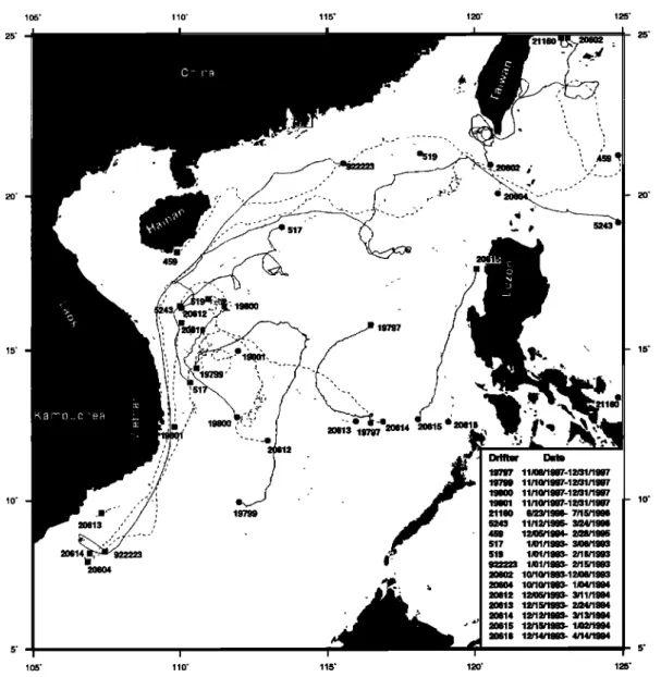
Hu [1998] also presented a preliminary analysis of the SCS circu- lation based on these drifters. Figure 5 shows the tracks of select-

ed drifters over the SCS, with some in the waters east of Taiwan

and the Philippines. These drifter data were collected during 1993- 1997. From Figure 5, in winter most of the drifters released at the Luzon Strait traveled in the anticlockwise direction and along the western boundary of the SCS. Drifter 20602 entered the SCS, circled off the shore of the southwestern Taiwan, and finally,

8u 8u 8v 8v

(12)

gl•-•xx,g•2

•y,g21 •xx,g22

8y

moved to the Pacific Ocean. Drifter 459 first circled around an

anticyclonic gyre east of Taiwan and then entered the SCS via the

Luzon Strait. Thus the tracks of drifter 20602 and 459 were indi-

where the definitions of u, v, x, and y are the same as those in (1) and (2) and g//, etc., are velocity gradients, which are assumed to be constants. The tbur kinematic properties to be computed are

cative of water exchange between the SCS and the Kuroshio Cur- rent as described by Shaw [1991 ]. The track of drifter 19801 indi- cates that an anticyclonic eddy existed east of Vietnam. The track vorticity = 2 x angular velocity = g2/-g/2,

divergence = g// +g22 , stretching deformation = g/z---g22 ,

shearing deformation = g2/+g/2.

In the Northern Hemisphere the vorticity is positive for a cyclonic eddy and is negative for an anticyclonic eddy. For a perfectly circular eddy with a uniform angular velocity, only the vorticity is nonzero. The vorticity can be interpreted as the fluid circulation per unit area. Given the T/P-derived velocities, the velocity gradi- ents and the coordinates of the eddy center, xo, Yo, can be estimated using the following model:

u(t)+e, -g,,[x(t)-Xo]+g,2[Y(t)-Yo]

(13)

v(t)+e,,

= g2,[x(t)-Xo]+g22[Y(t)-

yo] ,

(14)

where e,, and ev are the residuals of the observed u and v velocity components and t is the time of the observation. In this model we have assumed that the flow velocity of the eddy at the center is

of drifter 20616 shows a cyclonic eddy west of Luzon in January 1994, which was also detected by Soong et al. [1995] using this

same drifter and other data.

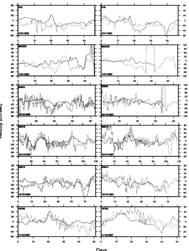
For comparison, the velocity components from T/P at the measuring times and locations of drifters were computed from the 10 day løxl ø dynamic height grids using three-dimensional poly- nomial interpolations in latitude, longitude, and time. (Because of the low spatial and temporal resolutions of the T/P velocities as compared to the drifter velocities, any reasonable interpolation methods will yield the same result in this case [see also Gerald and Wheatle•v, 1994, p. 274] for the expected error of polynomial interpolation. Figure 6 compares the T/P-derived and the meas- ured velocity components for six selected drifters of relatively long lifetimes. Excluding anomalous velocities and tidal currents, the temporal and spatial ranges of drifter velocities are roughly from 0 to 80 cms '1. It must be pointed out that, velocities meas- ured with a drifter contain geostrophic, inertial, tidal. and other currents [,4pel, 1987], while the T/P-derived velocities contain only the geostrophic component. In addition, the T/P-derived

HWANG AND CHEN' SOUTH CHINA SEA CIRCULATIONS AND EDDIES 23,949 105' 110' 115' 120' 125' ß

20'

.," :,,,/:•

... ...:.:..--_., :

517 '••_.• .

I /"; /

-,e20s14

5

ß

Figure

5. Tracks

of selected

drifters

from

the WOCE data

center.

Circles

and squares

indicates

the starting

and

ending

locations

of tracks.

Inserted

is a box showing

the starting

and

ending

times

of drifters

in the studied

area.

velocities are sampled at a 10 day interval, while the drifter ve- locities are sampled at a 6 hour interval. The T/P-derived velociti- es also have much lower spatial resolutions than those of drifter velocities because of the large cross-track spacing of T/P and the use of the median filter. From Figure 6 the T/P-derived velocities agree well with the drifter velocities at low frequencies. The over-

all directions of flow from T/P are consistent with those from the

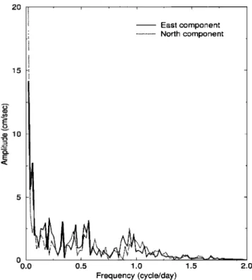
drifters. The T/P-derived velocities have the poorest fit, with the drifter velocities near the continental shelf of the SCS, where T/P data are less accurate and data gaps degrade the accuracy of inter- polation. The drifter velocities are highly oscillatory. As an exam- ple, Figure 7 shows the periodograms of the measured east and north components of velocity from drifter 19799, which traveled in the waters east of Vietnam. Figure 7 indicates that most of the high-frequency oscillations of drifter 19799 are at frequencies of 0.5 and I cycle day -l because of tidal currents.

3.1.2. Comparison of eddy kinematic properties. To see the comparison of eddy kinematic properties, we computed the kine- matic properties of the cold-core eddy west of Luzon from the

data of drifter 20616 and from the dynamic heights of T/P cycle 48 (mean time: January 7, 1994). The comparison is given in Table 1. In estimating the kinematic properties of this eddy we forced the center of the eddy determined from the drifter to be the center of the T/p-estimated eddy because the sparse drifter data have yielded large errors in the estimated eddy center. On the basis of Table I the vorticities and shearing deformations derived from the two data sets agree quite well, but the stretching deformations and divergences have large deviations, which are probably due to the different geographic distributions of drifter data and T/P data over this eddy.

3.2. Seasonal and Interannual Variations of the SCS Circulation

In the past, seasonal and interannual variations of the SCS circulation have been largely based on numerical models, for example, the models of Shaw and Chao [1994] and }Vu et al. [ 1998]. With satellite altimetry, for the first time we will be able to observe these variations. We have computed maps of the monthly

23,950 HWANG AND CHEN' SOUTH CHINA SEA CIRCULATIONS AND EDDIES 105' 110' 115' 120

20

cm/•

c 8/93

'

-,

., %i,:

••.

ß,..

%]

20'

i.

•..,•

.-

Plate 1. The relative

dynamic

heights

and the monthly

circulations

of the South

China Sea from August

1993 to

July 1994

derived

from

T/P ultimetry.

The months

and

years

are indicated

on the upper

left-hand

comers.

Monthly

HWANG AND CHEN' SOUTH CHINA SEA CIRCULATIONS AND EDDIES 23,951 105' 110' 115' I I I 120' 125' 105' 115' 120' 125' 105' ! I JUL 110' I I I FEB •, .... '"1'\" "''' MAR AUG JUN SEP 110' 115' 120' 125' I I i I 25' - ß

li •

"

ß

, ½,g-.-,//.--'-•,-:.:

•

116X..'t..:.->.

, '.r ,."

'

e,/../ " . . ' •

b.-,, :"..

)

,o-

23,952 HWANG AND CHEN: SOUTH CHINA SEA CIRCULATIONS AND EDDIES -40 -- 0 80 60 - 40 - 20 -- 0 -20 -40 - -60 - --8O

I I I I

s'm

s•9

I

I

I

I

60

_

.;

-20

•n• I • '-' I ": -' I

I I I •mn•

'

-•o

•222a

'"

22• I

I

,

•o

•i:t,;?;:j.',•

•:

,,;•:,,•

•

... ,,,, . ...

,,,

.'

'.,"L

,

•o _!"

"' '"'

'"

'

: ..

","

;'',.,";?

•

'"""

•

L

-,o

•o .o

_!•,.,:•,?,,

o

:«v

-..•.,,:_:..,,_••..•...,•:

• ," :/'%•

,,

•,•,i ... Z.• ' o

o 20 •o 60 •o •oo •o o •o •o 60 •o •oo •o

I I I I I I I I I I

80

•0•14

,•

•o -

!i:",:'

., . ,

,o

"'

,. !i

....

•o m•

I

I

I

I

I •

I

I ,

I

I

60

40

-- ,.,•,,,, ,,• " ' ["'

:',

... ':',"

-".. :,•"': ,t

•"

'•

'

--

40

'" " •' ""'"'

',/",,/,

: /

o

o -

•,,•

!• i•c .... /••-•

., ,, -

'

' !!";¾!,•,",•,'

¾'",

,,,,.

,',

',,,/,.'"

- -•o

-20

-

, • •

?.' ,

Days

Figure 6. Comparison of T/P-derived (solid lines) and drier-measured (dotted lines) velocities tbr six selected drifters: (left) The east component and (right) the north component. For each drifter the numbers are indicated in the upper left-hand corners, and the date of the first data points are indicated in the lower left-hand corners. Days are the elapsed days since the first data point.

namic topography values. As an example, Plate I shows the monthly circulations from August 1993 to July 1994. We also computed the 5 year averaged monthly circulation using

5 Ill --ns k = I t/s./ = 5 ,i = 1,...,I,j = 1,--.,J,m = 1,--.,12 (15) 5 Ill

Y'.

v,., (t,)

v,,•: t,=l

i=1--- l,j=l -.. J m:l --. 12 (16)

where i, j, k, and m are indices of longitude, latitude, year, and month, respectively, and I and J are the numbers of points in the longitudinal and latitudinal directions, respectively. The 5 year

HWANG AND CHEN: SOUTH CHINA SEA CIRCULATIONS AND EDDIES 23,953 20 15 0 o.0 East component ... North component 1.0 1.5 2.0 Frequency (cycle/day)

Figure 7. Periodograms of the velocities measured with drifter

19799.

averages

are given in Plate 2. Most of the large-scaled

features

in

Plate 1 and 2 agree

well with those

described

by Shaw and Chao

[1994]

and Wu

et aL [1998],

but T/P provides

much

better

spatial

and temporal

resolutions.

The directions

of currents

and the loca-

tions of eddies are consistent with those indicated by the tracks of the drifters in Figure 5. For example, the cyclonic eddy west of Luzon detected by drifter 20616 in January 1994 is clearly seen in Plate 1. Below is a summary of the seasonal and the interannual patterns of the SCS circulation based on Plate 1 and 2 and plots ol monthly circulations in other years (not shown here but available at http://space. cv. nctu.edu.tw).

3.2.1. Winter (December to February). In the northern SCS

and in the waters west of Luzon and east of Vietnam, there exist

cold-core, cyclonic eddies. In general, the overall direction of flow in winter is cyclonic. In particular, strong southward alongshore currents are present at the western boundary of the SCS, with the strongest ones occurring off Vietnam. In the early springs of 1995, 1997, and 1998 the eddies east of Vietnam were anticyclonic (warm-core), rather than cyclonic as in the early springs of 1994 and 1996. This early warming of the SCS water may be associated

with the 1994-1995 and the 1997-1998 E1 Nifios, At the Luzon

Strait the flows are mostly westward, suggesting that the water of

the Pacific Ocean enters the SCS in winter.

3.2.2. Spring (March to May). The SCS circulation is weak-

est in this season. In the northern SCS, there still exist cold-core

eddies. In the central and southern SCS, warm-core anticyclonic eddies start to emerge in March and become full-grown in May. This result confirms the discovery of a SCS warm pool in spring by Chu et al. [1997]. Furthermore, the dual anticyclonic eddies in the central SCS detected by Chu e! al. [1998a] in May 1995 can be seen in Plate 1. In fact, except in May 1996, which is a La Nifio year, such dual anticyclonic eddies were all present in Mays of the years under study. The alongshore currents at the western boundary of the SCS now have reversed direction to become northward, but the magnitudes are small compared to those in winter. The reversal of the direction of the alongshore currents is consistent with the result of the numerical model obtained by Shaw and Chao [1994]. In the spring of 1997 and 1998 the warm- core eddies were most energetic. At the Luzon Strait, there is now no clear indication of water exchange between the SCS and the

Pacific Ocean.

3.2.3. Summer (June to August). In this season the SCS circulation is largely anticyclonic. Evolving warm-core eddies can be found all over the SCS. East of Vietnam, except in 1995, a cold-core eddy begins to emerge in August. This cold-core eddy has been confirmed by Kuo and Ho [1998] using AVHRR tem- perature images. The northbound alongshore currents east of Viet- nam are very energetic in June and July but are weak in August. The alongshore currents turn eastward when reaching the northern boundary of the SCS. At the Luzon Strait the direction of flow now becomes eastward, suggesting that the SCS water enters the

Pacific Ocean in summer.

3.2.4. Autumn (September to November). This season marks the change of the circulation system of the SCS from the warm phase to the cold phase. The alongshore currents at the western boundary of the SCS weaken beginning in September and com- pletely reverse direction to become southward in November. In most years the cold-core eddy east of Vietnam formed in August continues to grow and becomes full-grown in November. Also, warm-core eddies are still present in the northern SCS. In general, the Pacific water begins to enter the SCS beginning in November via the Luzon Strait. For no obvious reason the dynamic topogra- phy in the autumn of 1996 was unusually high, and the cold-core eddy east of Vietnam virtually disappeared.

3.3. Variations of Circulation at Selected Spots

To supplement the results in Plate 1, we now select two im- portant satellite crossovers, one to the west of the Luzon Strait

Table 1. Comparison of the Kinematic Properties of Drifter-Implied and T/P-Derived Cold-Core Eddies West of Luzon Found in January 1994

Vorticity Shearing

Deformation Stretching

Deformation Divergence

T/P cycle 48 3.028__+ 0.195 0.301 __+ 0.195 0.808__+ 0.195 0.062-t- 0.195 Drifter 20616 2.770 __+ 0.383 0.366 __+ 0.383 1.373 __+ 0.383 -0.269 _ 0.383

23,954 HWANG AND CHEN: SOUTH CHINA SEA CIRCULATIONS AND EDDIES 8O 70 $o 50 40 3O 2o lO o -lO -20 -30 -40 -50 -6o -70 -80 60 50 40 30 2o lO o -lO -20 -30 -40 -50 -6o -7o -80

(a)• , i . .

(b) I

I , , I

I

, I

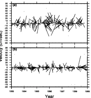
Figure 8. Stick diagrams of currents (a) at crossover A and (b) at crossover B. The locations of A and B are shown in Figure 1.

(crossover A) and the other to the east of Vietnam (crossover B), to see the seasonal and interannual patterns of circulation. The locations of A and B are shown in Figure 1. Figure 8 shows the stick diagrams of the T/P-derived currents at A and B computed with the crossover method. In the actual computations the along- track dynamic heights have been filtered by the Gaussian filter with a 100 km wavelength. We have experimented with many filter wavelengths, but the seasonal patterns can be seen only when the wavelengths of filter are > 100 km. Because our T/P data editing removes bad SSH observations, gaps exist in the two stick diagrams of Figure 8. From Figure 8a the direction of the current west of the Luzon Strait varies over the course of a year, but in general, the direction is mostly northeastward or eastward in spring and summer and is mostly southwestward or westward in winter. The change of the current direction is partly due to water exchange between the SCS and the Pacific Ocean around the Luzon Strait and partly due to the monsoonal wind stress [Metzger and Hurlburr, 1996]. In particular, from the spring of 1995 to the spring of 1996 the current west of the Luzon Strait has relatively large velocities. The T/P-derived current at B is rather noisy, probably because this location is near the continental shelf, where T/P has relatively poor data quality. However, from Figure 8b one still can see that the current at B is mostly southwestward or

westward in winter and is northeastward or eastward in summer.

The change of the current direction at B should be partly due to the monsoonal wind stress and partly due to the bottom topogra- phy (see section 4.2 for a detailed discussion). The result here demonstrates that T/P is an important tool for deriving pointwise

circulation, and the crossover method can be used to monitor

currents in other regions.

3.4. Kinematics anti Variation of Eddies

In Plate 1, we saw the spatial and temporal variability of cold- and warm-core eddies; now we will compute the locations of the

eddy centers and their kinematic properties. The eddies in Plate 1 are based on monthly averages, so eddies with lifetimes shorter than a month are not identified. In order to have a higher temporal resolution we use the original 10 day dynamic height grids to locate eddies. Because of data gaps and the use of the median filter, we will just compute the kinematic properties for eddies with radii larger than 150 km. As discussed in section 2.2.3, our edge detection of eddy is based on visual inspection of the 210 contour plots and the 210 circulation plots, and the kinematic properties are computed using the least squares method described in Appendix A. Figure 9 shows the distribution of eddies found using our method. In most cases a 10 day snapshot of the dynamic height from T/P contains more than one eddy. Although eddies may be found almost anywhere in the SCS (off the shelf), rela- tively high densities are found to the east of Vietnam, west of

Luzon, and east of the Paracel Islands. The eddies east of the

Paracel Islands and east of Vietnam are mostly warm-cored, while the eddies in the northern SCS are mostly cold-cored. The num-

bers of warm- and cold-core eddies west of Luzon are almost

identical. Furthermore, the distribution of eddies is found to be

sparse near the boundary of the SCS basin and near the shallow waters of the southern SCS. An eddy can easily change its shape, size, angular velocity, and other properties during the course of evolution, so many of the eddies in Figure 9 actually originated

from the same sources.

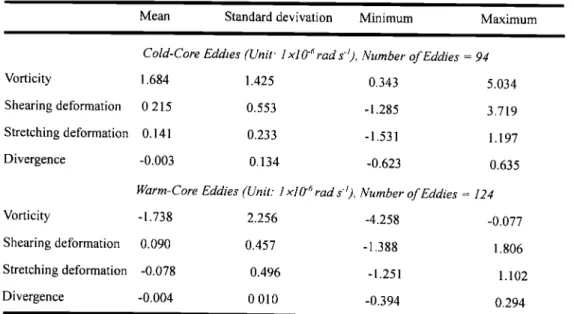
Table 2 shows the statistics of the kinematic properties of the eddies in Figure 9. From Table 2 the averaged vorticities of the cold-core and warm-core eddies are quite close. Both types of eddies have small divergences that are about one one thousandth of their vorticities. The shearing and stretching deformations of cold-core eddies are much larger than those of warm-core eddies, indicating that in general, the cold-core eddies are more deformed and noncircular. Because of the mathematical models used, the standard errors of the estimated vorticity, shearing and stretching deformations, and divergences are the same, and the averaged

standard

error

is 0.143

x 10

-6 rad s

-t. Also,

the averaged

standard

error of the estimated locations of the centers of eddies is 30 km.

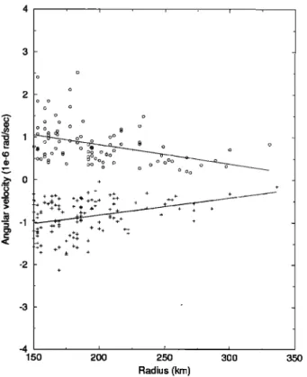
For both types of eddy the angular velocities are mostly < 1 x 10 '6

rads

-•, and

they have

no clear

dependence

on the radial

distances.

If we assume that the mean radius of the T/P-derived eddies is 250

km, then with a 1 x 10

'6 rad s

't angular

velocity

the tangential

velocity

is 25 cms

-• at the border

of the mean

eddy,

which

is about

the average of the tangential surface velocities of 10-40 cm s -• of the eddies discovered by Chu et al. [1998a]. Figure 10 shows the relationship between the radius and the angular velocity of an

eddy.

In general,

the smaller

the radius

of an eddy,

the larger

the

angular velocity. Assuming that a time-varying eddy has a con- stant mass, this radius-angular velocity relationship seems to con-

form to the law of energy

conservation.

Remarkably,

the slopes

of the radius-angular velocity relationship for the cold-core and warm-core eddies are almost the same and are --4x10 '9 rads '• km -•.

Figure 11 shows the monthly numbers of eddies for 1993-1999. In the winter of 1995-1996, which was during a La Nifia event, the

number

of cold-core

eddies

was relatively

large.

Normally,

warm-

core eddies

existed

only from spring

to summer,

but they existed

throughout most of 1997. In the summers of 1995 and 1998 the

numbers

of warm-core

eddies

were relatively

large.

Perhaps

the

most

interesting

phenomenon

about

eddies

is the presence

of both

HWANG

AND CHEN' SOUTH

CHINA SEA CIRCULATIONS

AND EDDIES

23,955

Figure

9. Distribution

of cold-core

eddies

(triangles)

and

warm-core

eddies

(squares).

cold-core and warm-core eddies in the waters east of Vietnam,

west of Luzon and west of Luzon Strait in different seasons of a

year. However, the times of the occurrences of these eddies and the way they evolved varied from year to year. As an example, Table 3 shows by year the occurring times of the first warm-core

and cold-core eddies east of Vietnam. The times in Table 3 were

obtained

by inspecting

all the eddies

found

in Figure

9 but focus-

ing on those near spring and summer. On the basis on Table 3, in 1997 and 1998 the warm-core eddies east of Vietnam occurred earlier in January, and in 1997 the cold-core eddy occurred much earlier than the average, August. If the mechanisms that create

these

eddies

have

to do with the monsoonal

winds,

then

the phase

Table 2. Statistics of Kinematic Properties of Eddies Over the South China Sea

Mean Standard devivation Minimum Maximum

Cold-Core

Eddies

(Unit.'

1 4 (• tad s-/),

Number

of Eddies

= 94

Vorticity 1.684 Shearing deformation 0.215 Stretching deformation 0.141 Divergence -0.003 1.425 0.343 5.034 0.553 -1.285 3.719 0.233 - 1.531 1.197 0.134 -0.623 0.635

Warm-Core

Eddies

(Unit.'

1 xl•T

• rad s-•),

Number

of Eddies

= 124

Vorticity -1.738 Shearing deformation 0.090 Stretching deformation -0.078 Divergence -0.004 2.256 -4.258 -0.077 0.457 -1.388 1.806 0.496 -1.251 1.102 0.010 -0.394 0.294