A CONSISTENT FINITE-ELEMENT FORMULATION FOR NONLINEAR DYNAMIC ANALYSIS OF PLANAR BEAM

IMERNATIONAL JOURNAL FOR NUMERICAL METHODS IN ENGINEERING, VOL. 37, 75-89 (1 994)

A CONSISTENT FINITE ELEMENT FORMULATION FOR

NON-LINEAR DYNAMIC ANALYSIS OF PLANAR BEAM

KUO MO HSIAO, RONG TSER YANG A N D AN W E N LEE

Department of Mechanical Enginem.ng, National Chiao Tung University, 1001 Tahsueh Road, Hsinchy Taiwan, Republic qf CUM

SUMMARY

A co-rotational finite element formulation for the dynamic analysis of planar Euler beam is presented. Both the internal nodal forces due to deformation and the inertia nodal forces are systematically derived by consistent linearization of the fully geometrically non-linear beam theory using the d'Almbert principle and the virtual work principle. Due to the consideration of the exact kinematics of Euler beam, some velocity coupling terms are obtained in the inertia nodal fonxs. An incremental-iterative method based on the Newmark direct integration method and the Newton-Raphson method is employed here for the solution of the non-linear dynamic equilibrium equations. Numerical examples are presented to investigate the effect of the velocity coupling terms on the dynamic response of the beam structures.

1. INTRODUCTION

In recent years, the non-linear dynamic behaviour of beam structures, e.g. framed structures, flexible mechanisms and robot arms, has

been

the subject of considerable research.'-13 Hsiao and Jan&' presented a co-rotational formulation and numerical procedure for the dynamic analysis of planar beam structures. In this formulation the Euler-Bernoulli hypothesis was employed and the unit extension of the centroid axis of the beam element was assumed to be constant. As extensively used in the literature, the inertia nodal force vector was obtained simply by the inner product of the mass matrix and the

nodal

acceleration vector.

This

formulation and numerical procedure were proven to be very effective by numerical examples studied in

Reference 11. However, the inertia

nodal

forces used

in

Reference 11 are derived from the linear beam theory. As mentioned in Reference 9, the use of linear beam theory cannot account for the complete inertia effects. In order to capture all inertia effects and coupling among extensional, flexural and torsional deformations for beam elements, the formulation of beam elements might be derived from the fully geometrically non-linear beam theory by consistent linearizati~n.~ Two consistent co-rotational formulations for three-dimensional beam element are proposed by Cri~field'~ and Hsiao," respectively. However, they are only limited for non-linear static analysis.

The objective of this study is to present a consistent formulation for the dynamic analysis of planar Euler beam in which the inertia

nodal

forces and

internal

nodal

forces due to deformation are systematically derived by consistent linearization of the fully geometrically non-linear beam theory using the d'Alembert principle and the virtual work principle. Here the Euler-Bernoulli hypothesis is properly considered.' Following Reference 1 1, the nodal co-ordinates, incremental displacements and rotations, velocities, accelerations and the equations of motion of the system are defined in terms of a fixed global co-ordinate system, while the total strains in the beam

0029-598 1/94/01OO75- 15$12.50

0

1994 by John Wiley &

Sons,

Ltd.

Received 1 September 1992 Revised 8 March 1993

76 K. M. HSIAO. R. T. YANG AND A. C. LEE

element are measured in element co-ordinates which are constructed at the current configuration

of the beam element. The element equations are constructed first in the element co-ordinate system and then transformed to the global co-ordinate system using standard procedure. The dominant factors in the geometrical non-linearities of beam structures are attributable to finite rotations, the strains remaining small. For a beam structure discretized by finite elements, this implies that the motion of the individual elements to a large extent will consist of rigid-body motion. If the rigid-body motion part is eliminated from the total displacements and the element size is properly chosen, the deformational part of the motion is always small relative to the local element axes; thus, in conjunction with the co-rotational formulation, the higher-order terms of nodal parameters in the element internal nodal forces and inertia nodal forces may be neglected. Due to the consideration of the exact kinematics of Euler beam, some velocity coupling terms are retained in the inertia nodal forces.

An incremental-iterative method based on the Newmark direct integration method and the Newton-Raphson method is employed here for the solution of the non-linear dynamic equilib- rium equations. Numerical examples are presented to investigate the effect of the velocity coupling terms on the dynamic response of the beam structures.

2. NON-LINEAR FORMULATION

2.1. Basic assumptions

The following assumptions are made in derivation

of

the non-linear behaviour: (1) The Euler-Bernoulli hypothesis is valid.

(2) The unit extension of the centroid axis of the beam element is uniform.

(3) The deformational displacements and rotations of the beam element are small. (4) The strain of the beam element is small.

The third assumption can always be satisfied if the element

size

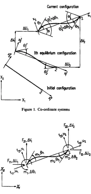
is properly chosen. Due to the assumption of small strain, the engineering strain and stress are used for the measure of the strain and stress. For convenience, the engineering strain is obtained from the corresponding Green strain in this study.

2.2. Co-ordinate systems systems (see Figure 1):

In order to describe the system, following Reference 11, we define two sets of co-ordinate

(1) A fixed global set of co-ordinates, X

, X2.

The nodal co-ordinates, incremental displace- ments and rotations, velocities, accelerations, and the equations

of

motion of the system are defined in this co-ordinate system.

(2) Element co-ordinates, x l , x2. A set of element co-ordinates associated with each element, which is constructed at the current configuration of the beam element. The element equations are constructed first in the element co-ordinate system and then transformed to the global co-ordinate system using standard procedure.

2.3. Nodal parameters and nodal forces

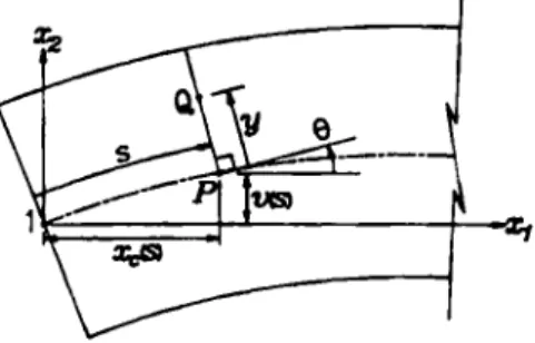
The element employed here has three degrees of freedom per node (Figure 2): these are the translations uj and v j ( j = 1,2) in the x1 and x2 directions, respectively, and the counterclockwise

A CONSISTENT FINITE ELEMENT FORMULATION 77

Current mfigurotion

"YIP*?

Figure 1. Cwrdinate systems

&.

AVz

Figure 2. Nodal parameters and nodal forces

rotations Oj ( j = 1,2) at nodes j. The nodal degrees

of

freedom for the global co-ordinate system are the incremental translations AUj and

Ac(

j = 1,2) in the X I and

X 2

directions, respectively, and the incremental counterclockwise rotations AOj ( j = 1, 2) at nodes j . The nodal forces corresponding to the nodal parameters are the conventional forces and moments as shown in Figure 2.

2.4. Kinematics of beam elements

The geometry of the beam element is described in the element co-ordinate system. In this study, the symbol { } denotes column matrix. Let

Q

(Figure3) be an arbitrary point in the beam

78 K M. HSIAO, R. T. YANG AND A C. LEE

Figure 3. Kinematics of the deformed beam

element, and P be the corresponding point of

Q

on the centroid axis. The position vector of point

P

in the undeformed and deformed configurations can be expressed as {xy 0) and {x,(s), o(s)),

respectively, where s is the arc length

of

the deformed centroid axis measured from node 1 to point

P . The relationship among x,(s), u(s), and s may be given as

where and x,(s) = u1

+

;

Sf,

cosedt 2s t = - l + -

S

(4)

in which u1 is the dispcement of node 1 in the x1 direction, 8 is t-e angle measured from the x1 axis to the tangent of the centroid axis and

S

is the current arc length of the centroid axis of the

beam

element. Note that due to the definition of the element co-ordinate system, the value of u1 is equal to zero. However, the variation and the time derivative of ul are not zero. Making use of equation (l), we obtain

where

and

G

= X,(S)

-

X,(O) = L

-

u1

+

u2

in which

L

is the length of the undefomcd beam axis and u2 is the displacement of node 2 in the

x1 direction.

The position vector of point

Q

in the undeformed and deformed configuration may be written as

A CONSISTENT FINITE ELEMENT FORMULATION 79

and

and displacement vector of point

Q

may be given by

r(s) = {x&)

-

ysin8, U(S)

+

ycose} ₍₉₎

u = r - r o (10)

If x and y are regarded as the independent variables, the Green strains E~~ (i = 1,2, j = 1,2) are given by

’

~ i j = *(GTGj

-

g:gj) (1 1) where and in which = (1

+

E 0 ) ( 1 . ar

h

as G , = - = -- ax asax

ar

G2

=

-

=

{

-sine, case} aY 1 E O = - - as

ax

ae

=

as

= CU” KY){COS 8, sin 8}

Note that K in equation (14) is an exact expression for the physical curvature of the deformed beam centroid axis. An equivalent expression of K

is

given

in

Reference 16.

Making

use of the

assumption of

uniform

unit extension, we m a y rewrite the unit extension e0 in equation (13) as

S E o = - - l

L (17)

Due to the

use of

the Euler-Bernoulli hypothesis, as expected, c l l is the only non-zero

(18) component of E ~ ~ . Substituting equation (12) into equation(l1) we may obtain

E l l = +C(1

+

Eo)2(1

-

KYI2

-

11

E = (1 -t h11)”’

-

1 = (1

+

h)(1

-

Ky) - 1

The engineering strain corresponding to e l l is

given

by”

(19) Note that E in equation (19) is an exact expression

of

engineering strain for the Euler

beam.

80 K. M. HSIAO, R. T. YANG AND A. C. LEE

Here, the lateral displacement of the centroid axis, u(s) is assumed to be the cubic Hermitian polynomials of

s

and is given by

u ( S ) = { N I , N t , N 3 , N4}T{V1, u ; , V2, u ; } = N i U b r (20)

where uj and v; (j = 1,2) are the nodal value

of

v and u‘ at nodes j, respectively.

N i

(i = 1-4) are shape functions and are given by

N ,

= i ( 1

-

5)2(2

+

t),

Nz

= i S ( l

-

r2)(1 - <)

(21)

N 3 = f ( 1

+

5)2(2

-

t),

N4 =

is(

-

1

+

< 2 ) ( 1

+

5 )

where S is the current arc length of the centroid axis, and

<

is the non-dimensional co-ordinate defined in equation (4).

2.5. Element internal nodal force vectors

The element internal nodal forces are obtained from the d‘Alembert principle and the virtual work principle. The virtual work principle requires that

SuXf,

+

buETfb = ( ~ E ~ C T

+

pbuTii) d V (22)

where

6ua = {bUl, 6UZ)

f b = f d , + f b = {fZl,mI,f22,m2} (26)

in which fg and

f j

( j = a, b) are the nodal force vector due to deformations and the inertia nodal force vector, respectively. b~ is the variation

of

E given in equation (19). CT = EE is the normal stress,

where E is the Young’s modulus. p is the density, 6u is the variation of u given

in

equation (10)

with respect to the nodal parameters, and ii = d2u/dt2. In this paper, the

symbol

(.) denotes differentiation with respect to time t , V is the volume of the undeformed beam.

The exact expression of

fa

and f b may be obtained by substituting the exact expression of 68, E,

bu, and u into equation (22). However, if the element size is properly chosen, the nodal parameters

of the element may always be much smaller than unity. Thus, only the first-order terms of

nodal

parameters are retained in

C

and f& and only zeroth-order terms of

nodal

parameters are retained in and p b . However, in order to include the effect of axial force, a second-order term of

nodal parameters is retained in

f”.

The approximations, 1

+

z 1, u’

=

8 and cos 8

=

1 are used in the derivation of fa and f b . In order to avoid improper omission in the derivation of fa and f b ,

these approximations are applied to the exact expression

of

b ~ , E, 6u and u.

From equations (2)-(7) and (14)-(17), the variation of E in equation (19) may be expressed as

(27)

bE

= (1 - Ky)bEo

-

(1 f E0)YbK where b K = CbU“

+

c3v’u”6t.’

6s

₂₆₆

_usfi

L fiL p L =

-

=

-

- -

A CONSISTENT FINITE ELEMENT FORMULATION 81

6d = {

-

1, 1}T{6~1, 6 ~ 2 ) = G f h ,

Sg

=

-

ct.'&'d<

1

I-

1

in which bu' and 6u" are the variations of u' and u", respectively, with respect to the nodal parameters. It should be noted that because the shape functions of u' and v'' are functions of S, the current arc length of the centroid axis, the variation of the shape functions are considered here. From equations (20), (21) and (28)-(31), the exact expression of 66 in equation (27) may be obtained. Using the approximations 1

+

e0 x 1, u' x 8 and cos 8 x 1, and retaining all zeroth- order terms and one first-order term of nodal parameters in the exact expression of &, we may obtain

(32)

1

1

BE

=

-

Gi6ua

+

1

u'NbTd< &I[

-

yNgTGu;

L 2 - 1

From equations (1)-(9), (20) and (21), the exact expression for 6u, the variation of u in equation (10) may be obtained. Using the approximations 1

+

.so 2 1, u' z 8 and cose x 1, and

retaining all zeroth-order terms of nodal parameters in the exact expression of

bu,

we may obtain

where

(33)

(34)

From equations (1)-(lo), (20) and (21), the exact expression of

u

may be obtained. Using the approximations 1

+

E~ x 1, u' 2 8 and cos 8 2 1, and retaining only zeroth-order terms of nodal

parameters in the exact expression

of

ii, we may obtain

where

and

(36) (37)

Note that i i and iii (i = a, b) are the absolute velocity and acceleration vectors of an element referred to the element co-ordinates which are obtained from the transformation of the corres- ponding global velocity and acceleration vectors extracted from the equations of motion of the system using standard procedure.'

Substituting equations (19), (32), (33) and (35) into equation (22), using the approximations 1

+

eo x 1, ur x 8 and cos 8

z

1, dropping higher-order terms of

nodal

parameters, and equating the terms on both sides of equation (22) corresponding to virtual displacement vectors

bu,

and

82 K. M. HSIAO. R. T. YANG AND A. C. LEE

6ut,

respectively, we may obtain

ft

= AEQG,

where A is the cross-sectional area and I =

j A

y 2 dA. The underlined terms in equations (41) and (42) are called the velocity coupling terms in this study. Note that if the velocity coupling terms in equations (41) and (42) are dropped, equations (39)-(42) are identical to the element nodal forces in Reference 1 1.

2.6. Element matrices

The element stiffness matrices and mass matrices may be obtained by differentiating the element nodal force vectors in equations (39)-(42) with respect to nodal parameters, and time derivatives of nodal parameters. However, element matrices are only used to obtain predictors and correctors for incremental solutions

of

non-linear equations in this study. Approximate element matrices can meet these requirements.

Thus,

the element matrices used in Reference 11 are adopted here for simplicity.

2.7. Equations of motion

The non-linear equations of motion may be expressed by

cp =

F'

+

F~

-

P

=

o

₍₄₃₎

where cp is the unbalanced force among the inertia force F', internal nodal force due to deformation

FD,

and the external nodal force

P.

F'

and

FD

are assembled from the element nodal force vectors in equations (39)-(42), which must be transformed from element co-ordinate system to global co-ordinate system before assemblage using standard procedure.

In this paper, an weighted Euclidean norm of the unbalanced force is employed for the equilibrium iterations, and is given by

where cp, is a reference unbalanced force, which is chosen to be the unbalanced force obtained at the first iteration in the present study; etol is a prescribed value of error tolerance.

83

A CONSlSTrNT FINITE ELEMENT FORMUUT'ION 3.

APPLICATIONS

An incremental iterative method based on the Newmark direct integration method ll.

''

and the

Newton-Raphson method is employed. The procedure used here to determine the deformational nodal rotations for individual elements is the same as that proposed in Reference 11 and is not repeated here.

In order to investigate the effect of the velocity coupling terms on the dynamic response, four examples are studied for the cases with and without consideration of the velocity coupling terms. It is found that for the first three examples the results obtained for both cases are nearly identical, but for the last example the discrepancies between the results obtained for both

cases

are not

negligible.

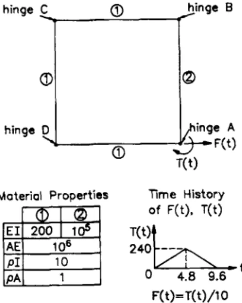
Material Properties Time History

of F(t), T(t)

EI 200 1

24$7A

/ t 4.8 9.6

F( t)=T( t)/l 0 Figure 4. Ryhg c l d - l o o p chain

\

/

\

\

t=4.8 t=9.6 t=14.4

I

/

84 K. M. HSIAO. R. T. YANG A N D k C. LEE

3.1, Flying closed-loop chain

The first example considered is a closed-loop chain'' constituted of four flexible

links

interconnected by hinges as shown in Figure4. The geometry and material properties of the closed-loop chain are also shown in Figure 4. Initially, the closed-loop chain forms a square of length 10 on each side. The whole system has no prescribed displacement boundary condition.

A force and torque are applied at end A

of

the

link

AB as shown in Figure 4. The closed-loop chain is discretized using

40

equal elements. The time step size is set to 001 and the error tolerance is set to

lo-'.

The entire sequence of motion is shown in Figure

5.

Also

shown

in

Figure

5

are the results reported in Reference 10. It is observed that the present results are in agreement with those in Reference 10.

3.2. Flexible robot arm with end rotation

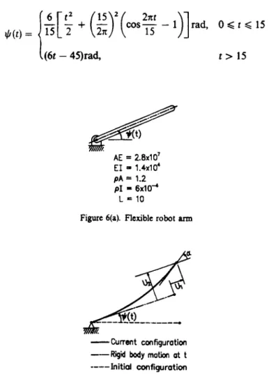
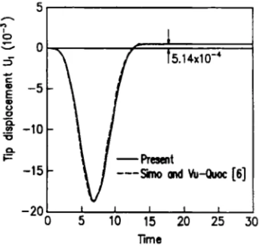
This example considered is a flexible beam rotating horizontally about a vertical axis passing through one end.6 Figure 6(a) shows the geometry of the beam and material properties. This beam is subjected to a prescribed rotation angle $(t) at one end as follows:

EI

-

1.4~10' pA = 1.2

PI = 6 ~ 1 0 ~ L = 10

Figure 6(a). Flexible robot arm

-Current configuration

----

Initial configuration --Rigid body m o t h ot t

A CONSISTENT FINITE ELEMENT FORMULATION 85

-20 I I I I I I

0 5 10 15 20 25 Z

rm

Figure 7(a). Time history for displaccment component U ,

I I I I I

0 5 10 15 20 25 30 -0.6

Time

Figure 7(b). Time history for displacement component U 2

1

-

_{$ 0} cI -1

-

-2 2 3 -3 0

F"

-4 .u v c 0 0

.-

c. E 0 oa -5 I I I I I 5 10 15 20 25 T i c

86 K. M. HSUO, R. T. YANG AND A. C. LEE

The beam is discretized using four elements. The time step size is set to 0005 and the error tolerance is set to lo-". The time histories of the tip displacements

U 1 ,

U 2 ,

and the tip rotation a, which are defined in Figure 7(b), are shown in Figures 7(a)-(c). Also shown in Figures 7(a)-(c) are the results reported in Reference 6. It is observed that the present results are in agreement with those in Reference 6.

3.3. Planar manipulator

The planar manipulator' shown in Figure 8 consists of two links. Two cases are considered: (a) both links are considered flexible and (b) link 1 is considered rigid. The geometry, inertia properties and material properties of the planar manipulator are given in Figure 8. For case (b), the Young's modulus of link 1 is set to lo4 times as large as that of link 2 to simulate rigid link.

Link

1 rotates with constant angular velocity o = 10 rad/s, while the motion of link 2 is such that its tangent at point A always remains in the horizontal position. This is assumed to be achieved by the joint moment. Weight of the bodies acts in the downward direction.

= t12 = 0. The initial elastic deformations are assumed to be zero, and the initial velocities and accelerations of the manipulator are calculated by using kinematics

of

rigid mechanism. Each member is discretized by four elements. The time step

size

is chosen to be 0.0013 s and the error tolerance is set to 10-l2.

Initially,

Lc = LZ = 0.8 m

A1 = Az = 0.0004 rnz

I, = 4 1 ~ = 5.333~10~ rn' m, = 4 = 2.512 kg Figure 8. Planar manipulator

-

Presmt

---

Ider and Amirouche [8]

-8'

A CONSISTENT FINITE ELEMENT FORMULATION ₈₇ The transverse tip deflections of link 2 measured from the tangent at point A are shown in Figures9(a) and 9(b) for both cases. Also shown in these figures are the results reported in Reference 8. It

is

seen that the agreement between these two solutions is very good.

3.4. Flexible robot arm with end torque

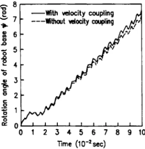
The flexible beam as shown in Figure 10 is subjected to an end torque. Initially,

4

= 0. The beam is discretized by ten elements. The time step size is chosen to be 00002 s and the error tolerance is set to lo-''.

The sequence of motion is depicted in Figure 11, and the time history of the rotation angle of the tangent at the robot base is shown in Figure 12. It is observed that the discrepancies between the results for the cases with and without the consideration of the velocity coupling terms are remarked.

4. CONCLUSIONS

This paper

has

described a consistent finite element formulation for the dynamic analysis of planar Euler beam in which the inertia nodal forces and internal nodal forces due to deformation are systematically derived by consistent linearization of the fully geometrically non-linear beam

-

Present

---

Ider and Amirouche

[a]

-81

Figure 9(b). Tip deflection of link 2 (link 1 rigid)

E = 2x1 0" N / d p = 7860 k g / ~ L = l m

A=4x104 m2

t(sec) I = 1 . 3 3 3 ~ 1 0 ~ m4 Figure 10. Flexible robot a m with end torque

88 K. M. HSIAO. R. T. YANG AND A. C. LEE

0.032 0.024

I:

-

With velocity coupling

----

Without velocity coupling

Figure 11. Sequence of motion for flexible robot arm

c

0

0 1 2 3 4 5 6 7 8 9 Time (tO-*sec)

3

Figure 12. Time history for rotation angle of the tangent at robot base

theory using the d'Alembert principle and the virtual work principle. In conjunction with the co-rotational formulation, the higher-order terms

of

nodal parameters in element nodal forces are consistently neglected. Due to the consideration of the exact kinematics of the Euler bearn, some velocity coupling terms are obtained in the inertia nodal forces. From the numerical examples studied, it is found that the effects of these velocity coupling terms on the dynamic response are remarked for some cases.

Although not included in the present derivation, the inclusion of damping forces presents no difficulties. It is believed that the consistent co-rotational formulation for

beam

element presented here may represent a valuable engineering tool for the dynamic analysis of planar beam structures.

A CONSISTENT FlNlTE ELEMENT FORMULATION 89

ACKNOWLEDGEMENT

The authors would like to acknowledge the constructive and thoughtful comments of the referees. The research was sponsored by the National Science Council, Republic

of

China, under the contract

NSC79-0401409-15.

REFERENCES

1. K.-J. Bathe and E. Ramm, ‘Finite element formulations for large deformation dynamic analysis’, 1nt.j. nwner. methods 2 C. Oran and K. Kassimali, ‘Large deformations of framed structures under static and dynamic loads’, Comput. Strut.,

3. D. P. Mondkar and G. H. Powell, ‘Finite element analysis of non-linear static and dynamic response’, Int. j. muner.

4. S. N. Remseth, ‘Nonlinear static and dynamic analysis of framed structum’, Comput. Smct, 10, 879-897 (1979). 5. T. Y. Yang and S. S a i d ‘A simpk ekmcnt for static and dynamic response of beams with material and geometric 6. J. C. Simo and L. Vu-Quoc, ‘On the dynamics of flexible teams under large overall motions-the planar case: Part I

7. T. R. Kane, R. R. Ryan and A K. Bane+, ‘Dynamics of a cantilever beam attached to a moving base’, J. Guidnnce 8. S . K. Ider and F. M. L. Amirouche, ‘Nonlinear modeling of flexible multibody systems dynamics subjected to variable 9. J. C. Simo and L. Vu-Quoc, ‘The role of non-linear theories in transient dynamic analysis of flexible structures’, 10. L. Vu-Quoc and J. C. Simo, ‘Dynamics of earth-orbiting flexible satellites with multibody components’. J. Guidance 11. K. M. Hsiao and J. Y. Jan& ‘Nonlinear dynamic analysis of elastic frames’, Comput. Struct, 33, 1057-1063 (1989). 12 Z Yang and J. P. Sadler, ‘Large-displacement finite element analysis of flexible linkages’, J. Mech. Design ASME, 112, 13. A K. Banerjce and M. E. Lemak. ‘Multi-flexible body dynamics capturing motion-induced stiffness’, J. Appl. M e c h 14. M. A. Crisfield, ‘A consistent co-rotational formulation for non-linear, three-dimensional, beamzlements’, Comput. 15. K. M. Hsiao, ‘Cororational total Lagrangian formulation for three-dimensional beam element’, AIAA J, 30,797-804 16. D. H. Hodges, ‘Proper definition of curvature in nonlinear kam kinematics’, A I A A J., 22, 1825-1827 (1983). 17. T. J. Chung, Continuum Mechanics, Rentice-Hall, bgkwood cliffs, NJ., 1988.

18. K. J. Bathe, Finite Elerncnf Procedures in Enginmhg Analysis, Rentice-Hall, E n g l e w d cliffs, NJ, 1982 eng, 9,353-386 (1975).

6, 539-547 (1976).

methods eng., 11,499-520 (1977).

nonlincaritia’, Int. j. muner. methods eng.. 20, 851-867 (1984). and Part II’, 1. Appl. Mech. ASME, 53, 849-863 (1986). Control Dyn., 10, 139-151 (1987).

constraints’, J. Appl. M e c h ASME, 56, 444-450 (1989). J. Sound Vib, 119,487-508 (1987).

Control Dyn, 10, 549-558 (1987).

175-182 (1990).

ASME, 58, 766-775 (1991).

Methods AppL M e c h Eng, 81, 131-150 (1990). (1992).