針對無線感測器網路的訊息中繼考慮通道參數不匹配的低冗餘波束形成設計

國

立

交

通

大

學

電信工程研究所

碩

士

論

文

針對無線感測器網路的訊息中繼考慮通道參數不匹配的低冗

餘波束形成設計

Low-Overhead Cooperative Beamforming for Information

Relaying in Wireless Sensor Networks Under Mismatched

Inter-Node Link CSI

研 究 生：胡仲萱

指導教授：吳卓諭

針對無線感測器網路的訊息中繼考慮通道參數不匹配的低冗

餘波束形成設計

Low-Overhead Cooperative Beamforming for Information

Relaying in Wireless Sensor Networks Under Mismatched

Inter-Node Link CSI

 

研  究  生：胡仲萱      Student：Chung-Hsuan Hu 

指導教授：吳卓諭      Advisor： Jwo-Yuh Wu 

 

國  立  交  通  大  學 

電信工程研究所 

碩  士  論  文 

A Thesis

Submitted to Institute of Communications Engineering National Chiao Tung University

in Partial Fulfillment of the Requirements for the Degree of

Mas1ter of Science in

Communications Engineering June 2012

Hsinchu, Taiwan, Republic of China

摘要

於低訊號冗餘合作式通訊系統中的高效能訊號處理演算法在實現節能的第四 代中繼網路中扮演著重要的角色。在這篇論文中，我們研究在無線感測器網路中 針對訊息中繼來考慮在通道參數不匹配的情況下的低冗餘合作式波束形成設計。 在我們所考慮的系統中，為了達到降低傳送通道狀態資訊的訊號冗餘，每一個中 繼端會將其測得之訊源與中繼端的鏈結訊雜比量化成一位元的訊息。為了反映無 線感測器網路嚴格的傳送功率限制，每一個訊雜比的量化訊息在傳輸過程中因此 假設為不理想的，於數學上視為經由一個帶有非零交叉機率的二元對稱通道來傳 送。當接收端接收這些可能有位元翻轉的一位元訊雜比訊息，且假設中繼端與接 收端間鏈結的通道估測是完美的，則我們首先可以考慮藉由最大化接收訊號的訊 雜比期望值所得的波束形成系數設計，其中此訊雜比公式是針對二元對稱通道中 位元翻轉的統計特性所求得的期望值。接著，我們進一步延伸考慮中繼端與接收 端間鏈結的通道估測可能會產生誤差的情況，在數學上我們以獨立同分佈的高斯 隨機變數才表示。在這兩種情況下，我們可以透過針對訊雜比不確定性或是通道 狀態資訊不確定性作平均，以分別推導出具封閉形式的條件平均接收訊雜比。因 為如此推導出來的訊雜比公式對波束形成系數來說是一高度非線性函數，所以針 對這兩種訊雜比公式，我們分別進一步地推導出各自的可分析下界以利於分析。 藉由最大化各自的訊雜比下界，相應的亞最佳波束形成系數解即可透過解廣義特 徵值問題來求得。最後，電腦模擬結果用以檢驗我們提出方法的成效。

Abstract

   

High-performance signal processing algorithms for cooperative communication systems with reduced signaling overhead play a key role toward realizing energy-efficient relay networks for 4G and beyond. In this thesis, we study the problem of low-overhead cooperative beamforming design for information relaying in wireless sensor networks (WSNs) by taking account of the effect of mismatched inter-node channel state information (CSI). In the considered system, each relay node quantizes the signal-to-noise ratio (SNR) of the source-to-relay (S-R) link into one bit in order to reduce the signaling overhead dedicated to CSI transmission. To reflect the severe transmit power limitation of WSNs, the transmission link of the quantized SNR message is assumed to be non-ideal, and is modeled by a binary symmetric channel (BSC) with a non-zero crossover probability. With the flipped one-bit SNR messages received at the destination and assuming that the relay-to-destination (R-D) link channel estimation is perfect, we first study the beamforming design based on maximization of the expected receive SNR, averaged with respect to the bit-flipping distributions of BSC's. Next, the proposed approach is extended to the scenario wherein the R-D link channel estimation errors occur, and are modeled as i.i.d. Gaussian random variables. In both cases, we derive closed-form expressions for the conditional receive SNR averaged over the distributions of the SNR/CSI uncertainty. Since the SNR measures thus obtained are highly nonlinear functions of the beamforming coefficients, we further derive for each case a tractable SNR lower bound to facilitate analyses. By conducting maximization with respect to the derived SNR lower bounds, suboptimal beamformers can be obtained via solving generalized eigenvalue problems. Computer simulations are used to illustrate the performances of the proposed schemes.

Acknowledgement

  兩年的研究所生涯即將結束，能夠順利完成學業及論文，首先要感謝的是我 的指導教授吳卓諭老師。不管是在學術領域上的指導抑或是為人處世的態度，都 讓我在這兩年研究所生涯中受益良多。他讓我了解到想要做好研究，必須要有認 真的態度和嚴謹的邏輯思考。感謝老師提供了舒適的研究環境及豐富的研究資源， 讓學生能夠毫無後顧之憂的進行學習及研究。在此，我要向吳卓諭老師獻上最誠 摯的感謝。 感謝所有在我研究所生涯中，陪我度過一次次不論是困難挫折、或是歡笑淚 水的校園同儕、朋友們。有你們的相伴，才有一路走來日漸茁壯的我。 最後，我要感謝我的父母，謝謝你們一路上支持我、鼓勵我，並且在人生的 抉擇中，給予我諸多建議，讓我能夠順利的走到現在。僅以此論文獻給我所有親 愛的家人。                              

Contents

    Mandrain Abstract i English Abstract ii Acknowledgement iii Contents iv List of Figures v 1 Introduction 1 1.1 Overview………...1 1.2 Contribution………...2 1.3 Organization………..3

2 System Model and Overview of Previous Work 5

3 Beamforming Design in the Presence of Imperfect Quantized S-R Link SNR 9

3.1 Conditional Average SNR……….9

3.2 Closed-Form Suboptimal Solution………..12

3.3 Simulation Results ……….13

4Beamforming Design Under Imperfect Quantized S-R Link SNR and R-D Link Channel Estimation Errors 17

4.1 Exact Formula for the Conditional Average SNR………...18

4.2 Approximation for the Conditional Average SNR………..21

4.3 Design of Beamforming Weights………23

4.4 Simulation Results………...24 

Conclusion 30

Appendix 31

References 51

List of Figures

1

(a) Low-overhead cooperative beamforming system diagram; (b) Depiction of AF relay and S-R link SNR quantizer………...8

2

Simulated BER of the proposed beamformer (3.17) and the solution in [10]… …..15

3

BER results of two methods with respect to different crossover probabilities……..16

4

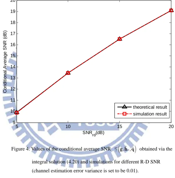
Values of the conditional average SNR ( ,g g h q  obtained via the integral r, )

solution (4.20) and simulations for different R-D SNR (channel estimation error variance is set to be 0.01)………..………26

5

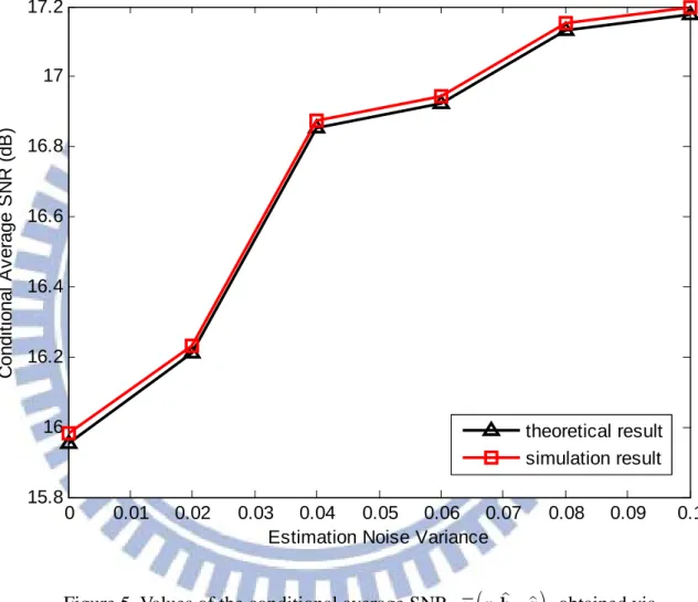
Values of the conditional average SNR ( ,g g h q  obtained via the integral r, )

solution (4.20) and simulations for different channel estimation error variance (R-D SNR is set to be 15 dB)……….………27

6

BER performance of the proposed beamformer (4.32) and the two solutions in [10]

and (3.17) for different R-D SNR………..28

7

BER performance of the proposed beamformer (4.32) and the two solutions in [10]

and (3.17) for different channel estimation error variance………29

8

BER results for two methods when 2-bit SNR quantization is adopted at each

Chapter 1

 

Introduction

 

 

1.1 Overview

Due to the myriad real-world applications, the study of wireless sensor networks, in particular, the development of high-performance distributed signal processing algorithms, has received considerable attention in the recent years [1-6]. Typically, sensor nodes are of a small size, powered by battery, and therefore subject to limited communication and message processing capability. Under such constraints, cooperation among sensors for information relaying or data forwarding becomes necessary in order to enable various global target tasks, e.g., data aggregation, decision fusion, and signal retrieval. Among the various cooperative transmission schemes, cooperative beamforming is a promising technique capable of realizing distributed spatial diversity toward link reliability enhancement [7-10]. Since the design of beamforming coefficients requires the knowledge of the channel state information (CSI) of inter-node channel links, communication/signaling overheads dedicated to CSI transmission, or feedback, in cooperative beamforming systems are thus unavoidable. To meet the high energy-efficiency demand for wireless sensor networks, the reduction of physical-layer signaling overhead is crucial [11-16]. There have been many studies of low-overhead cooperative beamforming techniques aimed at realizing energy-efficient information relaying, e.g., see [17-20]. In all of these works, it is commonly assumed that CSI transmission and feedback are errorless. Such an assumption, however, is impractical in the sensor network scenario. Indeed, since sensor nodes are subject to stringent power and decoding complexity constraints, implementation of forward error correction codes for improving the error resilience of quantized CSI (or information bits) may be prohibitive due to unacceptable system complexity and decoding latency [1, Chap. 6]. As a result, the transmission of the local CSI from the far-end relay nodes could be deteriorated by large path loss and severe fading, resulting in distorted CSI received at the destination. In point-to-point multi-antenna communications with limited feedback,

system designs in the presence of CSI transmission/feedback errors have been well documented, see, e.g., [21-25]. Related study in the context of cooperative communications, however, remains much to be investigated.

1.2 Contribution

In this thesis, we study the cooperative beamforming design for information relaying in wireless sensor networks in the presence of mismatched inter-node CSI. The cooperative beamforming scheme employing the amplify-and-forward (AF) relaying protocol as in [10] is considered. Also following [10], the information symbols are assumed to be BPSK modulated so as to reflect the rate and decoding complexity/latency constraints in wireless sensor networks [1], [6]. The design of the beamforming weights is aimed at maximizing a certain signal-to-noise ratio (SNR) metric at the destination. To reduce the signaling overhead, each relay node quantizes the SNR of the source-to-relay (S-R) link into one bit1, which is then sent to the destination for beamforming design. Rather than assuming that the quantized SNR messages are received at the destination without errors, we consider the realistic case that the transmission link of the one-bit message is imperfect, and is mathematically modeled as a binary symmetric channel (BSC) with a known crossover probability2. Specific technical contributions of this thesis can be summarized as follows.

(I) Beamforming Design in the Presence of Imperfect Quantized S-R Link SNR

We first consider the beamforming design by taking account of the fact that each one-bit message of S-R link SNR could be flipped by the BSC, while the R-D link channel estimation is assumed to be perfect. Given the one-bit messages received from all relays, the beamforming coefficients are designed at the destination via

1. While multiple-bit quantization at relays is considered in the problem formulation in [10], the simulation study

therein shows that the beamformer designed based on even one-bit quantization can perform quite close to that

designed in accordance with the full S-R link CSI. Hence, to minimize the signaling overhead, this paper focuses

on the specific one-bit case. The generalization of our current solution to the multiple-bit case is under

investigation.

maximization of the receive SNR averaged with respect to the conditional bit flipping distributions of BSC’s. A closed-form formula for the proposed SNR metric is first derived. The formula is seen to be a highly nonlinear function of the beamforming factors, and direct maximization of this objective function is quite difficult. For analytic tractability, we then derive a lower bound of the conditional average SNR that admits the form of a generalized Rayleigh quotient [26]. By conducting maximization with respect to this lower bound, a closed-form suboptimal beamformer can be obtained as the solution to a generalized eigenvalue problem. Computer simulation shows that the proposed scheme does outperform the solution [10] under imperfect quantized S-R link SNR.

(II) Beamforming Design Under Imperfect Quantized S-R Link SNR and R-D Link Channel Estimation Errors

Next, we generalize the results in part (I) by further taking into account the effect of R-D link channel estimation errors. It is assumed that the destination only knows a set of R-D link channel estimates, which are modeled as the true channel gains corrupted with additive white Gaussian errors. Conditioned on the received one-bit quantized S-R link SNR from all relays and estimated R-D link channel parameters, the design criterion of the beamformers is to maximize the receive SNR (at the destination) averaged over the distributions of both the bit-flipping effect of BSC's and R-D link channel estimation errors. An exact formula of the adopted conditional average SNR is first derived. Since the formula is quite complicated, to ease analysis we further resort to certain approximation techniques to derive an associated SNR lower bound which also admits the form of a generalized Rayleigh quotient [26]. As in part (I), we propose to instead conduct maximization of this lower bound. A suboptimal beamformer can be obtained as the solution to a generalized eigenvector problem. Computer simulations show that, compared to the beamformer [10] and the solution derived in part (I), the proposed design is more robust against the R-D link channel estimation errors.

1.3 Organization

introduces the system model and the problem statement. Chapter 3 presents the beamforming design under imperfect S-R link SNR, while R-D link channel estimation is assumed to be perfect. Chapter 4 discusses the design of the beamforming weights under mismatched S-R link SNR and R-D link CSI. Finally, Chapter 5 concludes this thesis. Detailed proofs of key mathematical results are relegated to Appendix.

Chapter 2

 

System Model and Overview of Previous Work

We consider the dual-hop cooperative beamforming system in [10] that is depicted in Figure 1, in which L relays employ the AF protocol to collaboratively transmit the common source signal x n Î -[ ] { 1,1} to the destination. During the signal broadcasting phase, the received signal at the ith relay is

y n_si[ ]= P h x n_{s s i,} [ ]+v n_i[ ], (2.1) where P_s is the source transmit power, hs i,  (0,ss2) is the channel gain of the ith

S-R link3, and v n_i[ ] (0, )s_v2 is the receive noise at the ith relay. Based on (2.1), the instantaneous SNR of the ith S-R link is thus

2 , 2 i s s i s v P h g s  . (2.2)

At the information relaying phase, the received signal at the destination reads

_, 1 [ ] [ ] [ ] i L d r i i i s i y n h G g y n w n = =

_å

+ , (2.3)

where h_{r i,}  (0,s_r2) denotes the ith R-D channel gain,

1 , 1 (1 _i ) i s i s s G h P g -= + is

the power normalization factor, g_i is the ith beamforming weight, and 2

[ ] (0, _w)

w n   s represents the receive noise at the destination. With (2.1), y n_d[ ] in (2.3) can be expressed as [10]

3. The notation (0,s2) denotes the circularly complex Gaussian random variable with zero mean and variance

2 s .

, , 1 1 [ ] [ ] [ ] [ ] 1 1 i i i L L _{r i i s} r i i d i i _s i _s h g h g y n x n x v n w n x x = = = + + + +

å

å

, (2.4)

where xs_i 1/gs_i is the reciprocal of the SNR of the ith S-R link, and

[ ] (0,1)

i

v n   . To design the beamforming weights g_i’s, one commonly used approach is to conduct SNR maximization based on the knowledge of the CSI of the S-R and R-D communication links (e.g., [27-28]). This paper focuses on the low-overhead cooperative beamforming scheme, wherein the ith relay quantizes the

SNR of the ith S-R link (see (2.2)) into one bit q Î_i {0,1}. Assuming that (i) 1

{ , , }q  q_L are received at the destination without errors, and (ii) the CSI of all the R-D links is perfectly known at the destination, the SNR conditioned on either x n =[ ] 1 or

[ ] 1 x n = - , is shown to be [10]4 2 , 1 2 2 _{2 2} , 1 ( ) ( , , ) (1 ( )) L i r i i i dq L i r i i w i g h q g h q f g f s = = = - +

å

å

r g h q , (2.5) where q [ , , ]q₁ q_LT, g [ , , ]g₁ g_LT, h _r [h_r,1, , h_{r L,} ]T, /( ) 0 /( ) 1 1 exp( ) , when 0; 1 (1 / ) 1 ( ) 1 exp( ) , when 1. 1 (1 / ) i i s i s i i s i i s d q e q e d q t t g t g t m _m g m f m m g m -¥ ìïï _{- =} ïï _{- +} ïï íï ï _{- =} ïï ₊ ïïî

ò

ò

 (2.6) is the mean of 1/ 1 i s x

+ given that g_si =1/x_si belongs to the quantization interval associated with q_i,

2 2 s s s v P s g s

 is the average S-R link SNR, and t_i > is 0 the quantization threshold determined according to equation (66) in [10, p-4780]5. The

4. For a finite L, the number of relays, an analytic SNR formula is difficult to find [10]. The expression (2.5) was

obtained in [10] based on asymptotic analyses in the regime L  ¥ .

5. The formula (2.6) can be directly obtained based on (33) and (34) in [10] together with the one-bit quantization

optimal g_i ’s, which maximize g_dq( , , )g h q in (2.5) subject to the total power _r constraint 2 1 L i d i g P = =

å

, (2.7) are shown to be [10] 1 , 2 ( ) 1 ( ) i r i i i r i h q g q f x f -µ + - , where 2 2 , 1/ i i w r r d r i P h s x  g = . (2.8)                                                  

        Figure 1. ( (a) Low-ove AF relay an erhead coop nd S-R link ( perative bea SNR quant (a) (b)   amforming s tizer.

system diaggram; (b) Depiction of

 

Chapter 3

 

Beamforming Design in the Presence of Imperfect

Quantized S-R Link SNR

We consider the problem of cooperative beamforming design under the assumption that the transmitted one-bit message q_i from each relay is subject to communication channel impairments and R-D channel estimation remains perfect. More specifically, it is assumed that q_i is sent over a BSC with a crossover probability p_i, 1£ £i L. From the perspective of SNR maximization, we propose a new beamforming design method which takes account of the imperfect reception of { , , }q₁  q_L .

Section 3.1 derives the conditional average SNR, which is the proposed design metric for the beamforming factors. Section 3.2 then derives a lower bound of the considered SNR metric. An analytic suboptimal beamforming scheme is also obtained via the maximization of the lower bound. Computer simulations are given in Section 3.3 to illustrate the performance of the proposed solution.

3.1. Conditional Average SNR

Let q Î_i {0,1} be the received quantized message associated with q_i, 1£ £i L. Conditioned on the qˆ =[q ˆ₁ qˆ ]_LT , the main purpose is to derive the conditional SNR averaged with respect to all possible transmitted q =[q₁q_L]T’s that are flipped to q by the BSC. Recall that, the SNR conditioned on q= =q [q₁q_L]T is given by

( , , )

dq

g g h q in (2.5). Hence, the expected _r g_dq( ,g h q_r, ) given ˆq is thus g_dq( , , )_r E_{q q| ë}ég_dq( , , ) |_r ˆù =_û

å

g_dq( , , ) Pr( | )_r ´

q

g h q _ g h q q g h q q q



      , (3.1)

average SNR (3.1) is obtained by averaging over all possible transmitted q’s given the received ˆq. To fix the idea, let us define6

1 ˆ ( ) L l i i i S q q l = ì ü ï ï ï _{Å =} ï í ý ï ï ï ï î

å

þ q  q   , 0£ £l L, (3.2)

which denotes the set consisting of all possible q’s that differ from q in exactly l bits;

there are thus !

!( )! L l L C l L l =

- possible q ’s in S ql( )ˆ . Associated with each ˆ ( ) l S Î q q

 , we further collect all indices at which q_i differs from qˆ_i to obtain

I_l( , )q q 

{

i q_i ¹qˆ_i

}

. (3.3) With (3.2) and (3.3), the conditional average SNR is given as

0 ( ) ( , , ) Pr( ) ( , , ) l L dq dq l S g g = Î =

å å

r r q q g h q q q g h q       , (3.4) where ( , ) ( , ) Pr( ) (1 ) c l l k m k I m I p p Î Î æ öæ_÷ ö_÷ ç _÷ç _÷ ç ç =_{ç ÷÷ç} - _÷÷ ÷ ÷ ç ç è



q q øè



q q ø q q       , (3.5)

and I q q_lc( , )  denotes the complement of I q q_l( , )  . Through further manipulations an explicit formula of g_dq( , , )g h q is shown in the following theorem. _r

Theorem 3.1: The conditional average SNR (3.4) admits the following form

1 2 1 1 2 1 2 1 1 2 0 1 1 1 1 1 1 ( , , , ) ( , , ) ( , , , ) l l l l L i l i L L L L L i dq L l k k k k k k k i i l i c l k k g g d l k k g - - -= = = = + = + = + = ì ü ï ï ï ï ï ï ï ï ï ï ï ï í ý ï ï ï ï ï ï ï ï ï ï ï ï î þ

å

å å å

å

å

å

r g h q      , (3.6) where 1 1 , 1 1 ( , , , ) l _j l (1 _j) ( ) i l k k r i i j j c l k k h p p h f r -= = æ _ö÷ ç _{- ÷} ç _÷ ç _÷ çè ø





  , (3.7) in which 1 (1 ) L l l p h =

-

 and f ⋅( ) is defined in (2.6), 2 2 ₂ 1 , ( , , , ) 1 ( ) w i l r i i d d l k k h P s f r é _- ù₊ ê ú ë û   , (3.8)

and 1 2 = 1 , , , , , otherwise. t l i i i i q q i k k k q r ìïïï_íï Å = ïïî      (3.9)

[Proof]: See Appendix. □

To maximize the conditional average SNR g_dq( , , )g h q given in (3.6) with respect _r to the beamforming weights g_i’s, we shall first rewrite g_dq( , , )g h q in a more _r tractable form. Through further rearranging the indices in the multiple summations in (3.6), g_dq( , , )g h q can be expressed as a single sum of Rayleigh quotients. This is _r established in the next theorem.

Theorem 3.2: Let g_dq( , , )g h q be defined in (3.6). Then we have _r

2 1 ( , , ) H M _m dq H m m g = =

å

r c g g h q g D g  , (3.10) in which 0 L L l l M C =

=

å

, and, for each7 1£m£M ,

c _mH [ ( , , , ), , ( , , , )]c l k_{1 1}  k_l  c l k_{L 1}  k_l , (3.11) D _m diag d l k

{

₁( , , , ), , ( , , , )₁  k_l  d l k_{L 1}  k_l

}

, (3.12) for certain l k, , ,₁  k_l. Given a particular set of indices l k, , ,₁ k_l in the multiple summations in (3.6), the corresponding index

m

in (3.10) is determined according to

0 0 1 1 1 1 1 0 1 1 ( ) ( ) k l l L s L s l l l s s k m l C l C l k k l l l l d -- -- -= = = + = +

å

+

å å

+ - , (3.13)

where k =₀ 0 and d ⋅( ) denotes the Kronecker delta function.

[Proof]: See Appendix. □

Based on (3.10), the beamforming weights can be obtained by solving the following optimization problem

2 2 2 1 Maximize s.t. H M _m d H m m P = =

å

c g g g D g . (3.14)

where P_d denotes the total transmit power. However, since the cost function in (3.14) is a highly nonlinear function of g, a closed-form solution to (3.14) is hard to find. In the next subsection we propose an alternate approach to finding suboptimal beamforming weights.

3.2 Closed-Form Suboptimal Solution

To facilitate analysis, we go on to derive in the following theorem a tractable lower bound for g_dq( , , )g h q . By conducting maximization with respect to this lower bound, _r we can then obtain a closed-form suboptimal solution.

Theorem 3.3: Let c_m and D_m be defined in (3.11) and (3.12). The following inequality holds: 2 1 H _{H H} M _m H H m= m ³

å

_{g D g}c g g cc g_{g Dg} , (3.15) where 1 M m m=

å

c c and 1 M m m=

å

D D .

[Proof]: See Appendix. □

With the aid of (3.15), a suboptimal beamformer can be obtained based on maximization of the lower bound derived in (3.15):

Maximize s.t. 2₂ H H d H =P g cc g g g Dg . (3.16)

The solution to (3.16), denoted by g ,, is precisely the dominant eigenvector of

1 H

-D cc . Since the matrix D cc-1 H is of rank-one, we have

g=c₁D c-1 , (3.17) where c₁ is chosen so that g 2₂ =P_d.

Though we study the low-overhead scheme in which each R-D link SNR is quantized into a one-bit message, we have tried to extend our first study to the case when multiple bits are used for quantization. Explicit analysis and simulation results are given in Appendix J.

3.3 Simulation Results

In this section computer simulations are used to illustrate the performance of the proposed method. We consider a cooperative beamforming system with four relays

(L =4). The channel gains of both the S-R and R-D links are i.i.d. random variables

drawn from (0,1); the crossover probability p of the BSC obeys the uniform _i

distribution over the interval [0.05, 0.1]. The quantization threshold is designed according to the rule in [10, p-4779]. The total power of transmit beamforming is set to

be P_d =1. In each Monte-Carlo run, a sequence of T =5000 BPSK source symbols

is generated. For fixed average S-R SNR g =_s 20 dB, Figure 2 compares the BER

curves of the proposed beamformer (3.17) with the solution in [10] at various average R-D link SNR, defined to be g_d P_{d r}s2/s_w2 =s_w-2 [8]. As can be seen from the figure, the proposed scheme outperforms the method in [10], especially when SNR is high; this is not unexpected since the solution in [10] is designed under the idealized assumption that the one-bit message is received at the destination without errors. Also, it is seen from the figure that the performance improvement is slight when SNR is below 10 dB. This phenomenon is caused by the fact that, for the considered cooperative beamforming scheme, S-R-link CSI mismatch is not a dominant factor for the BER performance in the low-to-medium SNR regime; this fact has been confirmed by the simulation results provided in [10, p-4780]. With fixed g =_s 20 dB and assuming that the crossover probabilities p_i ’s of the BSC are identical for all i (thus

, 1 4

i

p =p £ £ ), Figure 3 further shows the BER of the two methods for i

0£ £p 0.2 with respect to three different average R-D link SNR g =_d 5, 10, and 15 dB. It can be seen that, when p = 0 (i.e., the one-bit message is perfectly received), the proposed scheme and the method in [10] yields an identical performance. The result

is not unexpected since, with p = 0, the considered objective function (3.10) reduces to the single term (2.5) (M =1), and, hence, equality holds in (3.15): this then implies that the proposed solution (3.17) is exactly the beamformer given by (2.8). For p >0, our solution is seen to be quite robust against the increase of p, thereby confirming the advantage of the proposed design.

                                                         

              Figure 2. Simulated BER of the proposed beamformer (3.17) and the solution

in [10]. 0 5 10 15 20 25 30 10-7 10-6 10-5 10-4 10-3 10-2 average R-D SNR BE R solution in [10] proposed solution

  Figure 3. BER results of two methods with respect to different crossover

probabilities. 0 0.02 0.04 0.06 0.08 0.1 0.12 0.14 0.16 0.18 0.2 10-6 10-5 10-4 10-3 crossover probability BER [10], 5 dB proposed, 5 dB [10], 10 dB proposed, 10 dB [10], 15 dB proposed, 15 dB

Chapter 4

 

Beamforming Design Under Imperfect Quantized

S-R Link SNR and R-D Link Channel Estimation

Errors

Based on the result in Chapter 3, we generalize the bemaforming design by further taking the effect of imperfect R-D channel estimation into consideration. Rather than assuming that knowledge of exact CSI of all R-D links is available, we focus on the practical scenario that the destination only knows the estimated channel coefficients, given by

hˆ_{r i,} =h_{r i,} -e_i, 1£ £i L, (4.1) where h_{r i,} is the true channel gain of the ith R-D link and e_i  (0,s_e2) is the channel estimation error. Given the received one-bit message qˆ =[q ˆ₁ qˆ ]_L T and the

channel estimates ,1 , T r r L h h é ù = ê_ë ú_û r h

  _ _{, our task is to first derive an analytic expression} for the receive SNR averaged over the distributions of the bit-flipping effect and R-D channel estimation error. Then, with the derived conditional SNR as the design criterion, we propose a method for designing the beamforming weights g_i's.

In Section 4.1 the exact expression for the considered conditional average SNR is derived, hereafter denoted by ( ,g g h q  . In Section 4.2, an approximate conditional r, )

average SNR formula is derived for intractability of ( ,g g h q  on beamforming r, )

design. Based on the approximate SNR formula, Section 4.3 derives a lower bound for ( , , )r

g g h q  . By conducting maximization with respect to this lower bound, a

simulation results, which illustrates the performance of the proposed method.

4.1. Exact Formula for the Conditional Average SNR

By definition, ( ,g g h q  is precisely the average of r, ) g g h q defined in (3.10) _dq( , , )_r

over the distribution of the estimation errors of the R-D channels, that is, 2 2 , , , , , , 1 1 ( , , ) ( , , ) = , H H M _m M _m r _dq r _{H H} m m m m E E E g g = = é ù é ù ê ú ê ú é ù = _{êë úû} = ê ú ê ú ê ú ê ú ê ú ê ú ë û ë û

å

å

r r r e g h q e g h q e g h q c g c g g h q g h q g D g g D g  _  _  _  _  _ (4.2) where e [ ,e₁ ,e_L]T is the channel estimation error vector. To proceed, we shall first rewrite each summand in (4.2) in the form of the expectation of a ratio of two quadratic forms in the error vector

e

. Starting from (4.2) together with further manipulations, we have (see Appendix D for the detailed derivations)

(

)

2 , , 1 2 2 2 2 , 1 2 Re ( , , ) , 2 Re( ) ( ) ( ) 1 1 ( ) ( ) r H H H H H r r M _{m m m m m} r _H H m m m L r i w i i i E p m p m g m h p m g h h s f r h = = é ù ê ú ê ú ê ú ê ú ê _{é ù} ú ê + _{ê ú}+ ú ê ë û ú = _{ê ú} ê ₊ ú ê ú ê ú ê _{é ù}ú ê _{ê é ù ú}ú + + -ê _{ê êë úû ú}ú ê _{ë û}ú ë û

å

å

e g h q e b b e h b b e b h g h q e Z e f e        (4.3) where 1 1 1 ( ) (1 ) j j l l k k j j p m p p -= = æ _ö÷ ç _{- ÷} ç _÷ ç _÷÷ çè ø





 , (4.4) b H_m é_ëf r

(

₁( )m g

)

₁f r

(

_L( )m g

)

_Lûù, (4.5) Z_m =diag gé_{ëê 1}2

(

1-f r2( ₁( )m )

)

g_L 2

(

1-f r2( _L( )m )

)

ù_úû, (4.6) and

₁2

(

1 2

(

₁( )

)

)

*,1 2

(

1 2

(

( )

)

)

*,

T

r r L

m = _ëêég -f r m h gL -f rL m h ùú_û

f    . (4.7)

Now, each summand in (4.3) is the expectation of a Rayleigh ratio of the

complex-valued Gaussian random vector e. To facilitate analysis, let us consider the

augmented real-valued random vector associated with e, namely,

Re( ) Im( ) é ù ê ú = ê ú ê ú ë û e x e , (4.8) where Re( )e and Im( )e denote, respectively, the real and imaginary parts of e. With the aid of (4.8), we go on to rewrite each summand in (4.3) in terms of the real-valued Gaussian random vector x. The result, as shown in the next proposition, will allow us to derive an analytic formula for g g h q( , , )  . r

Proposition 4.1: Let g g h q( , , )  be defined in (4.3). Then it follows that r

_{, ,} 1, 1, 1, 1 2, 2, 2, ( , , ) r T T M m m m r _{T T} m m m m d E d g = é _{+ +} ù ê ú = _{ê ú} + + ê ú ë û

å

x g h q x A x a x g h q x A x a x     , (4.9) where x is defined in (4.8), 1, Re( ) Im( ) Im( ) Re( ) H H m m m m m _{H H} m m m m é _- ù ê ú ê ú ê ú ë û b b b b A b b b b  , (4.10) * * 1, _* * Re 2 Im 2 T r m m m T r m m é é ù ù ê ê_ë ú_û ú ê ú ê _{é ù}ú ê_{- ê ú}ú ê _{ë û}ú ë û b b h a b b h    , (4.11) with b defined in (4.5), 2, Re 0 ( ) 0 Re ( ) m m m p m p m h h é æ_{ç ö÷} ù ê _{ç ÷÷} ú ê ç_{çè ÷ø} ú ê ú ê _{æ ö}ú ê _{ç ÷ú÷} ê ç_{çç ÷ú÷} ê è øú ë û Z A Z  , (4.12) * 2, _* Re( ) 2 ( ) _{Im( )} m m m p m h é ù ê ú ê ú ê- ú ë û f a f  , (4.13) d_1,m = b h , (4.14) H_m r 2

and

(

)

2 2 2 2 , 1 2, 1 ( ) ( ) L r i w i i i m g m h d p m s f r h = é ù + _êë - _úû =

å

 . (4.15)

[Proof]: See Appendix. □

Since e_i  (0,s_e2), it follows immediately that x ( ,0s_e2I_2L), namely, the real 2L-dimensional Gaussian random vector with zero mean and variance s . To find a _e2 closed-form expression for g g h q( , , )  based on (4.9), we need the following lemma. r

Lemma 4.2: For x ( ,0 s_e2I_2L) we have

2 1, 1, 1, 1 2 1 2 2 , , _{0 0} 2, 2, 2, 1 ( , ) r T T m m m T T m m m d E f z z dz dz d z ¥ ¥ é _{+ +} ù _¶ ê _{ú =} -ê _{+ +} ú _¶ ê ú ë û

ò ò

x g h q x A x a x x A x a x   , (4.16) where f(- -z₁, z₂) R_m-1/ 2exp

{

-z d_{1 1,m} -z d_{2 2,m} +r R r_mT _{m m}-1 /2

}

, (4.17) in which R_m I_2L +2s_e2

(

z₁A_1,m +z₂A_2,m

)

, (4.18) and r_m s_e

(

z_{1 1,}a _m +z_{2 2,}a _m

)

. (4.19)

[Proof]: The result follows directly from Theorem 3.2c.3 in [29]. □

Based on Lemma 4.2, an analytic formula for the conditional average SNR g g h q( , , )  r

is derived in the following theorem.

Theorem 4.3: Let g g h q( , , )  be defined in (4.9). It follows that r

{

1 1/ 2

}

1 1, 2 2, 1 1 2 1 2 1 0 0 ( , r, ) M exp( _{m m m}T _{m m}/ 2) _m ( , ) m z d z d f z z dz dz g ¥ ¥ -= =

å ò ò

- - + g h q  r R r R , (4.20)

where 2 2 1 1 1 2 2 1 2 1, 1, 1 1 1 1 1, 1, 1, 1, 3 1 1 1 1, 1, ( , ) ( , ) ( ) 2 2 , 2 T e m m m T e m m m m m m m m m e _T e m m m m m m m f z z f z z tr s s s s -- - - -- - -+ é_{- +} ù ê ú - _{ê ú} ê- ú ë û a R a A R A R a R A R r r R A R A R r  (4.21) and f z z₂( , )_{1 2} d_1,m -s_eaT_1,mR r_{m m}-1 +s_e2é_êëtr(R A-_m1 _1,m)+r R A R r_mT _m-1 _1,m -_{m m}1 ù_úû, (4.22) with R_m and r_m defined in (4.18) and (4.19).

[Proof]: See Appendix. □

To the best of our knowledge, the double-integral in (4.20) does not admit further closed-form expressions. In the simulation section, it will be verified that the derived integral formula (4.20) is in close agreement with the corresponding simulation outcome. It can be seen that ( ,g g h q  in the form (4.20) is a very complicated r, )

function of the beamforming coefficients g 's, and direct maximization of ( , , )_i g g h q  r

based on (4.20) is thus intractable. In the following section, we propose a method that can facilitate an analytic design of g 's. _i

4.2 Approximation for

g g h q( , , ) r

As noted before, the double integral form of ( ,g g h q  in (4.20) makes the r, )

beamforming design problem formidable to tackle. To resolve this difficulty, we then turn to the expression of ( ,g g h q  given in (4.9), which is a sum of the expected r, )

value of the ratio of quadratic functions in the random vector x. To ease subsequent analysis, we propose to adopt the commonly used approximation technique (see, e.g., [30]); more specifically, each summand in (4.9) is approximated as the ratio of the respective means of the numerator and denominator:

1, 1, 1, , , 1, 1, 1, , , 2, 2, 2, _{, ,} 2, 2, 2, r r r T T T T _{m m m} m m m T T T T m m m m m m E d d E d E d é _{+ +} ù é + + ù êë úû ê _{ú »} ê _{+ +} ú _{é + + ù} ê ú ê ú ë û ë û x g h q x g h q x g h q x A x a x x A x a x x A x a x x A x a x       . (4.23)

Through further rearrangement, the approximation in (4.23) admits a simple form as shown in the next lemma.

Lemma 4.4: Let x ( ,0 s_e2I_2L). Then we have

2 1, 1, 1, , , _{1, 1,} 2 2, 2, 2, 2, 2, , , ( ) ( ) r r T T m m m _{e m m} T T e m m m m m E d _{Tr d} Tr d E d s s é _{+ +} ù ê ú + ë û = é _{+ +} ù ₊ ê ú ë û x g h q x g h q x A x a x _A A x A x a x     , (4.24)

where Tr ⋅   denotes the trace operator;() A , _1,m A_2,m, d_1,m, and d_2,m, are defined in, respectively, (4.10), (4.12), (4.14), and (4.15).

[Proof]: See Appendix. □

Based on (4.23) and (4.24), it directly follows that

2 1, 1, 2 1 2, 2, ( ) ( , , ) ( ) M e m m r m e m m Tr d Tr d s g s = + » +

å

A g h q A   . (4.25)

By invoking the definitions of A_1,m, A_2,m, d_1,m, and d_2,m, each summand in (4.25) can be further rearranged into a ratio of two standard quadratic forms in terms of the beamforming weights g_i’s; hence, the expression for ( ,g g h q  can be further r, )

simplified. This is done in the next lemma.

Lemma 4.5: The approximation of g g h q( , , )  in (4.25) can be expressed as r

1 ( , , ) H M m r _H m m g = »

_å

g W g g h q g Y g   , (4.26) where W_m u u_{m m}H +2s h_e2 p m diag( )

(

f r2

(

₁( ) , ,m

)

 f r2

(

_L( )m

)

)

, (4.27) in which uH  hp m h( )é_êër,1f r

(

₁( )m

)

hr L, f r

(

_L( )m

)

ù_úû, (4.28) and

(

)

(

)

(

)

(

)

(

)

(

)

2 ₂ 2 2 ,1 1 2 ₂ 2 2 , 1 ( ) 2 , , 1 ( ) 2 w r e d m w r L L e d m h P diag m h P s _{f r s} s f r s æ _ö÷ ç _{+ - + ÷} ç _÷ ç _÷ ç ÷ ç ÷ ç ÷ ç _÷÷ ç _÷ ç + - + _÷ ç _÷ çè ø Y  _   . (4.29)

[Proof]: See Appendix. □

4.3 Design of Beamforming Weights

With the aid of (4.26), the problem of beamforming design for SNR enhancement can be formulated as 2 2 1 Maximize s.t. H M m d H m _m P = =

å

g W g g g Y g . (4.30)

where P is the total available power budget. The optimization problem (4.30), _d unfortunately, is not convex and the optimal solution is difficult to find. Toward analytical tractability and complexity reduction, the following theorem further derives a lower bound for the objective function in (4. 30). As will be shown later, by conducting maximization of the derived lower bound, an analytic suboptimal solution can then be obtained.

Theorem 4.6: Let W and _m Y be defined in (4.27) and (4.29). Then the following _m

inequality holds: 1 H H M m H H m= _m ³

å

g W g g Wg g Y g g Yg , (4.31) where W=

å

_m=M ₁W and _m Y=

å

M_m=1Y . _m

[Proof]: See Appendix. □

With the aid of Theorem 4.6, we propose to obtain a suboptimal beamformer based on maximization of the lower bound derived in (4.31):

2 2 Maximize s.t. H d H =P g Wg g g Yg . (4.32)

The solution to (4.32) is precisely the dominant eigenvector of Y W [26], -1 normalized so that the two-norm equal to P . _d

4.4 Simulation Results

This section uses numerical simulations to illustrate the effectiveness of the proposed scheme. In the cooperative beamforming system, the channel gains of all S-R and R-D links are i.i.d random variables generated from (0,1). The crossover probability p_i of each BSC is drawn from U(0.05, 0.1), the uniform random variable distributed over the interval [0.05, 0.1 . The quantization threshold is set according to the rule in [10, ] p-4779]. The total available power of transmit beamforming is P_d =1. In each Monte-Carlo run, a sequence of T =5000 BPSK source symbols is generated.

A. Validation of the Derived Conditional Average SNR (4.20)

To validate the formula of the derived conditional average SNR g g h q( , , )  in (4.20), r

we consider a network of L =4 relays, and the proposed suboptimal beamforming scheme (4.32) is employed at each relay. With R-D link channel estimation error variance s_e2 =0.01,  Figure 4 compares the values of ( ,g g h q  obtained based on r, )

the integral form (4.20) and corresponding simulated outcome at different average R-D receive SNR, defined to be g_d P_{d r}s2/s_w2 =s_w-2 [8]. Also, with R-D receive SNR fixed to be g =_d 15 dB, Figure 5 compares the theoretical and simulated values of

( , , )r

g g h q  at different channel estimation error variance s . In both figures, the _e2

simulated results are obtained by averaging over 100 realizations of the R-D link channel estimates. The figures show that the theoretical solutions computed based on (4.20) are indeed very close to the experimental results.

For fixed average S-R SNR g =_s 13 dB, Figure 6 compares the BER curves of the proposed beamforming scheme (4.32) with the solutions in (3.17) and [10] at various average R-D SNR. The number of relays is L =6, and the R-D channel estimation error of each link is drawn according to e  _i (0, 0.05). As can be seen from the figure, the proposed scheme outperforms the method in [10]; the result is not unexpected since the solution in [10] is designed under the idealized assumption that the one-bit message is received at the destination without errors and that the CSI of the R-D links is perfect. Also, compared with the solution in (3.17), the proposed beamformer (4.32) yields improved performance since the effect of R-D channel estimation error is taken account of in the design. With fixed g_s =13 dB, and g_d =20 dB, Figure 7 further illustrates the BER of the three methods when the variance s of R-D channel _e2 estimation error varies from 0 to 1, i.e. 0£s_e2 £ (the number of relay is 1 L =6). The figure shows that, compared with the solutions in (3.17) and [10], the proposed scheme is indeed more robust against the increase in the channel estimation error variance. It is somewhat unexpected to see that the beamformer in (3.17), which takes into account only the effect of the one-bit S-R-link SNR transmission error, performs worse than [10] when s_e2 ³0.08. A plausible rationale behind this phenomenon is that, while the beamformer in [10] admits a simple closed-form expression (see (37) in [10]), the computation of the solution in (3.17) calls for solving a generalized eigenvalue problem. The involved eigen-decomposition increases the algorithmic complexity, and renders the resultant solution more vulnerable to system parameter mismatch. The proposed beamforming scheme, which further takes account of the effect of R-D link channel estimation errors, does improve the robustness against model uncertainty.

           

            Figure 4. Values of the conditional average SNR g g h q

(

, r,

)

obtained via the

integral solution (4.20) and simulations for different R-D SNR (channel estimation error variance is set to be 0.01).

              5 10 15 20 9 10 11 12 13 14 15 16 17 18 19 20 SNR_rd(dB) C ondi ti onal A v e rage S N R ( d B ) theoretical result simulation result

           

Figure 5. Values of the conditional average SNR g g h q

(

, r,

)

obtained via

the integral solution (4.20) and simulations for different channel estimation error variance (R-D SNR is set to be 15 dB).

0 0.01 0.02 0.03 0.04 0.05 0.06 0.07 0.08 0.09 0.1 15.8 16 16.2 16.4 16.6 16.8 17 17.2

Estimation Noise Variance

C ondi ti onal A v er ag e S N R ( d B ) theoretical result simulation result

Figure 6. BER performance of the proposed beamformer (4.32) and the two solution in [10] and (3.17) for different R-D SNR.

0 2 4 6 8 10 12 14 16 18 20 10-8 10-7 10-6 10-5 10-4 10-3 10-2 average R-D SNR BE R solution in [10] solution in (3.17) proposed solution

Figure 7. BER performance of the proposed beamformer (4.32) and the two solutions in [10] and (3.17) for different channel estimation error

variance. 0 0.1 0.2 0.3 0.4 0.5 0.6 0.7 0.8 0.9 1 10-9 10-8 10-7 10-6 10-5 10-4 10-3 10-2 10-1

estimation error power

BER

solution in [10] solution in (3.17) proposed solution

Conclusion

Low-overhead cooperative beamforming design under mismatched inter-node CSI has been an important research problem in the study of relay-based wireless communications. In this these we investigate this problem by further taking into account the effects of imperfect transmission of quantized S-R link SNR and R-D link channel estimation errors. As in previous study, the transmission link of the one-bit S-R link SNR is modeled as a BSC with a non-zero crossover probability. In the first part of this thesis, we assume R-D link channel estimation is perfect. Given a set of received quantized SNR message, we derive the closed-form formula of the expected conditional SNR, averaged over the bit-flipping distributions of BSCs. While beamforming design via direct maximization of this SNR metric is formidable, we further derive an tractable SNR lower bound. By conducting maximization of this lower bound, a suboptimal beamformer can be obtained as the solution to a generalized eigenvalue problem. In the second part of this thesis, the assumption of perfect R-D channel estimation is relaxed, and the channel estimation errors are modeled as i.i.d. Gaussian random variables. Given the received quantized S-R link SNR and a set of R-D link channel estimates, we further derive the exact formula of the expected conditional SNR averaged over both the distributions of the bit-flipping effect and R-D link channel estimation errors. Since the SNR metric thus obtained is difficult to analyze, we resort to certain approximation techniques to derive a tractable SNR lower bound. Still, through maximization of this lower bound a suboptimal beamformer can be obtained by solving a generalized eigenvalue problem. Computer simulations evidences the performance advantages of the proposed schemes.

Appendix A

Proof of Theorem 3.1

To derive (3.6), we shall find an explicit expression for

( ) Pr( ) ( , , ) l l dq S b g Î

å

r q q q q g h q     

 , l =  . The term 0, ,L b represents the case with ₀

=

q q. It then follows immediately that

2 , ( ) ₁ 0 ₂ 2 2 2 1 , Pr( ) ₁ ( ) Pr( ) ( , , ) (1 ) [1 ( )] L r i i i L a _i dq k L k r i i i w i h g q p h g q f b g f s = = = ₌ = = = = -- +

å



å

r q q q q q q g h q           , (A.1)

where (a) follows from (2.5) and (3.5). The term b represents the event that the true ₁ q differs from q in one bit. Given q , there are totally S₁( )q =C₁L =L possible candidate q’s. Therefore, b can be accordingly expressed as ₁

1 1 1 1 1 1 1 1 1 1 1 1 1 1 1 ( ) 1 2 , , 2 2 2 2 2 2 2 , , Pr( ) ( , , ) (1 ) ( , , ) ˆ ( ) ( ) = (1 ) 1 ( ) 1 ( ) L dq k j dq j k S k t r k k k r i i i i k k j t j k r k k k r i i i w i k p p h g q h g q p p h g q h g q b g g f f f f s ¹ Î = ¹ ¹ ¹ é ù ê ú = = _ê - _ú ê ú ë û + é ù ê _- ú ê ú _{é ù é ù} ê ú - + - + ë û _{êë úû êë úû}

å

å



å



å

r r q q q q g h q g h q          1 1 1 2 1 ( ) ₁ 2 1 1 1 (1, ) , (1, ) L k L i i L b _i L k i i i c k g g d k = = = = =

å

å

å

å

(A.2) where (b) follows after some straightforward manipulations. The term b stands for ₂ the event that q differs from the true q in two bits. Given q , there are totally

2( ) 2L ( 1)/ 2

S q =C =L L- possible candidate q’s in this case. By repeating the above arguments, it can be directly verified that

(

)

(

)

1 2 1 2 1 2 1 _{1 2 1 2} 1 2 1 2 2 2 _{, ,} 1 1 _{, ,} 2 2 2 2 2 2 2 , , , , 1 2 (1 )(1 ) ˆ ( ) ( ) 1 ( ) 1 ( ) (2, , ) k k k k L L t r i i i r i i i k k k _{i k k i k k} t r i i i r i i i w i k k i k k i i i p p p p h g q h g q h g q h g q c k k g h b _{f f} f f s = = + _{= ¹} = ¹ = ì ü ï ï ï ´ ï ï _{- -} ï ï ï ï ï ï ï ï ï ï ï ï ï = í_ï + ý_ï ï ï ï ï ï ï ï ï ï _{- + - +} ï ï ï ï ï ï ï î þ =

å å

_å

_å

å

å

   1 2 1 2 1 2 1 1 1 2 1 . (2, , ) L L L L k k k i i i g d k k = = + =

å

å å

å

(A.3) Based on the same idea and procedures, it can be readily shown that, for l =  , 1, ,L

(

)

(

)

1 1 1 2 1 1 1 1 2 , , , , , , 1 2 2 2 1 1 1 _, , , 1 2 _{2 2 2} , , , ( ) ( ) 1 ( ) (1 ) 1 ( ) j l l l l n l l L l _t r i i i r i i i k L L L _{i k k i k k} j l l _t k k k k k _{r i i i} k i k k n L r i i i w i k k h g q h g q p h g q p h g q f f h b f f s -= ¹ = = = + = + = = ¹ + = ì ü ï _- ï ï ï - _{ï ï} ï ï ï ï í ý ï ï ï_{+ - +} ï ï ï ï ï ï ï î þ

å

å



å å

å

å



å

         1 2 1 1 2 1 1 2 1 1 1 1 1 ( , , , ) . ( , , , ) l l L i l i L L L i L k k k k k i i l i c l k k g g d l k k -= = = + = + = =

å

å å

å

å

   (A.4)

Equation (3.6) follows since

0 ( , , ) L dq l l g b = =

_å

r g h q . □

Appendix B

Proof of Theorem 3.2

All we have to do is to rewrite the multiple summations in (3.6) as a single summation in the form of (3.10), and then to provide an explicit relation between m in (3.10) and the multiple indices l k, , ,₁ k_l involved in (3.6). For ease of discussion, recall that 0 ( , , ) L dq l l g b = =

_å

r

g h q , where b is defined in (A.1) and ₀ b for _l l ¹0 is

given by (A.4). Note that, for each 0£ £l L, there are totally C terms in _lL b . The _l main procedures for deriving (3.10) can be summarized as follows: (1) exhaustively list all the C₀L +C₁L ++C_LL terms in (3.6) in the increasing order of l; (2) particularly, in b (_l l ³1), the C terms in the l-fold multiple summations are listed in the _lL following way: starting from k = , exhaustively list all involved terms indexed by ₁ 1 this k in the remaining summations, and then proceed to ₁ k = , and so forth. Based ₁ 2 on such procedures, for given l k, , ,₁ k_l, the corresponding m given in (3.13) can then be obtained by induction and some straightforward manipulations.

The first term in (3.10) (indexed by m =1 ) is simply b , thus ₀

2 2 1 1 2 1 1 ( 0) ( 0) L H i i i H L i i i c l g g d l = = = = =

å

å

c g

g D g . Now consider l ¹0, and our purpose is to determine for

the particular indices (l k, , ,₁ k_l) the corresponding m. For this we first note that the total number of terms contained in b₀, , b_l-1 is

1 0 l L i i C -=

å

. For the particular l, let us likewise exhaustively list all the terms in b and collect them into a set _l  . Assume _l that the considered term indexed by (l k, , ,₁ k_l) is exactly the K-th element in  . _l