違約風險之定價與資本報酬變異之影響因素

行政院國家科學委員會補助專題研究計畫

▓ 成 果 報 告

□期中進度報告

違約風險之定價與資本報酬變異之影響因素

計畫類別：▓ 個別型計畫 □ 整合型計畫

計畫編號：NSC94－2416－H－009－024－

執行期間：94 年 8 月 1 日至 95 年 7 月 31 日

計畫主持人：許和鈞

共同主持人：

計畫參與人員：劉志良

成果報告類型(依經費核定清單規定繳交)：▓精簡報告 □完整報告

本成果報告包括以下應繳交之附件：

□赴國外出差或研習心得報告一份

□赴大陸地區出差或研習心得報告一份

□出席國際學術會議心得報告及發表之論文各一份

□國際合作研究計畫國外研究報告書一份

處理方式：除產學合作研究計畫、提升產業技術及人才培育研究計畫、

列管計畫及下列情形者外，得立即公開查詢

□涉及專利或其他智慧財產權，□一年□二年後可公開查詢

執行單位：國立交通大學管理科學學系(所)

中 華 民 國 95 年 8 月 31 日

違約風險之定價與資本報酬變異之影響因素

中文摘要

在信用風險的估計過程中，公司資產的市場價值在複雜的交易資訊下，無 法直接觀察。本研究試圖以微粒過濾法，評價信用風險的違約距離。透過模擬分 析，發現相較於傳統的違約距離計算模式，能更精確地衡量違約風險，而透過非 線性的加權過濾，亦能降低市場交易雜訊所造成資產變異的過度膨脹。 關鍵字：微粒過濾法、序列蒙地卡羅、信用風險、違約距離

The Measure of Default Risk and the Factors of Variation in Equity

Returns

Abstract

Traditional evaluation of firm’s market value in credit risk analysis could be contaminated by market noises. The purpose of this project is to price the credit risk in the distance to default with particle filter approach. Compared to the traditional methods, the estimate of the distance to default could be evaluated more precisely. Another finding is that the inflation of variation in firm’s value caused by the market noises could be reduced.

1. Introduction

The accurate and online measurement of credit risk could directly and critically affect the relative credit spread, market rating and credit derivatives pricing. Accuracy of default probability is thus crucial for researchers in the study of credit risk problems. On the other hand, the post-analysis of firm’s credit evaluation, credit rating and other risk index, is not precise and is not efficient for market trading. The study of accuracy in default probability and online measurement turns out to be the main issue in credit risk analysis

Merton (1974) derives the structural model to evaluate the risk structure following Black-Scholes (1973) framework. KMV extends the idea to measure the credit risk. The information with default content, whether or not affected by macroeconomic factors, individual financial stress or other shocks, could be reflected immediately in an efficient market. Traditional KMV model could be especially useful in efficient market, say, U.S. market alike. The market asset value and its volatility could be evaluated with the equity and debt market. However, the distance to default derived by KMV may fail in the inefficient market with noises. Therefore the market asset value could not be directly measured with those latent variables. One alternative could be applicable is to measure the unobserved variables, market asset value and its volatility, with filtering techniques, including Kalman filter or Particle filter.

The filtering techniques track the latent variables with online and accurate advantages. Due to the nonlinearity and the disturbance of the distance to default model, the Kalman filter is no longer appropriate for measuring the credit risk. Particle filter provides a simulation based approach without complex derivation of closed form solution. The nonlinear and non-Gaussian properties make research more available in estimating financial market model.

In this article, the particle filter approach is adopted in measuring the credit risk with distance to default. Due to the chaos in financial market, the evaluation of the firm’s market asset value could be contaminated by the market noises. With particle filter technique, the estimate of the distance to default could be purely and properly evaluated. On the other hand, the variation of firm’s market value could be reduced. Besides, the application and the problem of the structural model, the adjusted model with particle filter approach, and the simulation results are also presented.

2.

Structural Model

The determinants of credit risk include firm specific and macroeconomic factors (Elton et al. 2001, Bulter and Fauver 2005). Credit risk could be evaluated with

several indices, such as credit rating (Kisgen, 2005), credit score(Collin-Dufresne et al. 2001), credit spread(Yu 2005), and distance of default(Vassalou and Xing 2004).

Black-Scholes (1973) derive the options pricing model (B-S model). Many B-S based pricing model extend the original approach and relax several limitations. Those approaches are so called structural models. Moodys’ KMV is one of the most famous B-S based models. In the default risk model, the distance of default (DD) is usually calculated in traditional options pricing model. The distance to default at time t is defined as

(

)

(

2

)

, ln / - / 2 t A t t A A DD =⎡_⎣ V X + µ σ t⎤_⎦ σ t

where DDt is the distance to default at time t, VA,t is the firm’s market value at time t, Xt is the debt value, µ and σA2 are the drift and the volatility of the firm’s equity prices

and t is the maturity time.

This article provides a more stable and precise B-S based credit risk model, which could be applied to calculate the distance to default with particle filter technique. Since the default probability is affected by some market interruptions, a firm’s market asset value could not be measured directly in inefficient market. The firm’s asset market value could be properly evaluated using the sum of the debt value and the equity market value which could be measured by the multiplication of the stock price and number of shares outstanding. The observed stock prices can diverge from its real value due to the market noises and the one to one relationship between the unobserved asset value and the observed stock price is broken. The equity market value is determined by two main sources, the true stock price and the uncertain noises (Duan and Fulop 2005).

Another contaminated parameter is the asset volatility. The contaminated asset market value could also affect the market volatility. Ignoring the market noises could non-trivially inflate/underestimate the true asset volatility. The evaluation of the parameters, the asset market value and the market volatility, are nonlinear estimations. Particle filter is a simulated-based technique to generate sequential predictions for general nonlinear or non-Gaussian state space models.

3.

Pricing the Distance to Default with Particle Filter

The application of Monte Carlo simulation in finance (options pricing) is introduced by Boyle (1977). After the random number is generated and the process is implemented, the future price could be discounted by the risk free rate as an expected value of the current asset price. Kalman filter could be adopted to find the smoothened estimates in the trace problem. In the analysis of distance to default, the

posterior density is no longer Gaussian at each time step. Another critical issue is that the state space system, based on options pricing model, is a nonlinear formula. Kalman filter may fail to properly estimate the non-linear systems, see Pitt and Shephard (1999).

Particle filter is a sequential Monte Carlo method based on resampling the point mass (or particle) in the probability densities, which could be applied to any state space model and which generalizes the traditional linear Kalman filter. The main idea of particle filter is to represent the required probability density function as a set of random samples. If the number of samples is very large, it may effectively provide an equivalent representation of the required probability density function. Without knowing the specific function of the density, the properties of the density of the default could be understood from those samples.

3.1.

Filtering Techniques

The estimation effectiveness of particle filter is determined by the weighting procedure. The data with more important information will be given more weights and the weighted process could be seen as the filtering procedure. Therefore, the data with more information content will be kept crucially in the estimation. Two steps in the procedure are taken to implement the filtering approach. The likewise Bootstrap is carried out in the beginning to sample from the prior density. The sampled particles are given weights and then the weighted particles are re-sampled again to estimate the unknown posterior properties.

The required posterior density function could be represented by the random samples with particle filter procedure associated the importance weights. Whether the procedure could be successfully applied is determined by the Bootstrap alike weighting process. The weight is calculated by the prior densities as a function of the density conditioned on the particles divided by the sum of these intensities. Bayes’ rule and importance sampling are recursively used to re-weight the particles. The Bayesian estimation is to construct the probability density function of the state based on all the available information. It also implies that the particles are weighted higher if the particles contain more accurate information.

The observed equity prices could diverge from their equilibrium values due to microstructure noises (e.g. illiquidity, asymmetric information and price discreteness, etc.). The particle filter could be adopted to filter out irrelevant information. In the credit risk analysis, the default probability is a function of the stock price which contains some unrelated noises. Ignoring market noises could non-trivially inflate one’s estimate of the true asset volatility. The filter procedure could be adopted to

keep the market price with fewer irrelevant interruptions and thus the default probability could be estimated accurately.

The equity value could be derived from a one to one transformation of the firm’s unobserved asset market value depending on some model parameters. Particle filter technique could be used to estimate the real firm value with stock prices (Duan and Fulop, 2005). The filter is a specific sampling procedure that is relative to the true asset value (Pitt and Shephard, 1999). The relationship between the unobserved asset value and the observed equity prices predicted by the equity pricing formula is masked by trading noise.

Thus, the state space system could be modeled. The measurement vector represents the (noisy) observations that are related to the state vector is:

(

)

ln

S

_t

=

ln

S V

_t

; ,

σ

_t

X r t

_t

, ,

_t

+

δν

_t

where lnSt is the logarithmic equity prices, Vt is the firm’s unobserved market value, σt

is the latent variation of market value, Xt is the debt value, δ is a multiplicative error

structure for the noises, νt is iid standard normal random variables and S(･) is a

nonlinear pricing formula. The transition equation (the state vector) contains all relevant information required to describe the system under investigation is:

(

2

)

1 1

lnV_t+ =lnV_t+ µ σ− _t / 2 h+σ hε_t+

where εt is iid standard normal random variables. Gordon et al. (1993), Doucet et al.

(2001), Arulampalam et al. (2002) and Lin et al. (2005) indicate that particle filter is a simulation based method to generate consecutive prediction and filter distributions for general state space models. It could be seen as a sequence of different points to represent the distributions of the unobserved state variables.

3.2.

The Sampling / Importance Re-sampling (SIR) Algorithms

Sequential Monte Carlo is a recursive Bayesian filter by simulations. Let Vt(m), m=1,…,M be a set of M particles and f(Vt|･) be the particle set with equal weights and

Θ be the parameter set in the density. The prediction density is

l

₍

₎

₍

₎

l

₍

₎

1 1, 1 1, 1

t t t t t t

f V+ I+ Θ ∝ f S V+ + Θ f V+ I,Θ

where It is the set of parameters determined as follows in the DD model. The

empirical filter density is

l

₍

₎

(

( )

)

1 1 1 1 , M m, t t m t t f V I f V V M + Θ ∝

∑

= + Θ

based on all available information, including the set of the received measurements. The procedure of the Bootstrap alike approach can be processed as followings:

Step 1 Prediction Stage with Equal Weighted Particles: l_{f V}

₍

_I,

₎

1 t+ t Θ →

{

}

( ) 1 ; 1, , m t V+ m= " M

Step 2 Filter Weights: ( ) ( ) ( )

1 1 M m m m t wt wk t π+ = +

∑

k=1 =+1where

(

)

( )m ( )m_, wt+1 = f S Vt+1 t+1 Θ

Step 3 Re-sampling and Updating:

_{

_(V( )m_,π( )m_{);m= "1, ,}

_}

1 1

t+ t+ M .

The variance of importance weights will not grow over time (stochastically). The final procedure is to compute the default probability. The adjusted Merton model becomes:

(

)

1 ( ; ) ln t ( ) rt t t t t V C V f d e f d t r t X σ − ⎛ ⎞ − Θ = _⎜ − + − _⎟− ⎝ t ⎠ t

and the adjusted default probability turns out to be

( )

(

)

(

2

)

( ; )t ln t/ t t / 2 t

P V Θ = f X V − µ σ− t σ t

The parameters are set as follows: t=251 is the number of time steps, M=50 is the number of particles, µ=0.012 is the drift in the process, σt=0.15 is the volatility in the

process, V0=200 is the initial state of firm value, Xt=50 is the value of debt (the

exercise price in the original B-S model), r=1 is the trading noise variance and the initial variance of the states is 5.

4.

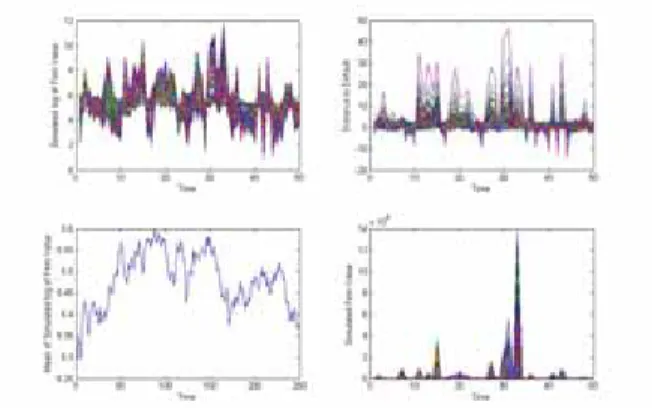
Simulation Results

In this article, there is no outlier in the simulation process and the auxiliary variable is not carried out. 50 particles are adopted in the simulated process, that is, there are 50 simulating paths in each experiment and each path contains 250 steps excluding the initial value. Monte Carlo simulation of the firm’s value and the distance to default is shown in figure 1.

The distance to default could not be evaluated directly. There are numerous variations in distance to default. The second procedure is to weight the sampling. The data with more information would be given more weights. There are about half of the density with lower weights. Thus, we take the higher weighted data to the next procedure. The Bayesian estimates of the weight are shown in the figure 2. The particles are not unevenly distributed and the weights are not quite equal. The filter approach could be applied in the next procedures.

After weighting the data with information content, the noises of the measurement process and the transition process could be calculated. The advanced estimate of the

distance to default is relatively stable. The main reason is the reduction of the noise contamination. As could be seen from the simulation results, particle filter is useful in eliminating the market noise in pricing the credit risk.

Fig. 1: Simulation of Firm’s Value and DD.

Fig. 2: The Bayesian Weights.

Fig. 3: Firm’s Market Value and DD with Particle Filter.

Traditional evaluation of firm’s market value in credit risk analysis could be easily contaminated by market noises. Those interruptions are irrational expectations. As could be referred from the result, the firm’s market value is hard to be evaluated

directly. With the adoption of particle filter approach, the pure market firm value could be calculated via the density of weighted re-samples with information content. The noises are also filtered out in the evaluation process. The remained data could be seen as the ones with fewer market noises. The estimated firm’s value could be seen as a real market value and the relative distance of default pricing of individual firm could be correctly calculated.

5.

Conclusion

In this study, the credit risk in distance to default is evaluated with particle filter approach. Due to the chaos in financial market, the evaluation of firm’s market value could be contaminated by the market noises. Particle filter could be adopted by Bootstrap alike weighted procedure in nonlinear and non-Gaussian formula to resolve the problem. The simulation results show that firm’s market value could be estimated purely and the relative variance is also evaluated with less noisy inflation. Thus, the distance to default with particle filter could be relatively properly evaluated.

References

Arulapalam, M. S., S. Maskell, N. Gordon, and T. Clapp, ‘‘A Tutorial on Particle Filters for Online Nonlinear/Non-Gaussion Bayesian Tracking,’’ IEEE Transactions on Signal Processing, Vol. 50, No. 2, pp. 174-188, 2002.

Black, F., and M. Scholes, ‘‘The Pricing of Options and Corporate Liabilities,’’ Journal of Political Economy, Vol. 81, No. 3, pp. 637-654, 1973.

Boyle, P. P., ‘‘Options: A Monte Carlo Approach,’’ Journal of Financial Economics, Vol. 4, pp. 323-338, 1977.

Bulter, A. W., and L. Fauver, ‘‘Legal and Economic Determinants of Sovereign Credit Ratings,’’ Working Paper, 2005.

Collin-Dufresne, P., R. S. Goldstein, and J. S. Martin, ‘‘The Determinants of Credit Spread Changes,’’ Journal of Finance, Vol. 56, No. 6, pp. 2177-2207, 2001. Doucet, A., S. Godsill, and C. Andrieu, “On Sequential Monte Carlo Sampling

Methods for Bayesian Filtering,” Statistics and Computing, Vol. 10, No. 3, pp. 197-208, 2000.

Duan, J. C., and A. Fulop, ‘‘Estimating the Structural Credit Risk Model When Equity Prices are Contaminated by Trading Noises,’’ Working Paper, 2005.

Elton, E. J., M. J. Gruber, D. Agrawal, and C. Mann, ‘‘Explaining the Rate Spread on Corporate Bonds,’’ Journal of Finance, Vol. 56, No. 1, pp. 247-277, 2001.

Gordon, N. J., D. J. Salmond, and A. F. M. Smith, ‘‘Novel Approach to Nonlinear/Non-Gaussian Bayesian State Estimation,’’ IEE Proceedings-F, Vol. 40, No. 2, pp.107-113, 1993.

Kisgen, D. J., ‘‘Credit Ratings and Capital Structure,’’ Journal of Finance, forthcoming.

Lin, M. T., J. L. Xhang, Q. Cheng, and R. Chen, ‘‘Independent Particle Filters,’’ Journal of the American Statistical Association, Vol. 100, No. 472, pp.1412-1421, 2005.

Merton, R. C., “On the Pricing of Corporate Debt: The Risk Structure of Interest Rates,” Journal of Finance, Vol. 29, No. 2, pp. 449-470, 1974.

Pitt, M. K., and N. Shephard, ‘‘Filter via Simulation: Auxiliary Particle Filters,’’ Journal of the American Statistical Association, Vol. 94, No. 446, pp. 590-599, 1999.

Vassalou, M., and Y. Xing, ‘‘Default Risk in Equity Returns,’’ Journal of Finance, Vol. 59, No. 2, pp.831-868, 2004.

Yu, F., ‘‘Accounting Transparency and the Term Structure of Credit Spreads,’’ Journal of Financial Economics, Vol. 75, No. 1, pp. 53-84, 2005.