國立臺灣大學理學院大氣科學所 碩士論文
Graduate Institute of Atmospheric Sciences College of Science
National Taiwan University Master Thesis
伴隨聖嬰現象西北太平洋反氣旋演變的研究 An Observational Study of Anomalous Anticyclone in
Western North Pacific Associated with El Niño
吳爾東 Erh-Tung Wu
指導教授:隋中興 教授
Advisor: Professor Chung-Hsiung Sui
中華民國 107 年 7 月
July 2018
摘要
聖嬰現象的強度隨著時間逐漸接近北半球冬季而達到高峰,此時由聖嬰現象 引發的環流異常和西北太平洋冬季季風交互作用通過 wind-evaporation-SST 回饋機 制(WES feedback)產生西北太平洋異常反氣旋(WNP AAC)(Wang et al. 2000),而這 個反氣旋距平並沒有隨著聖嬰事件消散並維持到聖嬰消退年的夏季 JJA(1)。為了 解釋聖嬰事件後西北太平洋異常反氣旋的維持機制,Xie et al.2009 提出 Indian Ocean Capacitor 機制,認為此時是由印度洋暖海溫加熱大氣在赤道西太平洋產生 Kelvin wave,進而導致西北太平洋低層輻散來維持西北太平洋反氣旋。Chung et al.
2011 則從西北太平洋副熱帶高壓的年際變化中分離出兩種時間尺度的振盪,週期 2-3 年的和反聖嬰現象有關,海洋大陸上的對流異常引發的局地哈德里環流在西北 太平洋產生下沉運動;週期 3-5 年的振盪則是由聖嬰現象透過 WES feedback 造成。
考慮到聖嬰事件之間消退速度的差異會對熱帶海表溫度、對流活動的分布產 生影響,本文將 1958-2016 年間的聖嬰事件依據聖嬰消退年夏季 JJA (1) Niño3.4 (170°-120°W, 5°S-5ׄ°N)海表溫度距平的三個月滑動平均即 Oceanic Niño Index (ONI) 作為指標,將聖嬰事件分為三類:fast-decay, slow-decay 以及 prolonged type。並利
用合成圖分析大尺度環流和海表溫度、視熱源(Q1)之間的關係,討論維持聖嬰事件
後夏季西太平洋反氣旋的機制是否會隨聖嬰事件相位有所不同。
當 ONI 在 JJA(1)下降到負值,意即聖嬰事件已經轉變至反聖嬰相位,稱為 fast- decay 事件;如果 ONI 仍然維持正值,則為 slow-decay 事件。如果到了下一個冬天 D(1)JF(2)還是維持聖嬰相位,就定義為 prolonged 事件。
在 fast-decay 事件中,WES feedback 從 D(0)JF(1)維持到 MAM(1),隨著反氣 旋南側的東風移入西太平洋,造成聖嬰事件在 JJA(1)快速轉變成反聖嬰相位。在反 聖嬰事件發生時,海洋大陸上異常旺盛的對流活動在西北太平洋產生對應的沉降 區,維持了西北太平洋反氣旋。Slow-decay 事件發展時類似 fast-decay 事件,但是 中太平洋上的暖海溫與異常對流持續到了夏天,所以 WES feedback 能夠維持作用。
而相對於前述兩類聖嬰事件,Prolonged 事件發展較慢,到了 MAM(1)才有明顯的 西北太平洋反氣旋,除了透過 WES feedback 在西北太平洋產生反氣旋環流之外,
海洋大陸上對流減弱引發的 Gill-Matsuno response 使得異常反氣旋延伸孟加拉灣。
從合成分析的結果來看,聖嬰現象的相位決定了 JJA(1)西北太平洋異常高壓
的維持機制。當 Niño3.4 SST 仍然是暖海溫異常時,WES feedback 就可以持續作 用。如果已經轉變成反聖嬰相位,西北太平洋反氣旋則是透過局地哈德里環流維持。
印度洋的角色在 fast-decay 事件中較為清楚,主要是幫助聖嬰現象的相位轉換(Kug and Kang 2006),到夏天印度洋海溫距平則已經消散。Prolonged 事件雖然在夏季伴 隨印度洋暖海溫異常,但是印度洋上卻是反氣旋環流,顯示此時海溫距平並沒有達 到加熱大氣的作用。唯在 Slow-decay 事件中,印度洋暖海溫距平有加熱大氣並引 發西太平洋東風異常提供西北太平洋負渦度,來維持反氣旋異常。
關鍵詞:年際變化、聖嬰現象、西北太平洋反氣旋、wind-evaporation-SST 回饋機 制、局地哈德里環流
Abstract
This is an observational analysis aimed to classify mechanisms for maintaining anomalous anticyclone (AAC) in western North Pacific (WNP) associated with El Niño events, especially in the El Niño decaying summer JJA(1) following the peak phase in winter D(0)JF(1). El Niño events from 1958-2016 are categorized into fast-decay, slow- decay, and prolonged types based on their Oceanic Niño Indices (ONI) in JJA(1) that are negative, positive, positive and followed by another El Niño event in the following winter, D(1)JF(2), respectively. Composite analysis is applied to anomalous fields of Sea Surface Temperature (SST), 850hPa stream function and vertically integrated apparent heat source 〈Q1〉 of the three types of El Niño events.
In the composite fields of the fast-decay type, the development of warm SST Anomaly (SSTA)/heating over equatorial Pacific is associated with an evolution of SSTA over Indian Ocean (IO) from a dipole pattern in SON(0) to basin wide warming in D(0)JF(1) and MAM(1). The heating associated with the IO SST evolution causes an eastward propagation of equatorial easterly anomalies (equatorial part of AAC) from eastern IO in SON(0)/ D(0)JF(1) to western Pacific in MAM(1) that results in a rapid phase transition into La Niña condition in JJA(1). The most evident maintenance mechanism for the WNP AAC is the wind-evaporation-SST (WES) feedback in D(0)JF(1) and MAM(1), and the strong La Niña heating contrast in JJA(1). The IO capacitor is only evident in MAM(1). The La Niña SST distribution and associated heating over the Maritime Continent in JJA(1) drives an overturning circulation with subsidence over WNP.
The composite fields of the slow-decay type and the prolonged type of El Niño events are generally similar except that the WNP AAC associated with the prolonged type emerges late in MAM(1). The WES feedbacks is the most evident mechanism
maintaining WNP AAC in D(0)JF(1) and MAM(1), and IO capacitor is evident in MAM(1) for the slow-decay type but not for the prolonged type. For both types of events, the AAC persists in JJA(1) with a broad zonal extent in the tropics (10°-30°N) from the dateline to the Bay of Bengal. Associated with the AAC for the slow-decay type, a zonal band of anomalous heating (cooling) exists between equator and 10°N (10°-20° N), and warm SSTA and anomalous heating also exist over northern IO. For the prolonged type, the heating over IO and western Pacific is weaker and more localized. The AAC in JJA(1) for the two types of El Niño is similar to the AAC found in Wang et al. (2013), Kosaka et al. (2013) and Li et al. (2017). The AAC appears to be maintained by a broader scale air- sea interaction involving extra tropical influence.
Keywords: interannual variability, El Niño, western North Pacific anomalous anticyclone, wind-evaporation-SST feedback, local Hadley circulation
Contents
Abstract (Chinese) --- i
Abstract (English) --- iii
Contents --- v
Table Captions --- vi
Figure Captions --- vii
Chapter 1 Introduction --- 1
Chapter 2 Data and Classification of El Niño --- 4
2.1 Data --- 4
2.2 Classification of El Niño --- 6
Chapter 3 Results --- 7
3.1 Fast-decay El Niño Events --- 7
3.2 Slow-decay El Niño Events --- 9
3.3 Prolonged El Niño Events --- 10
Chapter 4 Discussions and Empirical Orthogonal Function (EOF) Analysis --- 11
4.1 Discussions --- 11
4.2 Empirical Orthogonal Function (EOF) Analysis --- 13
Chapter 5 Conclusions --- 14
Reference --- 16
Appendix --- 19
Comparison of the Data Sets --- 19
Tables --- 22
Figures --- 23
Table Captions
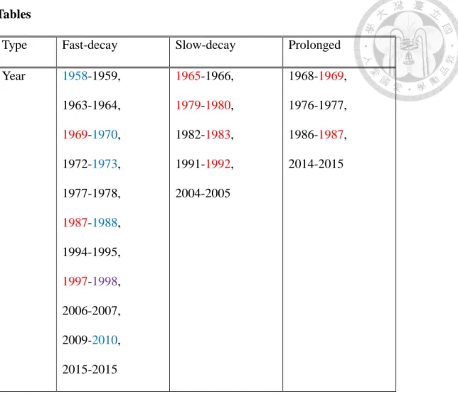
Table 1: The list of each El Niño type. The years with the principle component of the first EOF mode larger than one standard deviation are denoted in red, blue for the second mode, and purple for both.
Table 2: The list of years that the principle components are larger than one standard deviation (positive only) for the first two modes.
Figure Captions
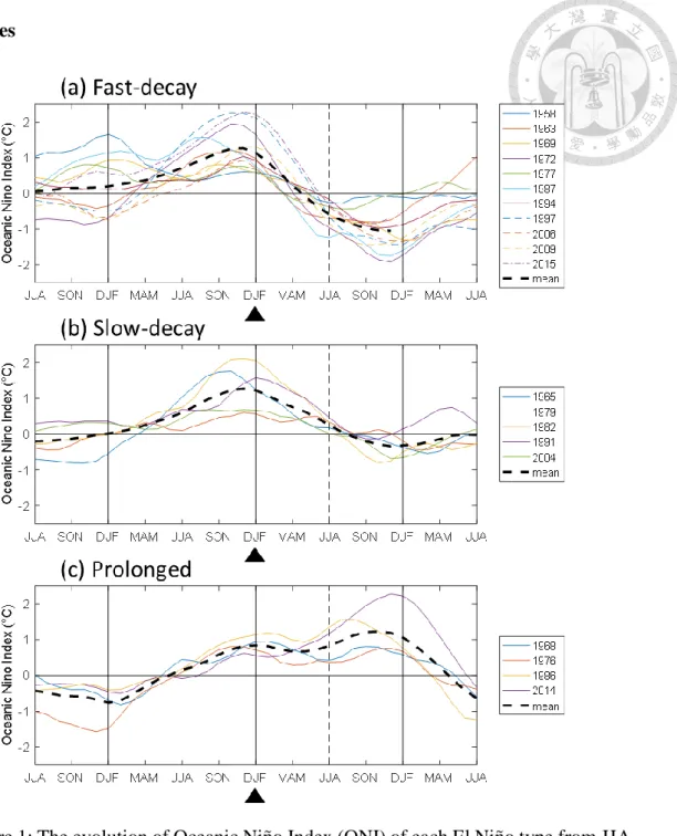
Figure 1: The evolution of Oceanic Niño Index (ONI) of each El Niño type from JJA (- 1) to JJA (2). Figure (a) for the fast-decay type, figure (b) for the slow-decay type, and figure(c) for the prolonged type El Niño. Black triangles indicate D(0)JF(1), and dashed lines indicate JJA(1) of each El Niño event. The line of the mean value of the fast-decay type ends at D(1)JF(2) because the datasets used in this study are from 1958JAN to 2016DEC. Thus, there is no data for year(2) of 2015-2016 event.
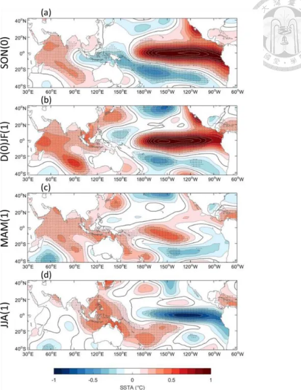
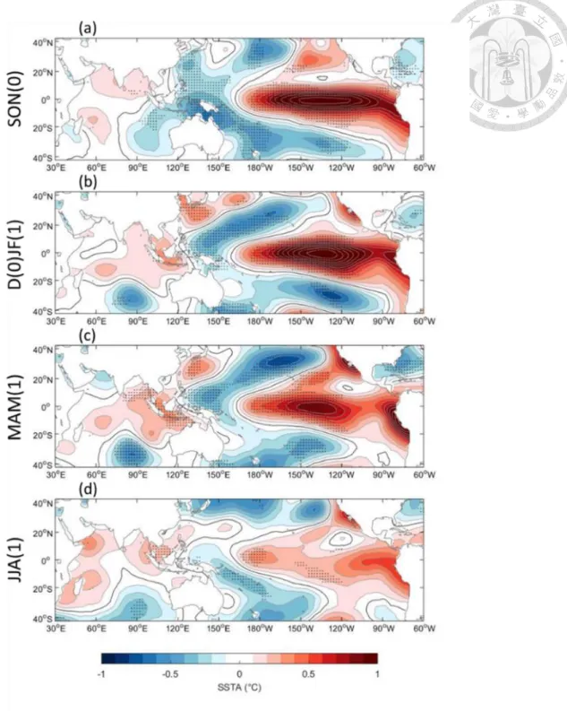
Figure 2: Composite maps for the fast-decay type El Niño events from SON(0) to JJA(1).
Shadings show SST anomalies (c.i. =0.2°C) and dotted area is for p-value<0.05.
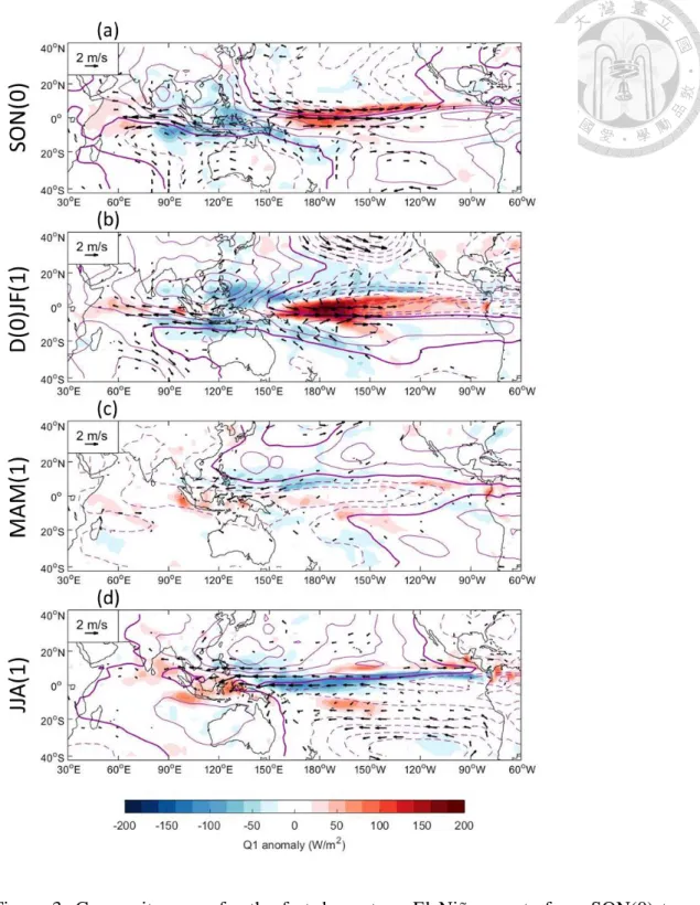
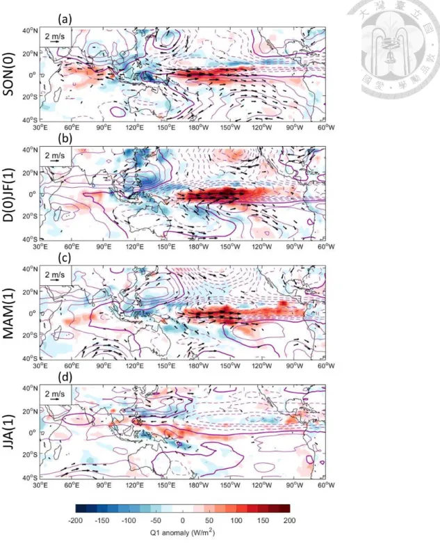
Figure 3: Composite maps for the fast-decay type El Niño events from SON(0) to JJA(1).
Shadings for 〈Q1〉 anomalies (c.i. =20 W/m2), vectors for 850hPa wind anomalies (p- value<0.15) and contours for 850hPa stream function anomalies (c.i = 100x106 m2/s; solid lines for positive values, dashed lines for negative values and thick solid lines for zero value).
Figure 4: Same as figure 2 but for the slow-decay type.
Figure 5: Same as figure 3 but for the slow-decay type.
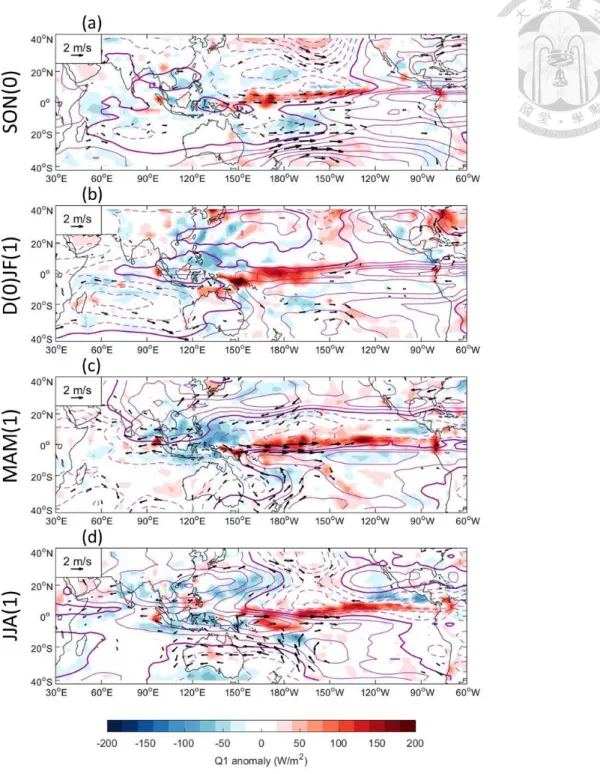
Figure 6: Same as figure 2 but for the prolonged type.
Figure 7: Same as figure 3 but for the prolonged type.
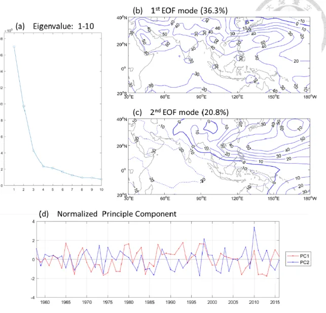
Figure 8: Empirical orthogonal functions (EOF) analysis of JJA 850hPa geopotential height over Asian-Australian monsoon domain (20°S-40°N, 30°-180°E). Figure (a) is the eigenvalue for the largest 10 modes. The contour of figure (b) is the pattern of the 1st EOF mode, and the figure(c) for the 2nd EOF mode. Figure (d) is the normalized principle component of the 1st and the 2nd EOF mode.
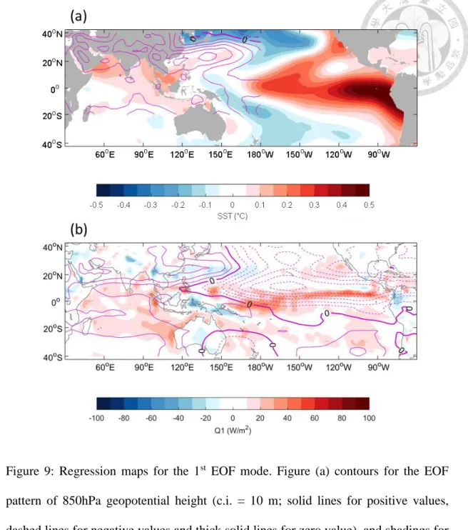
Figure 9: Regression maps for the 1st EOF mode. Figure (a) contours for the EOF pattern of 850hPa geopotential height (c.i. = 10 m; solid lines for positive values, dashed lines
for negative values and thick solid lines for zero value), and shadings for the regression of SST on normalized principle component of the 1st EOF mode. Figure (b) contours for the regression of 850hPa stream function (c.i. = 50x106 m2/s; solid lines for positive values, dashed lines for negative values and thick solid lines for zero value), and shadings for the regression of 〈Q1〉 on normalized principle component of the 1st EOF mode.
Figure 10: Same as figure 13 but for the 2nd EOF mode.
Figure 11: The comparison of 850hPa geopotential height from ERA-40 and ERA- interim for each season during the overlapping period (January 1979 to August 2002).
Shadings present root-mean-square of the difference between 850hPa geopotential height from ERA-40 and ERA-interim (c.i. = 1 m). Contours shows the seasonal mean of 850hPa geopotential height from ERA-interim (c.i. = 50 m). The gray shadings indicate the areas with a topography higher than 1500 m.
Figure 12: Same as figure 1 but for 850hPa U-wind component (c.i. = 0.2 for shadings;
c.i. = 4 m/s for contours).
Figure 13: Figure 13: Same as figure 1 but for 850hPa V-wind component (c.i. = 0.2 for shadings; c.i. = 2 m/s for contours).
Figure 14: The Hovmöller diagram for the difference of 850hPa geopotential height between ERA-40 and ERA-interim. Shadings show the evolution of the meridional averaged difference (ERA-interim minus ERA-40, c.i. = 1m) between these two datasets.
Contours indicate the 3-month running averaged value of meridional averaged 850hPa geopotential height from ERA-interim (c.i. = 50 m). Figure (a) for 15°S-25°S, figure (b) for 5°S-5°N, and figure (c) for 15°N-25°N.
Figure 15: Same as figure 14 but for 850hPa U-wind component (c.i. = 0.2 for shadings;
c.i. = 4 m/s for contours).
Figure 16: Same as figure 14 but for 850hPa V-wind component (c.i. = 0.2 for shadings;
c.i. = 2 m/s for contours).
Figure 17: Seasonal composite maps for the vertically integrated apparent heat source (〈Q1〉) and GPCP precipitation rate. Shadings for 〈Q1〉 (c.i. = 50 W/m2) and contours for the precipitation rate (c.i. = 50 W/m2, 1 mm/day ~ 29 W/m2).
Figure 18: Seasonal composite maps for the radiation heating (〈QR〉) (c.i. = 50 W/m2).
Figure 19: Seasonal composite maps for the net condensation heating (LP) derived from
〈Q1〉 and GPCP precipitation rate. Shadings for LP (c.i. = 50 W/m2) and contours for the precipitation rate (c.i. = 50 W/m2).
Figure 20: Shading shows the correlation coefficient between precipitation data from GPCP and the heating rate of net condensation derived from 〈Q1〉 for each season.
Contours indicate the annual mean precipitation rate from GPCP (c.i. = 50 W/m2).
Figure 21: Seasonal composite maps for the vertically integrated apparent moisture sink (〈Q2〉) and GPCP precipitation rate. Shadings for 〈Q2〉 (c.i. = 50 W/m2) and contours for the precipitation rate (c.i. = 50 W/m2).
Figure 22: Seasonal composite maps for the surface latent heat flux (-LE) (c.i. = 50 W/m2).
Figure 23: Seasonal composite maps for the net condensation heating (LP) derived from
〈Q2〉 and GPCP precipitation rate. Shadings for LP (c.i. = 50 W/m2) and contours for the precipitation rate (c.i. = 50 W/m2).
Figure 24: Shading shows the correlation coefficient between precipitation data from GPCP and the heating rate of net condensation derived from 〈Q2〉 for each season.
Contours indicate the annual mean precipitation rate from GPCP (c.i. = 50 W/m2).
Chapter 1 Introduction
The influence of El Niño and Southern Oscillation (ENSO) on global climate has been studied extensively since the Tropical Ocean – Global Atmosphere (TOGA) era (e.g.
Trenberth et al. 1998; Alexander et al. 2002). About the regional influence of warm ENSO on East Asian monsoon variation, a particular important feature is the low-level anomalous anticyclone (AAC) over the western North Pacific (WNP) that develops from the ENSO developing fall (SON(0)) through the following spring (MAM(1)) /summer (JJA(1)).(e.g. Tanaka 1997) (The seasons are referred to Northern Hemisphere in this article.) The prolonged existence of the AAC is attributed to a Rossby wave response to cold sea surface temperature anomaly (SSTA) that is maintained by local air-sea heat exchanges (Wang 2000, 2002). The Matsuno-Gill response of the enhanced convection activity over Central Pacific causes anomalous northeasterly winds on WNP, and cools the local SST through Wind-Evaporation-SST (WES) feedback by strengthening the winter monsoon. The cold SSTA over WNP stabilizes lower atmosphere, suppresses convection, and induces atmospheric anticyclonic flow in the northwest via Rossby Wave response. As the anomalous northeasterly in the southeast quadrant of the AAC enhances the trade wind speed, the evaporation rate increases and feeds back to cold SSTA.
The above air-sea coupling requires the existence of equatorial heating and background northeasterly monsoon flow to enhance evaporation and cooling SSTA. It is criticized that this required condition is absent in the decaying summer when monsoon flow reverses and the trade winds retreat eastward away from the WNP, so the cold SSTA often weakens and vanishes (Xie et al. 2009). On the other hand, Wang et al. (2013) showed that even in JJA, mean northeasterly still existed in subtropical WNP, and supported the WES feedback between cold SST and AAC. Taking into account of the persistent Indian Ocean (IO) warming following the El Niño development till summer,
some studies proposed that the IO warming in El Niño peaking DJF acted like a discharging capacitor to maintain the WNP AAC in the following summer (Yang et al.
2007, Xie et al. 2009, 2016). The anomalous Walker circulation excites oceanic downwelling Rossby wave in the southeastern IO during the peak winter of El Niño, causing SST warming over the southwestern IO in the following spring and summer. The IO SSTA pattern induces a basin-wide SST warming in next summer via decreasing Indian monsoon wind speed. The easterlies associated with the atmospheric Kelvin wave response to the IO SST warming then maintain the AAC over WNP in JJA (1).
In addition to the IO warming, Terao and Kubota (2005) indicated that the interbasin SST anomaly contrast between warm IO and cold WNP was also an important feature that maintained the WNP AAC in the post El Niño summer. The easterlies of Kelvin wave response to the SSTA contrast result in off-equatorial low-level divergence, which forms the eastern part of the AAC. The suppressed rainfall over the low-level divergence further emanates anticyclonic Rossby waves and the AAC is thus extended westward. Yun et al.
(2013) addressed respective delayed impacts of SSTA from IO warming, West Pacific cooling and East Pacific cooling. They showed that the enhanced WNP subtropical high was a result of combined effect of IO warming and WP cooling, and that concurrent EP cooling could strengthen North Pacific high.
In view of the interannual oscillations of WNP AAC, Chung et al. (2011) found that the WNP AAC followed ENSO evolution at two distinct time scales, 2-3 year and 3-5 year. The AAC in 2–3 year oscillation exhibits an eastward propagating feature in corresponding SST anomaly, residing in the sinking branch of the local Hadley circulation due to enhanced convection over the Maritime Continent. The AAC possesses a barotropic vertical structure and is maintained by radiative cooling. The AAC in 3–5 year oscillation shows a quasi-stationary feature with enhanced convection over Central
Pacific (CP) and central IO. The maximum sinking motion is located southeastern to the WNP AAC center. The AAC acquires a baroclinic vertical structure. The overall features suggest the AAC with a 3-5 year period is a Rossby wave response to a persistent local cold SSTA associated with negative latent heat fluxes.
From the perspective of predictability of East Asia Monsoon, both Wang et al. (2013) and Kosaka et al. (2013) proposed that WNP AAC was a part of atmosphere-ocean coupled system over Indo-Pacific warm pool. Identifying from the first EOF mode of JJA 850hPa geopotential height over the Asian-Australian monsoon area, Wang et al. (2013) attributed the WNP AAC to broad SSTA contrast between warm northern IO and cold WNP, and the WNP AAC reinforced SSTA gradient by latent heat flux exchange anomalies related to strengthened WNP northeasterlies and relaxed IO southwesterlies.
The second EOF mode identified in Wang et al. (2013) is linked to a La Niña-like SSTA pattern and enhanced precipitation over the Maritime Continent, which is similar with the 2-3 year oscillating AAC reported by Chung et al. (2011). Kosaka et al. (2013) interpreted that the Kelvin Waves excited from warm northern Indian Ocean into WNP induced off- equatorial divergence and maintained the WNP AAC, whose westward extension into northern IO is, as suggested by Terao and Kubota (2005), a downwelling Rossby response to the suppressed WNP convection. They reasoned that northern IO is warmed by enhanced insolation due to clear sky under AAC and relaxation of mean southwesterlies by anomalous easterlies in the southern flank of AAC. Both studies (Wang et al., 2013;
Kosaka et al., 2013) conducted atmosphere-ocean coupled experiments to confirm the concept of the large-scale unstable coupled system, which could exist without but strongly excited by ENSO.
In a review article, Li et al. (2017) suggested that the above studies of interbasin atmosphere–ocean interaction across the Indo-Pacific warm pool is a new mechanism for
maintaining the summertime AAC over the western North Pacific. In addition, Li et al (2017) also added the moist enthalpy advection/Rossby wave modulation to the WES feedback mechanism as essential for the initial development and maintenance of the WNP AAC during El Niño mature winter and subsequent spring. As discussed above, the maintenance of WNP AAC through El Niño decaying seasons is complexed with several mechanisms and involves SST distributions in both Pacific and Indian Ocean. Hence, in order to clarify the roles of each process in observation, it is straightforward to investigate the maintenance of WNP AAC with respect to classified conditions of ENSO in decaying JJA. However, to the best of knowledge, only Yun et al. (2013) did separate different ENSO events, yet their classification accorded to the SSTA in El Niño peaking DJF instead of the subsequent JJA, during which signals could be mixed up potentially. The objective of this study is to analyze the evolution of SST distribution and associated climate anomalies for different types of El Niños that show fast decay, slow decay, or persistence in Niño3.4 SSTA during post-El Niño summer.
Chapter 2 Data and Classification of ENSO 2.1 Data
The data set used in this study covers a 59-year time span from 1958 to 2016. We adopt reanalysis data from the European Centre for Medium-Range Weather Forecasts (ECMWF) including wind, p-velocity, geopotential height, temperature and specific humidity fields for each pressure level and mean sea-level pressure for the surface level.
In order to analyze as many events as possible, the dataset is combined from monthly data of ECMWF ERA-40 (Uppala et al. 2005) and ERA-Interim (Dee et al. 2011). The temporal span is September 1957 to August 2002 for ERA-40, and January 1979 to present for Interim. First, the horizontal grid size of ERA-Interim is linearly interpolated
from 1.5° by 1.5° to 2.5° by 2.5° to be consistent with that of ERA-40. In the overlapping period (January 1979 to August 2002) of two datasets, values of two datasets are averaged to obtain a combined dataset of longer time span. The two data sets are compared as discussed in the appendix.
The abnormal large-scale circulation induced by El Niño is represented by 850hPa stream function (ψ) anomaly. The monthly data of 850hPa stream function is derived from the monthly data of 850hPa horizontal wind and density according to the following equations.
𝑉⃑ = 𝑉⃑ 𝑟𝑜𝑡+ 𝑉⃑ 𝑑𝑖𝑣, (1) 𝑉⃑ 𝑟𝑜𝑡 = 𝑘̂ × ∇𝜓, (2) 𝑉⃑ 𝑑𝑖𝑣 = ∇𝜒, (3) Where 𝑉⃑ 𝑟𝑜𝑡 is the rotational wind, 𝑉⃑ 𝑑𝑖𝑣 is the divergence wind, 𝜌 is the density of air, 𝜓 is the stream function, and 𝜒 is the velocity potential. Because the large-scale circulation is quasi-geostrophic, we choose 850hPa stream function to represent the anomalous anticyclone in western north Pacific.
To represent the large-scale atmospheric heating before satellite era, vertically integrated heat source (〈Q1〉) and moisture sink (〈Q2〉) are both calculated from 6-hourly data of ERA-40 and ERA-interim from surface to 100hPa according to the following equations.
s = 𝐶𝑝𝑇 + 𝑔𝑧 (4)
h = 𝐶𝑝𝑇 + 𝑔𝑧 + 𝐿𝑞 (5)
〈𝑄1〉 =1
𝑔∫𝑃𝑃𝑠𝑓𝑐𝑄1𝑑𝑝
𝑡𝑜𝑝 = 1
𝑔∫ (𝜕𝑠
𝜕𝑡+ ∇ ∙ 𝑠𝑉 +𝜕𝑠𝜔
𝜕𝑝) 𝑑𝑝
𝑃𝑠𝑓𝑐
𝑃𝑡𝑜𝑝 (6)
〈𝑄2〉 = 1
𝑔∫𝑃𝑃𝑠𝑓𝑐𝑄2𝑑𝑝
𝑡𝑜𝑝 = −𝐿
𝑔∫ (𝜕𝑞
𝜕𝑡+ ∇ ∙ 𝑞𝑉 +𝜕𝑞𝜔
𝜕𝑝) 𝑑𝑝
𝑃𝑠𝑓𝑐
𝑃𝑡𝑜𝑝 (7)
Where
〈 〉 =1
𝑔∫𝑃𝑃𝑠𝑓𝑐( )𝑑𝑝
𝑡𝑜𝑝 (8) The sea surface temperature data is from National Oceanic and Atmospheric Administration (NOAA)’s Extended Reconstructed Sea Surface Temperature (ERSST) version 4 (Huang et al. 2015).
Anomaly values are calculated as the deviation from monthly means of 1958-2016 climatology. The linear trend is removed from anomalies, and then three-month running mean is applied.
2.2 Classification of El Niño
The Oceanic Niño Index (ONI) from NOAA’s Climate Prediction Center is considered to represent El Niño evolution. ONI is defined as 3-month running-mean SSTA over Niño3.4 region (170°-120°W, 5°S-5°N).
The warm phase of ENSO, or the periods of El Niño from 1958-2016 are identified based on ONI following NOAA´s definition that periods with ONI above 0.5°C for at least of 5 consecutive months. Each boreal winter in the El Niño period is counted as an El Niño event since an El Niño always peaks at DJF. Observed El Niño events are categorized into fast-decay, slow-decay, and prolonged types, based on its ONI in the decaying summer, June-July-August, JJA(1). The El Niño events that decay quickly and have negative ONI in JJA(1) are defined as the fast-decay type events, and those events that have positive ONI in JJA(1) are the slow-decay type events. Furthermore, if ONI remains above 0.5 in the following winter, or D(1)JF(2), the event is defined as a prolonged El Niño. The only excluded event is 2002/03, because its ONI dropped below zero in the decaying April-March-June, but turned positive in JJA(1) again. The result of the classification is shown in Table 1. There are 11 fast-decay events, 5 slow-decay events
and 4 prolonged events. The ONI evolution of each El Niño type from JJA(-1) to JJA(2) is presented in figure 1.
Chapter 3 Results
The following results are based on the composite analysis of SSTA, low-level circulation and vertically integrated apparent heat source (〈Q1〉) anomalies of each El Niño type from the developing boreal falls to the following summers. All three types of El Niño events have an anomalous anticyclone over western North Pacific (WNP AAC) in JJA(1), but only fast and slow-decay types have WNP AAC during the El Niño mature winters, and the WNP AAC in the prolonged type establishes in the following springs.
3.1 Fast-decay El Niño Events
Figure 2 and figure 3 show the composite of SST anomaly, 850hPa stream function anomaly and 〈Q1〉 anomaly of the fast-decay El Niño evolution from developing falls, SON(0) to following summers, JJA(1). The fast-decay El Niño is accompanied by a positive Indian Ocean Dipole (IOD) of fair magnitude in SON(0), so the SSTA field is featured with three poles at the equator, which are heating, cooling, heating over CP, Eastern IO, Western IO, respectively. These SSTA poles drive corresponding 〈Q1〉 anomalies showed in figure 3, establish anomalous Walker Circulation, and induce a strong low-level quadrupled circulation by Gill-Matsuno type response; the quadruple symmetrical about the equator is composed of a pair of cyclones east and anticyclones west to the cooling center. The AAC is located over North IO, in the northwestern quadrant of the quadruple. It is the South IO AAC that drives oceanic downwelling Rossby Waves which deepen the thermocline and warm SST of the southwestern IO in the following seasons, as the charging stage of the IO capacitor effect.
In El Niño peaking winter (D(0)JF(1)), IOD mode change into a basin-wide warm SSTA, Indian Ocean Basin (IOB) mode while the SSTA pattern over the tropical Pacific remains El Niño condition and the quadruple circulation continues to dominates the low- level atmosphere, with its western components slightly shifting eastward. This shift is triggered by the abrupt demise of the eastern pole of IOD, and further amplified by WES feedback given by the background northeasterly. This coupling is supported by the synchronous migration of the maximum cold SSTA and atmospheric cooling from Eastern IO to WP.
In the following spring (MAM(1)), the local WES feedback may still exists over WNP remains clear, as indicated by the cold SSTA and anomalous northeasterly. Because the EP SSTA decays dramatically, the anomalously reversed Walker Circulation weakens and the suppressed convection as well as accompanying anomalous low-level divergence around WP/Maritime Continent diminishes. Since the westerly eastern to the divergence disappears, the equatorial easterly over WP, induced by Kelvin Wave response to the atmospheric heating and warm SSTA over tropical IO, is no longer counteracted, and supports the AAC vorticity. This easterly may also feedback to El Niño decay via triggering oceanic upwelling Kelvin Waves.
In JJA(1), the SSTA over Tropical Pacific turns to a La Niña condition, and the 〈Q1〉 anomaly shows strong atmospheric heating over eastern IO and Maritime Continent, and cooling over tropical Pacific and WNP. The strong enhanced convection is located around Maritime Continent and contributes to the sinking motion of WNP AAC in form of local Hadley Circulation. On the other hand, the equatorial easterly forced by zonal SSTA gradient of La Niña can also support WNP AAC by providing negative vorticity.
3.2 Slow-decay El Niño Events
Figure 4 and figure 5 show the composite of slow-decay type. For the slow-decay events, the composite fields of SSTA, circulation and 〈Q1〉 are similar to those of the fast- decay events in El Niño developing fall (SON(0)) and winter (D(0)JF(1)), but with IO feature of weaker amplitude. In SON(0), there is still a clear IOD pattern over IO but it does not turn into a strong IOB in D(0)JF(1), compared with the fast-decay type. Instead of forming a large anticyclone extended from IO to WNP like the fast-decay type, the eastward migration of the AAC from North IO to WNP in the El Niño peak winter with clear WES feedback over WNP in the slow-decay type events. In D(0)JF(1) of the slow- decay type, the cold SSTA over WNP is even stronger than the fast-decay type.
In MAM(1), because the EP SSTA remains fairly warm, the anomalously reversed Walker Circulation over the tropical Pacific is still strong, so the divergence over Maritime Continent contributes to part of the AAC over IO. The local cold SSTA southeast to the WNP AAC also continue to support it via WES feedback. Because there is still atmospheric cooling over the Maritime continent, the AAC does not shift eastward, like the one in the fast-decay type.
In JJA(1), the SSTA pattern is still a weak El Niño condition with warm SSTA over tropical CP, EP and IO but the cold core of SSTA over WP moves from WNP to southern hemisphere. The pattern of 〈Q1〉 anomaly shows a band of heating anomaly extends from northern IO to tropical central Pacific and cooing anomaly over WNP and New Guinea and forms a pattern similar to the Pacific-Japan pattern. Compared to WNP AAC in MAM(1), WNP AAC in JJA(1) shifts to the northern subtropics (10°-30°N). The AAC over WNP can still be maintained by the Rossby response to the SSTA west to the AAC itself while the contrast heating between northern IO and WNP induces easterly anomaly that can sustain the WNP AAC by low level divergence.
3.3 Prolonged El Niño Events
Figure 6 and 7 show the composite evolution of the prolonged type events from SON(0) to JJA(1). During the developing fall (SON(0)), the SSTA pattern over the tropical IO and the maritime continent is less prominent compared to the fast-decay and slow-decay cases, so the anticyclone pairs that appear in the fast-decay and slow-decay composites are unclear. The SSTA is significant over the southwestern IO, the central and eastern Pacific.
Because AAC does not form in IO in SON(0), there is no AAC shift from North IO to WNP in D(0)JF(1) in the prolonged type. As the result, the AAC in the northwestern quarter of the quadruple barely exists in D(0)JF(1) even though the prolonged events cause negative 〈Q1〉 anomaly over WNP by WES feedback in figure 6.b. On the other hand, convection activity is suppressed over western tropic IO, and an AAC is located over south IO.
In MAM(1), the suppressed convection organizes around Eastern IO and Maritime Continent. In response to the organized atmospheric cooling over Maritime Continent and atmospheric heating over central tropical Pacific, the anomalous circulation forms a quadrupole structure with a pair of anticyclones over IO and a pair of cyclones over central tropical Pacific. It is also noted that the AAC extends northeastward, and forms a secondary maximum over extratropical North Central Pacific in MAM(1). Because of the atmospheric cooling and northeasterly anomaly located at the southeastern of WNP AAC, it is convincing that the positive stream function anomaly over WNP is maintained by WES feedback. The positive SSTA over the IO basin does not trigger significant atmospheric heating so the warn IO should be the result of the increased solar radiation caused by suppressed convections.
In JJA(1), patterns of SSTA, 〈Q1〉 anomaly and 850hPa steam function anomaly do
not change much from the ones in MAM(1). The AAC over WNP still exists because the El Niño condition persists and induces atmospheric cooling over WNP by WES feedback.
Although the warm SSTA appears across IO basin, it does not conduct significant large- scale atmospheric heating. Thus, the IO SSTA is suggested to play a passive role.
Chapter 4 Discussions and Empirical Orthogonal Function Analysis 4.1 Discussions
Our results show that the WNP AAC does exist in all three types of El Niño events in the decaying summer categorized by this study (Figure 3d, 5d, and 7d). However, the evolution of the WNP AAC reveals different features in the three types of events.
WES feedback maintains the WNP AAC in the fast-decay (Figure 2b, 3b) and slow- decay type (Figure 4b, 5b) events in the El Niño peak winter, and works in all three types in the following spring, MAM(1). In contrast to the other two types, the fast-decay type of events reveals a dramatic decay in SSTA over equatorial Pacific from MAM(1) to JJA(1), and convective heating over the Maritime Continent/eastern IO and cooling over equatorial Pacific in JJA(1) is the key forcing for the maintenance of WNP AAC.
During boreal summers, northeasterly trades still dominate background winds over subtropical WNP (Wang et al., 2013), while in the slow-decay and prolonged composite fields, atmospheric cooling and associated cold SSTA remain weak in the AAC’s southeast quadrant. It suggests that in slow-decay or prolonged events, WES feedback can partly maintain WNPAC in JJA(1). In addition, the warm SSTA over tropical CP in the slow-decay and prolonged events maintains the heating source that triggers northeasterly anomaly over subtropical CP.
In the fast-decay events, the SSTA over equatorial Pacific is in La Niña condition, and WNP AAC resides in the subsidence of a strengthened local Hadley circulation induced
by the enhanced convection over Maritime Continent and cooling to the east.
The result is consistent with Chung et al. 2011, which also pointed out that the enhanced convection over Maritime Continent is important for 2-3 years oscillation and the warm CP SSTA is respectively important in 3-5 years oscillation of summertime WNP AAC.
The role of IO SSTA also differs from type to type. In the fast-decay type, the strongest IO warming appears in D(0)JF(1) and gradually decays in the following seasons. In MAM(1), warm SSTA and heating over eastern IO excite easterly anomalies over WP with atmospheric Kelvin wave dynamics. The easterlies cool down central/eastern Pacific SSTA by inducing oceanic upwelling Kelvin wave, so the warm IO condition is essential for fast-decay events (Kug and Kang 2006). In JJA(1), warm SSTA over IO decays dramatically especially over western and central IO, and warm IOB does not exist.
In contrast, in the slow-decay type and the prolonged type, the warm SSTA over IO persists from D(0)JF(1) to JJA(1) because the El Niño condition stays longer. However, the IO SSTA has different roles in those two types.
During JJA(1), in the slow-decay type, the warm SSTA drives atmospheric heating over northern IO. The heating-cooling contrast between northern IO and WNP excites easterly anomalies over WNP and South China Sea. The easterlies provide negative vorticity on the poleward side. and also warms the SSTA over the Bay of Bengal and South China Sea by relaxation of monsoon westerlies. Thus, in slow-decay events, the WNPAC during JJA(1) is a part of the unstable atmosphere-ocean coupled mode (Wang et al., 2013; Kosaka et al., 2013).
Although during JJA(1), the warm SSTA over IO in the prolonged type is relatively strong, they collocates with scattered atmospheric cooling, which suggests that the warm IO SSTA play a passive role. Because the El Niño condition continues, WNP AAC is still
maintained by WES feedback associated with the cold SSTA and atmospheric cooling over its southeast flank, while its extension into the northern IO is the Gill-Matsuno response of the atmospheric cooling over Maritime Continent.
4.2 Empirical Orthogonal Function (EOF) Analysis
According to Wang et al. (2013), the interannual variance of the western Pacific subtropical high can be explained by the first two EOF modes of JJA 850hPa geopotential height over the Asian-Australian monsoon domain (30°-180°E, 20°S-40°N). The first mode is due to the thermodynamic feedback of surface flux response to WES feedback induced by the strengthened western Pacific Subtropical High, and the principle component is not well correlated with simultaneous Niño 3.4 SSTA. The second mode is linked with a developing or persisting La Niña event.
To compare with our results, we applied the same EOF analysis (Figure 8) but for a longer time period (1958-2016) than Wang et al. (2013) (1979-2009) by using the combined data of ERA-40 and ERA-interim and regressed SST, 850hPa stream function,
〈Q1〉 to the normalized principle component of the first mode (36.3%) and the second mode (20.8%). Figure 9 shows the regression maps of the first mode and resemble the composite maps of the slow-decay El Niño in the decaying summer (Figure 4d, 5d).
Figure 10 shows the regression maps of the second mode and resemble the composite maps of the fast-decay El Niño in the decaying summer (Figure 2d, 3d). Also, the list of the years for the principle components larger than one standard deviation is presented in Table 2. By comparing Table 2 and Table 1, we found that the pattern of the first EOF mode happens in the developing phase of El Niño or the decaying phase of the slow- decay and prolonged type events, and the second EOF mode appears in the decaying year of the fast-decay El Niño events.
Chapter 5 Conclusions
The mechanisms to maintain the summertime low-level anomalous anticyclone (AAC) over western North Pacific (WNP) are clarified, with respect to different El Niño conditions during the decaying summer, JJA(1). Observed El Niño events from 1958- 2016 are categorized into fast-decay, slow-decay, and prolonged types, based on ONI in JJA(1). Composite method is utilized to analyze the sea SSTA, low-level atmospheric circulation and rainfall.
The composite fields of the fast-decay events in El Niño developing fall, SON(0), are featured with a strong low-level quadrupled circulation, driven by tripole heating distribution (heating-cooling-heating) over tropical Eastern Pacific (EP)-Eastern Indian Ocean (IO)-Western IO that correspond to warm-cold-warm SSTA. The AAC is located over IO, in the northwestern quarter of the quadruple. In the following winter DJF(1), the cooling center and the AAC migrate eastward from Eastern IO to Western Pacific (WP) because of the abrupt demise of the Eastern IO pole and Wind-Evaporation-SST (WES) feedback. During MAM(1), the local WES feedback over WNP is still clear, but the EP SSTA decays so dramatically that the IO Capacitor Effect (IOCE) manifests significantly.
In JJA(1), the equatorial Pacific turns to a La Niña condition, and the AAC is largely maintained by equatorial atmospheric cooling associated with cold SSTA over EP.
For the slow-decay type, its SSTA and atmospheric circulation patterns are similar to the fast-decay type in the El Niño developing seasons. However, the El Niño condition remains so the WNP AAC is maintained by the WES feedback caused by the warm SSTA over tropical CP. On the other hand, SSTA contrast over WP and northern IO induces easterly anomaly that provides negative vorticity to WNP AAC.
The composite fields of prolonged events show a relatively weak AAC, equatorial Pacific SSTA, and IO SSTA during SON(0), compared with those of fast-decay events.
The AAC does not form clearly until MAM(1), which might be attributed to a band of uniform atmospheric cooling over southern tropical IO in SON(0) and D(0)JF(1). The AAC is then maintained by persistent equatorial Pacific warm SSTA from MAM(1) to SON(1); thus, it stays almost stationary over India and South Asia. Although IO does warm from MAM(1) to JJA(1), they are mainly corresponded to atmospheric cooling, which suggests that IO plays a passive role.
This study shows that WNP AAC in the following summers can be resulted from different mechanisms in different types of El Niño. In the fast-decay type, the AAC is in the subsidence area of the local Hadley cell induced by the enhanced convections over the maritime continent. In the slow-decay and the prolonged types, the AAC is anchored in WNP because the warm phase of ENSO still maintains the WES feedback.
Reference
Alexander, M.A., I. Bladé, M. Newman, J.R. Lanzante, N. Lau, and J.D. Scott, 2002: The Atmospheric Bridge: The Influence of ENSO Teleconnections on Air–Sea Interaction over the Global Oceans. J. Climate, 15, 2205–2231.
Chung, P. H., C.-H. Sui, and T. Li, 2011: Interannual relationships between the tropical sea surface temperature and summertime subtropical anticyclone over the western North Pacific. J. Geophys. Res.: Atmos., 116(13).
Dee, D. P., Uppala, S. M., Simmons, A. J., Berrisford, P., Poli, P., Kobayashi, S., Andrae, U., Balmaseda, M. A., Balsamo, G., Bauer, P., Bechtold, P., Beljaars, A. C. M., van de Berg, L., Bidlot, J., Bormann, N., Delsol, C., Dragani, R., Fuentes, M., Geer, A.
J., Haimberger, L., Healy, S. B., Hersbach, H., Hólm, E. V., Isaksen, L., Kållberg, P., Köhler, M., Matricardi, M., McNally, A. P., Monge-Sanz, B. M., Morcrette, J.-J., Park, B.-K., Peubey, C., de Rosnay, P., Tavolato, C., Thépaut, J.-N. and Vitart, F.
2011: The ERA-Interim reanalysis: configuration and performance of the data assimilation system. Q. J. R. Meteorol. Soc., 137: 553–597.
Huang, B., P. Thorne, T. Smith, W. Liu, J. Lawrimore, V. Banzon, H. Zhang, T. Peterson, and M. Menne, 2015: Further Exploring and Quantifying Uncertainties for Extended Reconstructed Sea Surface Temperature (ERSST) Version 4 (v4). J. Climate, 29, 3119–3142, doi:10.1175/JCLI-D-15-0430.1
Izumo, T., J. Vialard, H. Dayan, et al., 2016: Clim. Dyn. 46, 2247.
https://doi.org/10.1007/s00382-015-2700-4
Kosaka Y, S. P. Xie, N. C. Lau, and G. A. Vecchi, 2013: Origin of seasonal predictability for summer climate over the Northwestern Pacific. Proc. Natl. Acad. Sci. USA 110(19):7574–7579.
Kug, J. and I. Kang, 2006: Interactive Feedback between ENSO and the Indian Ocean. J.
Climate, 19, 1784–1801.
Li, T., B. Wang, B. Wu, et al., 2017: Theories on formation of an anomalous anticyclone in western North Pacific during El Niño: A review. J. Meteor. Res., 31(6), 987–1006, doi: 10.1007/s13351-017-7147-6.
Terao, T., and T. Kubota, 2005: East-west SST contrast over the tropical oceans and the post El Niño western North Pacific summer monsoon. Geophys. Res. Lett., 32(15) , L15706, doi: 10.1029/2005GL023010.
Trenberth, K. E., G. W. Branstator, D. Karoly, A. Kumar, N.-C. Lau, and C. Ropelewski, 1998: Progress during TOGA in understanding and modeling global teleconnections associated with tropical sea surface temperatures, J. Geophys. Res., 103(C7), 14291–
14324, doi:10.1029/97JC01444.
Uppala, S. M., and Coauthors, 2005: The ERA-40 Re-Analysis. Quart. J. Roy. Meteor.
Soc., 131, 2961–3012.
Wang, B., R. Wu, and X. Fu, 2000: Pacific-East Asian teleconnection: How does ENSO affect East Asian climate? J. Climate, 13(9), 1517–1536.
Wang, B., B. Xiang, and J. Lee, 2013: Subtropical high predictability establishes a promising way for monsoon and tropical storm predictions. Proc. Natl. Acad. Sci.
USA, 110, 2718–2722, doi: 10.1073/pnas.1214626110.
Wang, B., and Q. Zhang, 2002: Pacific-East Asian teleconnection. Part II: How the Philippine Sea anomalous anticyclone is established during El Niño development. J.
Climate, 15(22), 3252–3265.
Xie, S. P., K. Hu, J. Hafner, H. Tokinaga, Y. Du, G. Huang, and T. Sampe, 2009: Indian Ocean capacitor effect on Indo-Western pacific climate during the summer following El Niño. J. Climate, 22(3), 730–747.
Xie, S. P., Y. Kosaka, Y. Du, K. Hu, J. S. Chowdary, and G. Huang, 2016: Indo-western
Pacific ocean capacitor and coherent climate anomalies in post-ENSO summer: A review. Adv. Atmos. Sci., 33, 411–432. https://doi.org/10.1007/s00376-015-5192-6 Yanai, M., S. Esbensen, and J. Chu, 1973: Determination of Bulk Properties of Tropical
Cloud Clusters from Large-Scale Heat and Moisture Budgets. J. Atmos. Sci., 30, 611–
627
Yang, J., Q. Liu, S.-P. Xie, Z. Liu, and L. Wu, 2007: Impact of the Indian Ocean SST basin mode on the Asian summer monsoon, Geophys. Res. Lett., 34, L02708, doi:10.1029/2006GL028571.
Yun, K.-S., S.-W. Yeh, and K.-J. Ha, 2013: Distinct impact of tropical SSTs on summer North Pacific high and western North Pacific subtropical high, J. Geophys. Res.
Atmos., 118, 4107–4116, doi:10.1002/jgrd.50253.
Appendix
Comparison of the Data Sets
Because ERA-40 and ERA-interim are merged by averaging values in the overlapping time period to cover more El Niño events, we needed to check the consistence of these two datasets. Thus, the root-mean-square error is calculated from ERA-40 and ERA-interim to insure that these two datasets do not differ much from each other. In addition, to show the consistence between the heating field and reanalysis precipitation data, we compared 〈Q1〉, 〈Q2〉 with the precipitation rate from Global Precipitation Climatology Project (GPCP) version 2.3 for the time period from January 1979 to December 2016.
We compared 3-month running averaged data of 850hPa geopotential height, U- wind component and V-wind component between ERA-40 and ERA-interim because this study focuses on the evolution of large-scale low-level circulation. Figure 11 shows the root-mean-square of the difference of 850hPa geopotential height between ERA-40 and ERA-interim. The value of the root-mean-square is small over open oceans (1~3 m), and becomes larger in mountain ranges and the extra tropics but it is still relatively smaller than the seasonal mean of 850hPa geopotential height. Figure 14 presents the Hovmöller diagram of the difference of 850hPa geopotential height between two datasets for certain latitudes showing that the value of 850hPa geopotential height in ERA-interim is slightly smaller than the value in ERA-40 in general. Then, we applied the same method to 850hPa U-wind component (Figure 12 and 15) and V-wind component (Figure 13 and 16). The ratios of the root-mean-square to mean value of 850hPa U-wind and V-wind are both larger than the one of 850hPa geopotential height. The Hovmöller diagrams show that the difference of the wind between two datasets is larger in the tropics than the subtropics.
850hPa U-component in ERA-interim is more westerly than ERA-40 in low latitudes (Figure 15). The V-component in ERA-interim is more northerly than ERA-40 in the tropics and southern subtropics, and more southerly in the northern subtropics (Figure 16).
In the following, we compared 〈Q1〉, 〈Q2〉 with precipitation data from a reanalysis dataset, GPCP. According to Yanai et al. 1973, the budgets of Q1 and Q2 can be interpreted as following equations:
𝑄1 = 𝑄𝑅 + 𝐿(𝑐 − 𝑒) − 𝜕
𝜕𝑝𝑠′𝜔′̅̅̅̅̅ (9) 𝑄2 = 𝐿(𝑐 − 𝑒) + 𝐿 𝜕
𝜕𝑝𝑞′𝜔′̅̅̅̅̅̅ (10) Where QR is the heating rate of radiation, L is the specific latent heat for vaporization of water, s’ is the perturbation of the dry static energy, ω’ is the perturbation of the p- velocity, c is the condensation rate per unit mass of air, e is the re-evaporation rate of cloud droplet and q’ is perturbation of the specific humidity. Integrating equation (9) and (10) from ptop to psfc, we obtain
〈𝑄1〉 = 〈𝑄𝑅〉 + 𝐿𝑃 + 𝑆 (11)
〈𝑄2〉 = 𝐿(𝑃 − 𝐸) (12) Where P is the precipitation rate, S is the surface sensible heat flux and E is the evaporation rate. We separately derive the heating rate due to net condensation (LP) by subtracting the radiation heating (〈QR〉) and the surface sensible heat flux (S) from 〈Q1〉 , and subtracting the surface latent heat flux (-LE) from 〈Q2〉. We plotted the composite maps of the major terms in equation (11) and equation (12) for each season (Figure 17- 22). Figure 20 and 24 show that the heating rates of net condensation from both 〈Q1〉 and
〈Q2〉 are highly correlated with precipitation rate from GPCP over the tropical region. The relationship between the precipitation data from GPCP and the heating rate of net
condensation derived from 〈Q2〉 is better than the relationship between the precipitation data from GPCP and the heating rate of net condensation derived from 〈Q1〉 in higher latitudes. However, we still chose 〈Q1〉 to represent the large-scale atmospheric heating because the radiation heating is important to the evolution of large-scale circulation besides the heating due to condensation, especially over the areas with little precipitation in the climatology.
Tables
Type Fast-decay Slow-decay Prolonged Year 1958-1959,
1963-1964, 1969-1970,
1972-1973, 1977-1978, 1987-1988,
1994-1995, 1997-1998,
2006-2007, 2009-2010, 2015-2015
1965-1966, 1979-1980,
1982-1983, 1991-1992, 2004-2005
1968-1969, 1976-1977, 1986-1987, 2014-2015
Table 1: The list of each El Niño type. The years with the principle component of the first EOF mode larger than one standard deviation are denoted in red, blue for the second mode, and purple for both.
Years
PC1> 1 STD 1965, 1969, 1979, 1980, 1983, 1987, 1992, 1993, 1997, 1998 PC2> 1 STD 1958, 1970, 1973, 1975, 1988, 1998, 2003, 2008, 2010
Table 2: The list of years that the principle components are larger than one standard deviation (positive only) for the first two modes.
Figures
Figure 1: The evolution of Oceanic Niño Index (ONI) of each El Niño type from JJA (-1) to JJA (2). Figure (a) for the fast-decay type, figure (b) for the slow-decay type, and figure(c) for the prolonged type El Niño. Black triangles indicate D(0)JF(1), and dashed lines indicate JJA(1) of each El Niño event. The line of the mean value of the fast-decay type ends at D(1)JF(2) because the datasets used in this study are from 1958JAN to 2016DEC. Thus, there is no data for year(2) of 2015-2016 event.
Figure 2: Composite maps for the fast-decay type El Niño events from SON(0) to JJA(1). Shadings show SST anomalies (c.i. =0.2°C) and dotted area is for p-value<0.05.
Figure 3: Composite maps for the fast-decay type El Niño events from SON(0) to JJA(1). Shadings for 〈Q1〉 anomalies (c.i. =20 W/m2), vectors for 850hPa wind anomalies (p-value<0.15) and contours for 850hPa stream function anomalies (c.i = 100x106 m2/s; solid lines for positive values, dashed lines for negative values and thick solid lines for zero value).
Figure 4: Same as figure 2 but for the slow-decay type.
Figure 5: Same as figure 3 but for the slow-decay type.
Figure 6: Same as figure 2 but for the prolonged type.
Figure 7: Same as figure 3 but for the prolonged type.
Figure 8: Empirical orthogonal functions (EOF) analysis of JJA 850hPa geopotential height over Asian-Australian monsoon domain (20°S-40°N, 30°-180°E). Figure (a) is the eigenvalue for the largest 10 modes. The contour of figure (b) is the pattern of the 1st EOF mode, and the figure(c) for the 2nd EOF mode. Figure (d) is the normalized principle component of the 1st and the 2nd EOF mode.
Figure 9: Regression maps for the 1st EOF mode. Figure (a) contours for the EOF pattern of 850hPa geopotential height (c.i. = 10 m; solid lines for positive values, dashed lines for negative values and thick solid lines for zero value), and shadings for the regression of SST on normalized principle component of the 1st EOF mode. Figure (b) contours for the regression of 850hPa stream function (c.i. = 50x106 m2/s; solid lines for positive values, dashed lines for negative values and thick solid lines for zero value), and shadings for the regression of 〈Q1〉 on normalized principle component of the 1st EOF mode.
Figure 10: Same as figure 9 but for the 2nd EOF mode.
Figure 11: The comparison of 850hPa geopotential height from ERA-40 and ERA- interim for each season during the overlapping period (January 1979 to August 2002).
Shadings present root-mean-square of the difference between 850hPa geopotential height from ERA-40 and ERA-interim (c.i. = 1 m). Contours shows the seasonal mean of 850hPa geopotential height from ERA-interim (c.i. = 50 m). The gray shadings indicate the areas with a topography higher than 1500 m.
Figure 12: Same as figure 1 but for 850hPa U-wind component (c.i. = 0.2 for shadings;
c.i. = 4 m/s for contours).
Figure 13: Same as figure 1 but for 850hPa V-wind component (c.i. = 0.2 for shadings;
c.i. = 2 m/s for contours).
Figure 14: The Hovmöller diagram for the difference of 850hPa geopotential height between ERA-40 and ERA-interim. Shadings show the evolution of the meridional averaged difference (ERA-interim minus ERA-40, c.i. = 1m) between these two datasets. Contours indicate the 3-month running averaged value of meridional averaged 850hPa geopotential height from ERA-interim (c.i. = 50 m). Figure (a) for 15°S-25°S, figure (b) for 5°S-5°N, and figure (c) for 15°N-25°N.
Figure 15: Same as figure 14 but for 850hPa U-wind component (c.i. = 0.2 for shadings;
c.i. = 4 m/s for contours).
Figure 16: Same as figure 14 but for 850hPa V-wind component (c.i. = 0.2 for shadings;
c.i. = 2 m/s for contours).
Figure 17: Seasonal composite maps for the vertically integrated apparent heat source (〈Q1〉) and GPCP precipitation rate. Shadings for 〈Q1〉 (c.i. = 50 W/m2) and contours for the precipitation rate (c.i. = 50 W/m2, 1 mm/day ~ 29 W/m2).
Figure 18: Seasonal composite maps for the radiation heating (〈QR〉) (c.i. = 50 W/m2).
Figure 19: Seasonal composite maps for the net condensation heating (LP) derived from 〈Q1〉 and GPCP precipitation rate. Shadings for LP (c.i. = 50 W/m2) and contours for the precipitation rate (c.i. = 50 W/m2).
Figure 20: Shading shows the correlation coefficient between precipitation data from GPCP and the heating rate of net condensation derived from 〈Q1〉 for each season.
Contours indicate the annual mean precipitation rate from GPCP (c.i. = 50 W/m2).
Figure 21: Seasonal composite maps for the vertically integrated apparent moisture sink (〈Q2〉) and GPCP precipitation rate. Shadings for 〈Q2〉 (c.i. = 50 W/m2) and contours for the precipitation rate (c.i. = 50 W/m2).
Figure 22: Seasonal composite maps for the surface latent heat flux (-LE) (c.i. = 50 W/m2).
Figure 23: Seasonal composite maps for the net condensation heating (LP) derived from 〈Q2〉 and GPCP precipitation rate. Shadings for LP (c.i. = 50 W/m2) and contours for the precipitation rate (c.i. = 50 W/m2).
Figure 24: Shading shows the correlation coefficient between precipitation data from GPCP and the heating rate of net condensation derived from 〈Q2〉 for each season.
Contours indicate the annual mean precipitation rate from GPCP (c.i. = 50 W/m2).