木本植物功能形質與海拔梯度之間的關係:以北台灣森林植群為例

(1)

國立臺灣大學生命科學院生態學與演化生物學研究所碩士論文

Institute of Ecology and Evolutionary Biology College of Life Science

National Taiwan University Master Thesis

木本植物功能形質與海拔梯度之間的關係:

以北台灣森林植群為例

Relationship between functional traits of woody species and elevation gradient: a case study from forest vegetation

in Northern Taiwan

沈彥成 Yen-Cheng Shen

指導教授：澤大衛博士，高文媛博士

Advisors: David Zelený, Ph.D, Wen-Yuan Kao, Ph.D.

中華民國 108 年 1 月 January, 2019

(2)

致謝

歷經了兩年半的時間終於完成了碩士論文，這段期間承蒙很多人的幫助與對我的關心，其中最重要的就是我敬愛的兩位指導教授，澤大衛老師與高文媛老師，

想當初在自己剛進研究所還懵懂的時候，兩位老師非常熱心的就答應要共同指導，

要不是兩位老師在這段期間的諄諄教誨與協助，碩士生涯也不會那麼順利。萬分感謝張楊家豪老師與江智民老師擔任口試委員，提供寶貴意見讓論文更完整。還要謝謝當初跟我一起加入草創實驗室的宗儀，幸虧有他的調查經驗，讓第一次出差那幾天的行程非常順利，在之後的研究與植物辨認上也多虧他的幫助讓我漸漸的進步。

謝謝所有曾經參與過我們野外調查的人員付出許多的心力才得以完成這份研究：

謝謝李靜峯老師與陳建帆學長熱心的參與大部分的野外調查，感謝他們在森林現地協助辨認物種，有兩位的參與讓我們的植群資料更確實，以利後續的分析，還要謝謝有時會帶人手來幫忙，分擔野外繁重且複雜的工作，讓調查可以更加有效率。

謝謝信彥為了讓資料庫更加完整，在實驗室中曠日廢時的辨認植物的標本，這份恩澤我沒齒難忘。謝謝罄竹與泰中學長在我每次的報告中提供寶貴的意見，提供我很大一部分的科學知識，希望有朝一日自己也能像你們一樣博學多聞，學會用知識捍衛自己的立場。謝謝昆松幫忙修改口試的投影片與提供意見，謝謝柏佑協助我使用 R 製作氣候圖、謝謝以諾時常跟我討論被我忽略掉的問題。

感謝爸爸、媽媽的支持，讓我可以在台北無後顧之憂的進行研究，謝謝哥哥的照顧，感謝阿公、阿嬤對我的照顧與鼓勵，感謝一路走來許許多多幫助過我的人，

包括生演所其他同學以及森林系的學弟妹們，還有未提到的其他貴人，有你們的幫助才能讓我順利完成論文。

(3)

中文摘要

功能形質常被用在描述物種跟環境之間的交互關係，也可以用來推論一個地區的物種組成，本研究要探討的主要問題有兩個：(1)不同功能形質之間是否有相關性，這些形質的相關性是否可以顯示植物的生長策略?(2)環境因子是透過哪些功能形質來篩選物種，並進一步影響到當地植群的組成?

研究樣帶從低海拔的拔刀爾山到高海拔的塔曼山，沿海拔梯度分成六個海拔區間，分別為 850m、1100m、1350m、1600m、1850m、2100m，每一個區間設立三個 20 m×20 m 的樣區，跟七個 10 m×10 m 的小樣區做物種組成的調查，物種採集以木本植物為主，另外加上實驗室已有的資料進行分析，共採集了 465 株個體，

包含 119 個物種，測量葉子與木材的功能形質，這些形質包含葉面積、比葉面積 (specific leaf area, SLA) 、葉乾物質含量(leaf dry-matter content, LDMC)、葉厚度、

葉片肉質程度、單位面積葉綠素含量、葉片疏水性、葉脈密度、葉碳氮含量、葉碳

氮穩定同位數比值(δ¹⁵N 和 δ¹³C)跟木材密度。

結果發現：功能形質之間是互相有關聯的，且可以區分為三個主要類群，一群是跟葉經濟型譜(leaf economics spectrum)有關，另一群則是和結構支撐相關，最後一個因子則是跟環境分解速率相關。使用 Fourth-corner 方法分析形質跟海拔梯度

之間的相關性，結果顯示:SLA、葉面積、δ¹⁵N 跟葉疏水性和海拔呈現負相關，葉

綠素含量、葉厚度、LDMC 跟 δ¹³C 呈正相關。

根據結果推論，生長在高海拔雲霧林中的物種面臨缺水跟養分不足的情況，而植物是透過特定的功能形質以適應這樣的環境。

關鍵字：雲霧林、Fourth-corner 分析、季風林、缺水

(4)

Abstract

Functional traits are used to describe how species interact with their environment and also

to predict community species composition. In this study, I asked the following questions:

(1) What is the interrelationship among traits, and how to define the plant strategy by

these traits? (2) By which traits is the environment filtering the species into the vegetation

community? To answer these questions, I set up plots along the transect from Badaoer

Shan to Taman Shan, with elevation separated into six zones (850, 1100, 1350, 1600,

1850 and 2100 m a.s.l.). In each zone, I established three 400-m² permanent plots and

seven 100-m²plots. The study focused on investigating leaf and wood traits of woody

species in the plots. I combined data from this study with data previously collected by

Vegetation Ecology lab. In total, I surveyed 465 individuals of 119 broadleaf tree species

and measured the following traits of these individuals: leaf area (LA), specific leaf area

(SLA), leaf dry-matter content (LDMC), leaf thickness (Lth), succulence, chlorophyll

content (Chl), leaf water repellency, venation density (VD), wood density (WD), stable

isotope ratio of leaf nitrogen and carbon (δ¹⁵N and δ¹³C) and content of nitrogen and

carbon per leaf mass (Nmass and Cmass). For trait–trait relationships, I classified these traits

into three main categories based on trait variability: leaf economic spectrum, mechanical

support and nitrogen cycling. For trait–environment relationships, I conducted fourth-

corner analysis between each trait and elevation. Results show that SLA, LA, δ¹⁵N and

(5)

leaf water repellency are negatively related to elevation, while Chl, Lth, LDMC and δ¹³C

are positively related to the elevation. The result implies that species growing in the high

elevation cloud forest face water stress and nutrient limitation.

Key words: cloud forest, fourth-corner analysis, monsoon forest, trait-trait relationship,

trait-environment relationship, water stress.

(6)

List of figures

Figure 1: Map of the study area. ... 9

Figure 2: Climatic diagram of La-La Shan station in La-La Shan. ... 10

Figure 3: Schema of sampling design. ... 11

Figure 4: Platform for measuring droplet. ... 18

Figure 5: Determination of the contact angle (θ). ... 19

Figure 6: Histogram of Dropbelow ... 22

Figure 7: PCA diagram showing relationship between 12 traits calculated from 78 species. ... 27

Figure 8: PCA diagram showing relationship between 12 traits with species, calculated from 78 species. ... 28

Figure 9: Diagram of correlations between all pairs of traits.. ... 30

Figure 10: The fourth corner analysis on presence-absence species composition data from 400-m2 plots, visualized as weighted CWM regression on weighted-standardized variables. ... 32

Figure 11: The fourth corner analysis on presence-absence species composition data from 100-m2 plots, visualized as weighted CWM regression on weighted-standardized variables. ... 36

Figure S1: Scatter plot of measurement of SPAD-502 and CCM-200. ... 60

Figure S2: Cluster of the 12 traits. ... 61

Figure S3: The fourth corner analysis on IVI species composition data from 400-m2 plots, visualized as weighted CWM regression on weighted- standardized variables... 61

Figure S4: The fourth corner analysis on IVI species composition data from 100-m2 plots, visualized as weighted CWM regression on weighted- standardized variables... 61

Figure S5: Fourth corner analysis between WDcore and elevation gradient.. 61

Figure S6: Fourth corner analysis between δ13C and elevation gradient. ... 61

Figure S7: Fourth corner analysis between traits and elevation without including ridge plots. ... 61

(9)

List of tables

Table 1: List of traits measured in this study and maximum and minimum value of each trait. ... 25 Table 2: The result of fourth-corner analysis which tests the relationship

between traits and elevation gradient, using 18 400-m2 plots and

presence-absence species composition data. ... 34 Table 3: The result of fourth-corner analysis which is tests the relationship

between traits and elevation gradient, using 60 100-m2 plots and

presence-absence species composition data. ... 38 Table S1: Intraspecific variation of traits of 10 species. ... 61 Table S2: Score of traits on first to third axis of PCA analysis. ... 61 Table S3: The result of fourth-corner analysis which is testing the relationship

between traits and elevation gradient, using 18 400-m2 plots and IVI species composition data. ... 61 Table S4: The result of fourth-corner analysis which is testing the relationship

between traits and elevation gradient, using 60 100-m2 plots and IVI species composition data. ... 61 Table S5: Species and traits list ... 72 Table S6: List of species and their abbreviations ... 77

(10)

Introduction

Traits are measurable morphological and physiological characters of plants (Violle et al.

2007). Functional traits are those traits that affect plant growth and have impact on

individual fitness and are often investigated to understand how plants adapt to the

environment (Violle et al. 2007). In the last few decades, functional traits became powerful indicators of plant’s strategies. Studies of functional traits might offer a new

insight in understanding community assembly and ecosystem processes (McGill et al.

2006).

Based on the comparisons of functional traits, plant economic spectrum provides a

framework for establishing the functional adaption of the species. (Díaz et al. 2015). The

continuous variation in plant functional traits enables scientists to predict vegetation

change along environmental gradients. The plant economic spectrum for leaf or wood is

the result of trade-off between plant physiological functions (Wright et al. 2004; Chave

et al. 2009), and is highly correlated with plant resource allocation. For example, fast-

growing species produce cheap structure of leaves and also get the feedback quickly, i.e.

the cheap leaf tissue needs less nutrient to be built, and fixes carbohydrates from

photosynthesize more efficiently, but the leafs are senescent quickly. In contrast, the slow-

growing species usually invest more energy for expensive and long living leaf structures

and require longer period to gain the carbon from photosynthesis (Reich 2014). Further,

(11)

functional traits provide a key to understand how environmental factors shape the

community composition.

Environmental filter can be interpreted as the environment uses conditions to select

species capable of growing in a specific area. Variations in species composition are caused

by the environmental variance, dispersal and biotic interactions. Environmental filters

play important roles in structuring compositions of vegetation (Swenson et al. 2012).

Vegetation type of forests in Taiwan can be separated into several types based on the

species composition (Li et al. 2013). Often the environmental filter only includes the

abiotic factors without considering the effect of species competition and other biotic

factors. Recently, the metaphor of the environmental filter has mixed together biotic and

abiotic factors (Kraft et al. 2015). Although environmental filter can’t directly explain

how plant modifies the trait to adapt the environment, it offers a good indicator to know

how traits change in response to the environment (Cadotte & Tucker 2017).

1.1 Environmental filter along elevation

Elevation gradient is commonly used for studying the adaption of species and community

composition to temperature and precipitation. Many studies reported that plant functional

traits of many species vary with elevation (Bresson et al. 2011), which associated with

many factors that can influence plants. For example, fog and wind are important

(12)

environmental factors and vary along the elevation gradient in Taiwan’s forest.

Fog event is an important factor along the elevation gradient. Elevation around

1400m to 2600m has frequent fog events (Li et al. 2013). Fog reduces intensity of solar radiation for plant’s photosynthesis. Forest with a high probability of fog events is called

cloud forest. Cloud forest is typically influenced by air saturated with moisture. In the

cloud forest, low temperature and high humidity cause slower nutrient cycle. Therefore,

plants are often limited by N availability (Fisher et al. 2013). Fog can also influence the

water uptake of the plant and reduce the solar irradiance for net CO2 uptake (Graham et

al. 2003; Gotsch et al. 2014).

Habitats in higher elevations are not shaded by other peaks and are more exposed to

the wind effect. The study of Chao et al. (2010) from the southern part of Taiwan showed

that canopy of forest on windward side is usually shorter and denser and species

composition is similar to sub-tropical or temperate forests. By contrast, leeward side

vegetation has large and tall trees with less individuals, and species composition is more

close to the species composition in tropical forest. Most studies of the wind effect on

vegetation were located in the southern part of Taiwan (Hsieh et al. 2000; Chao et al.

2010; Chian et al. 2016). According to Su (1985), northeastern part of Taiwan is also

strongly influenced by wind. Climate of this region is usually wet and without dry season.

Plants exposed to the wind environment can change their functional traits in response

(13)

(Anten et al. 2010), the analysis of functional traits might provide information to

understand the vegetation composition in wind exposed area.

1.2 Functional traits selected in this study

In order to understand the relationship between forest vegetation and environmental

gradient, I selected several functional traits of woody species to measure, expecting that

the traits can reflect the environmental gradient. Because this study is a pioneer study to

understand how environmental filter act on traits in our lab project, I selected those traits

that might be influenced by elevation gradient. I introduce these traits in the following

paragraphs.

I measured 14 functional traits, including leaf area (LA), specific leaf area (SLA),

leaf dry-matter content (LDMC), leaf thickness (Lth), succulence, chlorophyll content

(Chlmass), leaf water repellency (Dropupper and Dropbelow), venation density (VD), wood

density (WD), stable isotope ratio of nitrogen and carbon of leaf (δ¹⁵N and δ¹³C) and

content of nitrogen and carbon per mass in leaf (Nmass and Cmass).

Specific leaf area (SLA), defined as leaf area divided by dry mass, is related to life

history strategy, nutrient content and maximum photosynthetic rate (Wright et al. 2004),

and usually correlates with plant growth. For example, SLA is positively related to leaf

nitrogen content (Reich et al. 1997) and negatively related to carbon content (Hoffmann

(14)

et al. 2005). Therefore, the trait might play important role in plant resource use strategies.

Leaf dry matter content (LDMC) is the ratio of leaf dry mass to fresh mass. This trait

provides information of how plant invest their nutrient. Plants investment more resource

to build the construction of leaf would have higher LDMC and more rigidity leaf. Higher

LDMC means that the leaf is relatively tough, resistant to physical hazards and

decomposes slowly (Bakker et al. 2011).

Leaf thickness (Lth) and chlorophyll content (Chlmass) have been found to be good

surrogates of photosynthetic rate (Enriquez et al. 1996; Muraoka & Koizumi 2005).

Leaves with higher chlorophyll content have increased photosynthetic capacity (Muraoka

& Koizumi 2005). In previous studies, researchers found that plants growing at high

elevation have less chlorophyll content (Asner & Martin 2016). Thick leaves have high

photosynthetic rate because they contain more chlorophyll per leaf area and have more

capacity to do photosynthesis (Niinemets 1999; Mendes & Marenco 2010). In the other

hand, the increase in leaf thickness reduces CO2 diffusion through the tissue and slows

the photosynthesis (Mediavilla et al. 2001). Another trait which also correlates with the

plant physiological response is leaf succulence. Succulence is a proxy of water storage

capacity, it would affect the water status of leaves hence influences the gas exchange of

photosynthesis (Zhang et al. 2015).

Leaf area (LA) and wood density (WD) are often correlated with plant’s growth.

(15)

Plants that have fast growth rate usually have lower wood density and larger leaf area

(Kunstler et al. 2016). I also observed that low elevation species commonly have large

leaves and high elevation species have smaller leaves. Considering that lowland is warmer

than high elevation, these two traits may represent the indirect effect of temperature on

growth rate. Some studies also reported that wood density is a good predictor of drought

tolerance of tropical tree species (Markesteijn et al. 2011), that is, species with dense

wood have better ability to tolerate drought.

Leaf water repellency can influences the water availability of the plants (Rosado &

Holder 2013). Some studies reported that leaf change water repellency in order to adapt

to shady conditions or to high amount of precipitation (Malhado et al. 2012; Meng et al.

2014). The air humidity in cloud forests is typically high. The droplet attached on the leaf

surface may influence the gas exchange through stomata. Leaf water repellency is also

considered as a factor influencing the water balance in the cloud forest and plays an

important role for hydrological processes (Holder 2007). Accordingly, leaf water

repellency may be a good trait indicating the suitability of the species to grow in the cloud

forest.

Leaf venation density (VD) is used as a taxonomic character in botany. But in recent

years, some studies revealed that leaf vein density may be influenced by various

environmental factors (Sack et al. 2012). Vein density plays an important role in

(16)

connecting hydraulics and photosynthesis and is also a proxy of the effect of climate and

environment (Uhl & Mosbrugger 1999; Brodribb et al. 2007). This makes leaf venation a

functional trait demonstrating how plants adapt to a different environment. Veins

belonging to different levels have different functions. The major veins are mainly

composed by sclerenchyma and provide leaf mechanical support, while minor veins can

improve phloem loading for transporting nutrients (Niklas 1999; Roth-Nebelsick et al.

2001; Sack et al. 2012). To overcome the disturbance from wind, plants might need more

mechanical support in the leaves. It has been found that VD is negatively correlated with

elevation gradient and also negatively related to water availability (Uhl & Mosbrugger

1999; Brodribb et al. 2007).

Chemical content in leaf is also a good indicator for plant’s lifespan. Carbon content

(Cmass) indicates how much photosynthates was invested by the plant. Nitrogen content

(Nmass) is positively correlated with the efficiency of photosynthesis and chlorophyll

content (Ripullone et al. 2003). The stables isotopes ratio of the carbon and nitrogen (δ¹³C

and δ¹⁵N) have been used to interpret plant’s physiological status. The ratio of leaf stable

carbon isotopes (δ¹³C) is used to identify photosynthetic pathways of plants (ie.C3, C4 and

CAM). δ¹³C of C3 plant is usually from -35‰ to -20‰. C4 plants are around -15‰ to -11

‰ (Dawson et al. 2002). δ¹³C is also used as a common proxy to estimate water use

efficiency (WUE) (Saurer et al. 2004). The ratio of leaf stable nitrogen isotopes (δ¹⁵N)

(17)

have been used to characterize local nitrogen cycling process (Bai et al. 2009). Leaf δ¹⁵N

is also used to trace the source of available N for the plants.

1.3 The objectives of the study

Most of traits studies present background about how functional traits influence the fitness

of plants under given environmental conditions (Lasky et al. 2013; Adler et al. 2014;

Reich 2014). In this study, I took both more and less commonly measured functional traits

from different species, which represent different dimensions of plant’s adaptation, and

focused on the relationship between functional traits and environmental gradient

(elevation). Additionally, I also focused on trait-trait relationship, which provides basic

information for describing how functional traits work on plants fitness. According to this

separation, it can interpret clearly how environmental gradients influence the community

composition through traits. Actually, trait-trait relationships may vary significantly by the

environmental difference (Wright et al. 2005). Thus, trait-trait relationships are important

background for trait-environment relationship.

According to the above mentioned, I asked the following questions: (1) What is the

interrelationship among traits, and which plant life-history strategy be defined by these

traits? (2) By which traits – leaf and wood is the environment filtering the species into the

vegetation community?

(18)

Materials and Methods

2.1 Study site

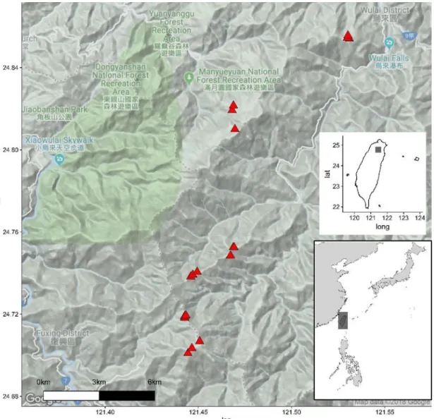
The study site is located in La-La Shan area in Northeast Taiwan (Figure 1), along

elevation gradient from Ba-Dao-Er Shan (low elevation limit) in Wulai (N 24°51'15.91",

E 121°31'47.86") to Ta-Man Shan (high elevation limit) in Fuxing (N 24°42'12.31", E

121°26'47.6"). Elevation range is between 850 m a.s.l to 2100 m a.s.l, study area is on the

margin of New Taipei City district and Taoyuan City district. Climate in this area is warm

and wet (Figure 2), with average annual temperature 16.1°C and average annual

Figure 1: Map of the study area.

(19)

precipitation 2070 mm. Mean monthly temperature for the coldest month (January) is

6.2 C and for the warmest month (July) is 24.8°C. This weather data were collected by

the closest weather station established by Central Weather Bureau (La-La Shan,

24°41'25.02" N, 121°24'14.1" E, elevation 1374 m a.s.l., data recorded from 2008 to

2017). According to geographical climatic regions distinguished by Su (1985), the study

area is on the boundary of Northeast and Northwest region. Types of geological substrates

are argillite, shale, slate, sandstone and phyllite (Central Geological Survey, MOEA). The

forest vegetation is represented by three types: high elevation Chamaecyparis montane Figure 2: Climatic diagram of La-La Shan station in La-La Shan.

(20)

mixed cloud forest, mid-elevation Quercus montane evergreen broad-leaved cloud forest

and low elevation Pyrenaria–Machilus subtropical winter monsoon forest (Li et al. 2013).

2.2 Sampling design

The sampling design has 18 400-m² and

60 100-m² plots, distributed into six

elevation zones－850, 1100, 1350, 1600,

1850 and 2100 m a.s.l. For 400-m² plots,

each elevation zone according to the

topography and monsoon direction, plots

were assigned into three groups－leeward, ridge and windward side. Windward side plots

faces northeast while leeward plots southwest direction. Each plot is a square 20 m×20 m

of total area 400 m². 100-m² plots are squared, 10×10 meters (area of 100 m²). Each

elevation has 10 100-m² plots, including three that are subplots of 400-m² plots.

According to their topographical position, 100-m² plots can be also classified into leeward,

ridge and windward. The schema of the sampling design is presented on Figure 3. Each

plot also has its own three-letter code, with the first letter for transect (L = La-La Shan),

the second letter for elevation zone (1 for highest and 6 for lowest), and the third letter

for aspect (L for leeward, R for ridge and W for windward). For example, L1W means Figure 3: Schema of sampling design.

(21)

the plot in the highest elevation zone (2100 m a.s.l.) facing the northeast direction

(windward).

2.3 Species abundance

In 400-m² plots, I surveyed the species composition and measured DBH of each

individual (only individuals with DBH ≥ 1 cm were recorded). Species abundance is

calculated using importance value index. The equation for calculating IVI of each species

is given by

IVI = (relative abundance+ relative basal area)/2 (eq. 1)

Relative abundance is calculated as number of individuals tree of one species at the plot

divided by the number of all individual trees at the plot. To calculate relative basal area,

I calculated basal area of each species. First, I used DBH to calculate basal area, as

(DBH/2)² of each individual. After that, the stem area of all individuals of the same

species was summed to get the basal area of that species. The basal area of each species

was divided by the sum of basal area of all individual trees in one plot to attain the relative

basal area of each species.

In the 100-m² plots, I surveyed the species composition (only individuals taller than

two meters were recorded) without measuring the DBH for each individual. I had totally

61 100-m²plots along the elevation gradient; all the elevation zones have 10 plots except

(22)

1600 m a.s.l. elevation zone has 11 plots. I chose the plots in which over 80 % of

individuals have measured trait values (one plot from the 2100 m elevation did not fit this

criteria, since it was dominated by coniferous species, and was removed from the

analysis). As a result, I used 60 100-m² plots to do analysis.

2.4 Environmental factors

We record geographical coordinates and took several photographs for recording the

situation for each plot when we did the survey. Geographical coordinates were recorded

by GPS (GARMIN GPSMAP 64st, USA).

2.5 Trait sampling

Between December 2016 and September 2018, I collected and measured traits of 215

broad-leaf tree individuals. I also used data from other 250 individuals which were

collected and measured in October 2014 in a previous project (Zelený & Li, unpublished

data). Because at that time was the beginning of the project, our lab collected the samples

to see the pattern. This study take the data from that to make database more complete.

Altogether, the database contains traits from 465 individuals belonging to 119 broad-leaf

tree species.

Individuals of dominant species taller than two meters were selected for the sampling.

(23)

If one species was very dominant at one plot, I chose one or two biggest trees for sampling.

Before collecting, I measured each tree’s diameter at breast height (DBH). For each

individual, I collected several twigs with at least six leaves for measuring leaf traits. I

collected leaves, which were growing on the top of the canopy and were exposed to full

sun. In order to collect leaves from the upper part of the canopy, I used telescopic knife

(used by farmers to collect betel nuts, longest length around 14 meters) to cut the branch

with several leaves, then I picked up the small twig with entire leaves. After collecting at

least six entire leaves, I put them into plastic zipper bags with moistened paper or toilet

tissue. Before transporting the samples back to laboratory, I put plastic bags in portable

cooler with ice if possible. After arriving at the laboratory, I put plastic bags in a

refrigerator of 4°C.

Wood samples were collected in two ways. For individuals with DBH larger than 10

centimeters, I used increment borer (SUUNTO Increment Borers, Finland) with 5.15mm

diameter and followed the method described by Chave (2006). Before taking the sample

core, I used knife to remove mosses and outer bark of the tree at around the breast height.

Then I sticked the borer inside the cleaned spot on the trunk, and keep turning the handle

of borer until it got into the stem. When borer reached half of the stem, I turned the handle

a little bit back to break the core inside the borer. I used the extractor part of the borer to

get the entire wood core out. I put the core into plastic straw, cut strew into appropriate

(24)

length and seal both ends of the straw with parafilm M. I wrote the individual code on the

straw and put it into plastic zipper bag. For the individuals with DBH less than 10

centimeters, I directly took their branches with diameter larger than 1 centimeter and

length around 15 centimeters. Arriving at laboratory, I put all wood samples in a

refrigerator of 4°C and prepared them for measuring.

2.6 Trait measurement

I measured 14 functional traits, including leaf area (LA), specific leaf area (SLA), leaf

dry-matter content (LDMC), leaf thickness (Lth), succulence, chlorophyll content (Chl),

leaf water repellency (Dropupper and Dropbelow), venation density (VD), wood density

(WD), stable isotope ratio of nitrogen and carbon of leaf (δ¹⁵N and δ¹³C) and content of

nitrogen and carbon per mass in leaf (Nmass and Cmass). If not stated otherwise, the

measurement methods followed the handbookof Pérez-Harguindeguy et al. (2013).

For the measurement of functional traits, branches with leaves enclosed in plastic

bags were taken out from the refrigerator. Six entire leaves, from the branch sampled from

the same individual tree without damaged by the insect or covered by mosses were cut

and their petioles removed. These leaves were separated into two groups, each group has

three leaves. I then put the leaf into two transparent folders as soon as possible to avoid

the leaves losing water. After I finished collecting three to five individuals, I put the

(25)

remaining samples and one other folder which contains the other three leaves back to the

refrigerator. Samples in a prepared folder were waiting for the follow-up measurements.

For each measurement I used three leaves from each individual.

2.6.1 Leaf morphology measurements

Leaf fresh weight was measured by an electric balance (OHAUS Adventurer AR2140,

USA) with precision of 0.0001 g. Leaf thickness (Lth) was measured by digital display

thickness gauge (DML digital thickness gauge, UK) with precision of 0.001 mm. Primary,

secondary or obvious tertiary veins were avoided during the measurement. Leaf thickness

at upper right, upper left, lower right and lower left of the lamina were measured and

averaged. Leaf area (LA) was estimated by a scanner (Perfection V370 Photo, EPSON).

I put three leaves on the screen of scanner, upper lamina facing down, avoiding individual

leaves to overlap. Petioles of the leaves were positioned to the same direction. A ruler 5

centimeters long was placed on the corner of the screen as a scale. The scan resolution

was set to 300 dpi. After the image was scanned, leaf area was estimated by ImageJ

program (Fiji), which is a freeware software. After leaf scanning, each lamina was put

into an envelope folded from newspapers. All leaf samples in envelopes were dried in the

oven at 70°C for three or more days, to make sure the leaf was dry. I used again the four-

digit scales weight to measure the dry weight (LDW) of the leaf.

(26)

Specific leaf area (SLA) was calculated as one-side leaf area divided by leaf dry

weight (LA/LDW). Leaf dry-matter content (LDMC) was calculated from leaf dry weight

divided by the fresh weight (LDW/LFW). Leaf succulence was calculated from leaf dry

weigh, leaf fresh weight and leaf area (Mantovani 1999). The equation is following:

Succulence = (Leaf fresh weight- Leaf dry weight) *1000 / Leaf area (eq. 2)

2.6.2 Chlorophyll content (Chlmass)

A chlorophyll meter (SPAD-502, KONICA MINOLTA, Japan) was used for the

measurement of leaf chlorophyll content. I divided lamina into two parts, left and right,

and for each part I took the measurement at three random points. The average of these six

measurements represents the chlorophyll content for each leaf. In the previous project,

the chlorophyll content was measured by a different instrument (CCM-200, APOGEE,

USA). Because I wanted to use values measured both by SPAD and CCM in the same

analysis, I calibrate values measured by these two instruments, I did a small test to convert

the value of CCM-200 to SPAD-502 (Appendix 1). According to the result, I used the

regression line as calibration equation. The equation of calibration is following:

SPAD = -12.85+log(CCM)х18.26 (eq. 3)

I also transfer the chlorophyll content measured by SPED to chlorophyll content per

mass (Chlmass). The equation is Chlmass= ((117.1*SPAD)/(148.84-SPAD))*SLA (Coste et

(27)

al. 2010).

2.6.3 Leaf water repellency (Dropupper and Dropbelow)

Remaining leaves which were not used for other trait measurement were used for

measuring leaf water repellency and venation density (VD). For leaf water repellency

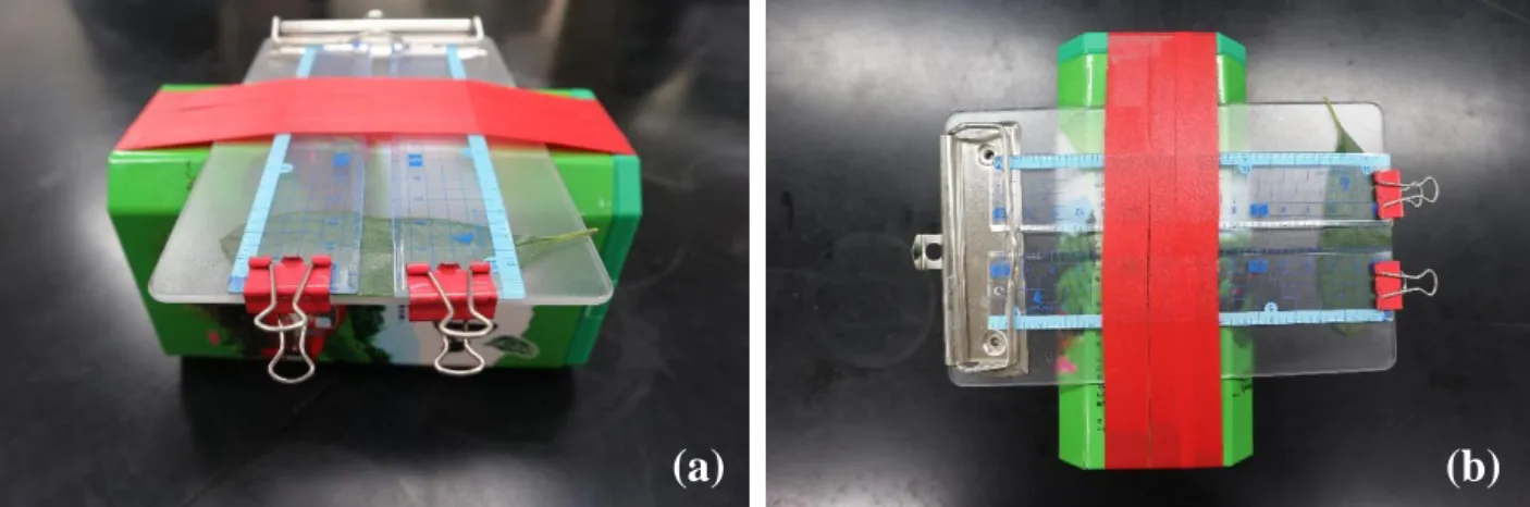
measurement, leaves were placed on flat custom-made platform (Figure 4) consisting of

one box (17.5 cm × 10 cm × 8 cm), one clipboard (10.6 cm × 18.5 cm), two rulers (around

12 cm) and four binder clips (two 32 mm and two 19 mm). I bounded the clipboard on

the box, using two bigger binder clips, and fixed the ruler on the clipboard from beside

and other two clip at the front side of the platform. Distance between two rulers was

around 0.7 cm. The following measurements were done for both adaxial (upper) and

abaxial (lower) surface of each leaf sample. Three leaves from each individual were

measured. The leaf was mounted horizontally between clipboard and rulers by binder

clips. One 5-μl droplet of distilled water was placed on the surface of lamina by a

micropipette (HIRSCHMANN labopette 2–20 μl single channel, Germany). Because

Figure 4: Platform for measuring droplet. (a) Front view (b) Top view

(a) (b)

(28)

droplet will spread and influence the angle of droplet, picture were taken as soon as

possible when water droplet was dropped on the leaf surface. Photos were taken by a

camera (NIKON D5500, Japan) equipped with lens (TAMRON SP AF 17-50 mm F2.8

XR Di II VC, Japan). Two or more photos for one treatment were taken. ImageJ (ImageJ

1.51u) with DropSnake plugin (Stalder et al. 2006) was used to analyze the photos. The contact angle (θ) was calculated following Aryal & Neuner (2010). Leaf surface was set

as the baseline, and the contact angle (θ) between a line at a tangent of the droplet running

through the point of contact between

the droplet and the leaf surface and

baseline was measured (Figure 5).

According to Crisp (1963), the leaves

with droplet angle higher than 110°

are considered as water repellent, and leaves with lower angle as not repellent.

2.6.4 Venation density (VD)

Leaves were cut into sections of 0.25–1 cm², with the section size depending on the size

of the original lamina. This section is located at the middle of the leaf and avoids primary

and secondary veins. Three sections from one individual (one section per leaf, three leaves

per individual) were measured. In order to make vein more visible, I used clearing method Figure 5: Determination of the contact angle (θ). Figure is modified from Fig.2 of Aryal

& Neuner (2010).

(29)

to make the section transparent. Sections from the same individual were put into a 20 ml

of Vials Scintillation Glass, containing 5% NaOH–H2O. The sections were soaked for

24–72 hours. Soaking time depends on the species. Leaves of some species need longer

time to become transparent. The transparent leaf sections were rinsed the leaf in distilled

water for several times. 1% safranin O in distilled water was transferred inside the Vials

staining the sections for 15 minutes. After staining, sections were rinsed again with

distilled water until no visible red color in the rinsed water. The sections were temporarily

mounted by water on the slide. I then used microscope (OLYMPUS CX31, Japan) to

observe the sections and used a CCD camera (MICROTECH HDC200, USA) to take

pictures. Several pictures were taken to complete one section. When all photographs were

finished, I used Image Composite Editor (2015 Microsoft Corporation, Version 2.0.3.0)

to assemble all pictures together. After these procedures, image for the analysis of

venation density was completed. The transect method applied by Blonder & Enquist

(2014) was then used to estimate the venation density. I randomly draw line segments on

vein image to get the parameter d (in equation 4), then counted the number of veins the

line crossed. Parameter d is calculated as the total length of a line (70 mm) divided by the

number of veins the line crossed. I calculated the vein density using the following

equation:

VD = 0.629 × (1/d) + 1.073 (eq. 4)

(30)

2.6.5 Wood density (WD)

Two approaches were used to estimate wood density. For wood core collected by the borer,

I directly took out the core from straw. If core broke into several segments, I removed the

segments shorter than 1 centimeter. For measuring the volume of the core, I used Archimedes’ principle with a box filled of 80% of water inside. The core segment was

inserted into water, and sink into water without touch the bottom of the box. The

increment of the weight represents the volume of this segment. After the volume being

measured, the segments were wrapped into aluminum foil and then dried in oven on

105°C for four to five days. Dry weight of the segments were measured on dried samples,

and wood density was calculated as volume divided by dry weight. For branch sample,

most of the steps were the same as those for the wood core. The bark of the branch was

removed before measuring its density.

2.6.6 Stable isotopes of leaf nitrogen and carbon content

Leafs from 160 individuals were analyzed for stable isotopes ratio. For each species, at

least one individual was analyzed. If this species occurs in more than one elevation zone

or is present in plots of all three of topography, I took more duplicates for analysis. Leaves

were ground into fine powder by mortar and pestle. Around two microgram of the powder

(31)

samples was weighted and wrapped into a tin capsule. The elemental analyzer (FlashEA

1112 series element analyzer, Thermo Fisher Scientific, Italy) was used to analyze carbon

(Cmass) and nitrogen (Nmass) contents. The ratio of stable carbon (δ¹³C) and stable nitrogen (δ¹⁵N) isotopes was measured with an isotope ratio mass spectrometer (Delta V

Advantage, Finnigan Mat, Germany). The stable isotopes ratio δ¹³C (or δ¹⁵N) is expressed

as: δ¹³C (or δ¹⁵N) = [(R sample/R standard) − 1]1000, where R sample is ¹³C/¹²C (or

15N/¹⁴N). The global standard for δ¹³C is PeeDee belemnite (PDB) and for δ¹⁵N is the

nitrogen in atmosphere.

2.7 Statistical analysis

Analysis was separated into two parts, trait-trait relationship and trait-environment

relationship. In order to make a normal distribution of all the traits, I log-transformed

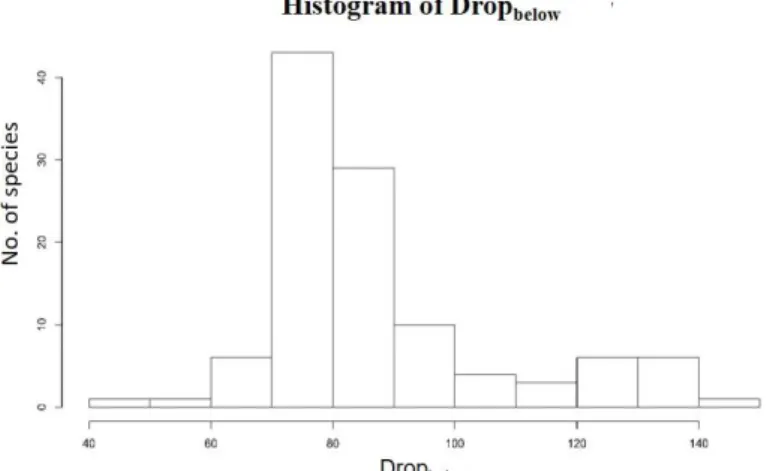
values of LA, SLA, Dropbelow and Nmass, and squareroot-transformed values of Lth,

Dropupper, Chlmass, succulence and VD, and took the cube for Cmass. I removed the leaf

water repellency for trait-trait

relationships, because this trait

much like to descript the

appearance of the leaf. It is

inferenced by the hair or wax on

Figure 6: Histogram of Dropbelow

(32)

the leaf surface. Species present on the right side of Figure 6 indicated the feature of hairy

leaf, i.e. Quercus gilva, Litsea elongata var. mushaensis and Rhododendron formosanum.

It’s not easy to compare the morphological traits to others, so I removed it.

For the analysis of the trait-trait relationship, I used principal component analysis

(PCA) and pairwise correlation test. I only chose 90 species which are present in my

species composition of transect for the trait-trait relationship analysis. I standardized all

the traits to zero mean and unit variance before I used PCA analysis. Due to PCA analysis

removes the whole sample which contains the missing value, I only used 78 species for

PCA calculation. Pairwise test was focused on the relation among each pair of traits. I calculated the Pearson’s correlation between traits, and tested the significance by t-test.

The intraspecific variance also calculated for species which is more than ten individuals

and shows in Table S1 (Appendix 2).

For trait-environment relationship, I analyzed both 400-m² plots and 100-m² plot.

Because some plots have big conifer species, I chose presence-absence data of the species

as the species composition to calculate the main results. I also calculated the trait-

environment relationship by IVI, and included results in the appendix. Although the

community weighted mean (CWM) is a common way to analyze the relationship between

traits and environment. CWM is less powerful than fourth-corner analysis; both CWM

analysis and fourth corner suffer from inflated Type I error rate, which is solved by max

(33)

text in both cases (CWM and fourth-corner). In order to avoid this artificial statistics

problems, the fourth-corner analysis (Legendre et al. 1997; Dray & Legendre 2008) is the

way I used to calculate the relationship between traits and environmental factor. The

significance was tested by max test (Cormont et al. 2011). Because the results of fourth-

corner are not easy to be visualized, I used CWM to visualize them. The fourth-corner

correlation coefficient is the same as the slope of regression line from weighted regression

analysis of CWM which is calculated from weighted-standardized traits and weighted-

standardized environment variable (ter Braak et al. 2018).

All my statistical analyses were done in R program (R 3.5.0). PCA analysis is based on “vegan” package. Trait-environment relationship was calculated using the “weimea”

package (Zelený 2018). The R code shows in Appendix 6.

(34)

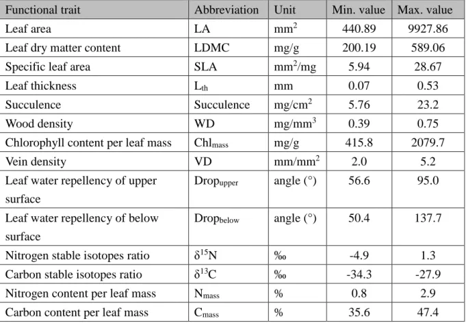
Table 1: List of traits measured in this study and maximum and minimum value of each trait.

Results

3.1 Values of traits

In this study, I measured 14 traits of dominant woody species in the plots. The maximum

and minimum values of the 14 traits are listed in Table 1. The values are within to the

range of values shown in Pérez-Harguindeguy et al. (2013).

Functional trait Abbreviation Unit Min. value Max. value

Leaf area LA mm² 440.89 9927.86

Leaf dry matter content LDMC mg/g 200.19 589.06

Specific leaf area SLA mm²/mg 5.94 28.67

Leaf thickness Lth mm 0.07 0.53

Succulence Succulence mg/cm² 5.76 23.2

Wood density WD mg/mm³ 0.39 0.75

Chlorophyll content per leaf mass Chlmass mg/g 415.8 2079.7

Vein density VD mm/mm² 2.0 5.2

Leaf water repellency of upper surface

Dropupper angle (°) 56.6 95.0

Leaf water repellency of below surface

Dropbelow angle (°) 50.4 137.7

Nitrogen stable isotopes ratio δ¹⁵N ‰ -4.9 1.3

Carbon stable isotopes ratio δ¹³C ‰ -34.3 -27.9

Nitrogen content per leaf mass Nmass % 0.8 2.9

Carbon content per leaf mass Cmass % 35.6 47.4

(35)

26

3.2 Trait-trait relationship

To investigate the relationship among and between traits, I only used 12 traits. Because

leaf water repellency is more an indicator of plant morphology, this trait is not used in the

trait-trait analysis.

3.2.1 PCA analysis of traits

Because trait data contain some missing values, PCA analysis removes the species that

include these missing values. As a result, PCA results are based on only 78 species. The

first axis explains 29.84 % of the variation in the data, the second 21.72 % and the third

12.64 % of the variation. The ordination diagram presents the relationship between them

and shows species scatter on ordination diagram (Figure 7 and Figure 8). The eigenvalue

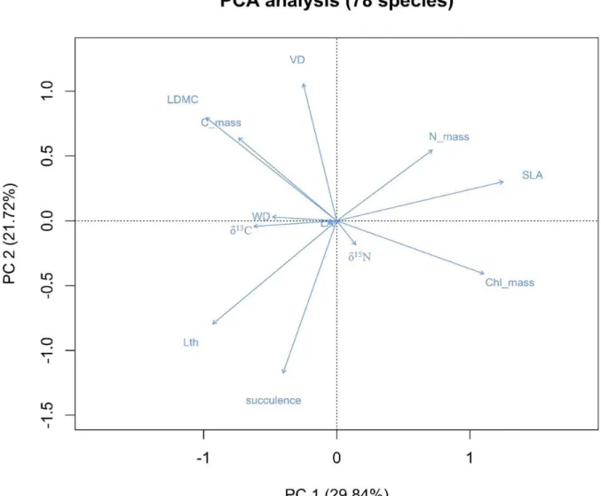
of each trait for first three axes is shown in Table S2. These 12 traits can be separated into

three groups (Figure 7). The first group contains SLA, LA, Lth, succulence, Chlmass, Nmass

and δ¹³C. SLA is positively correlated with Nmass and Chlmass. All these three traits are

negatively correlated to Lth, succulence and δ¹³C. The second group includes LDMC, VD,

WD and Cmass and are positively related to each other. Based on the Figure S2 (Appendix

3), δ¹⁵N is not correlated to other traits and belongs to the third group.

(36)

Figure 7: PCA diagram showing relationship between 12 traits calculated from 78 species. The first axis (PC1) explains 29.84% of variance, the second axis (PC2) explains 21.72% of variance.

(37)

28

Figure 8: PCA diagram showing relationship between 12 traits with species, calculated from 78 species. Species abbreviations are formed by two letters of genus and two letters of species name, all species names are listed in Appendix 4. The labels in corners indicate the strategy of each quadrant.

(38)

3.2.2 Relationship between traits

To reveal the relationship between traits, I examined the correlation between each pair of

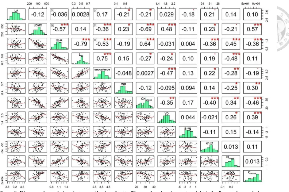
traits based on the species level (Figure 9). When considering only significant

relationships (p < 0.05), the results show that SLA is correlated with several other traits:

negatively with LDMC, Lth, succulence, chlorophyll, δ¹³C and Cmass, while positively

with Nmass. LDMC is negatively correlated with succulence, positively correlated with

VD and Cmass. Succulence is positively correlated with Lth and chlorophyll, and negatively

with VD and Nmass. VD is positively correlated with Cmass. δ¹⁵N is the only trait which is

not correlated with other traits. The pairwise relationship which is marked by ※ on Figure

9 indicates that these two traits are not independent. For example, both succulence and

LDMC contain leaf dry weight and leaf fresh weight in their calculation (succulence =

(leaf fresh weight – leaf dry weight)/leaf area, LDMC = leaf dry weight/leaf fresh weight)

thus, these two traits are not independent. The significant relationship between two

variables which are not independent should be interpreted with care, because they are a

case of spurious correlation between two not-independent variables (Brett 2004).

(39)

30

Figure 9: Diagram of correlations between all pairs of traits. The number showing on top right is the Pearson’s correlation coefficient between two traits. Symbols represent different level of p-value (*** = p < 0.001, ** = p < 0.01,

* = p < 0.05, · = p < 0.1, ※ = these two factors are non-independent variables).

(40)

3.3 Trait-environment relationship

I calculated the relationship between traits and environmental variable using the fourth-

corner analysis. Because the results of the fourth-corner analysis are not easy to visualize,

I used community weighted mean (CWM) to visualize them. Regarding the p-values, I

interpreted results with p < 0.05 as significant, p < 0.1 as marginally significant, and

p < 0.2 as having trend which is not significant, but worth to be mentioned.

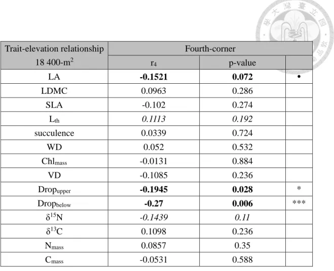
3.3.1 The fourth-corner analysis of 18 400-m² plots

The relationship between traits and elevation gradient was analyzed also for data from

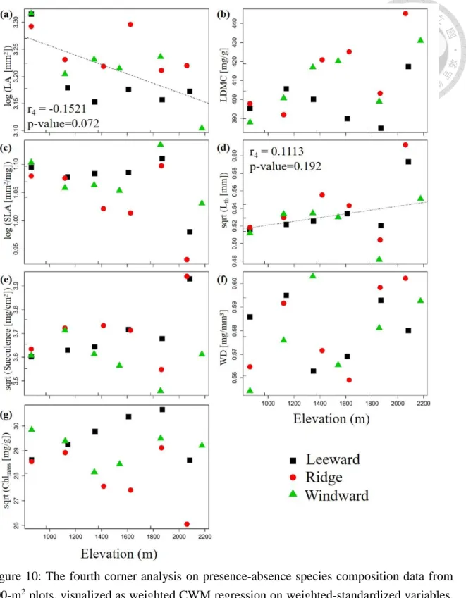
the survey of the 18 400-m² plots (Figure 10). I tested the significance of the relationships

using the fourth-corner analysis (Table 2). Results show that both LA and leaf water

repellency are negatively significantly related to elevation (p < 0.1). δ¹⁵N also shows the

negative trend along elevation (p = 0.11). Although other traits did not show significant

pattern along elevation, SLA and VD has decreasing trend with elevation. For some traits,

the differences in CWM values among leeward, ridge and windward plots increase with

elevation (e.g. LA, SLA, Lth and δ¹⁵N; Figure 10). According to Figure S3 and Table S3,

the pattern is similar to presence-absence data when use IVI value as the species

composition data to do the fourth-corner analysis. The only difference is the presence of

the positive trend in Chl (p = 0.194) and in δ¹³C (p = 0.066) along the elevation.

(41)

32

Figure 10: The fourth corner analysis on presence-absence species composition data from 400-m² plots, visualized as weighted CWM regression on weighted-standardized variables.

Individual panels show the elevation pattern of a) LA, b) LDMC, c) SLA, d) Lth, e) succulence, f) WD, g) Chlmass, h) VD, i and j) leaf water repellency, k) δ¹⁵N, l) δ¹³C, m) Nmass

and n) Cmass. r4 is the fourth corner correlation coefficient, p-value is the significance calculated by max test. The significant regression (p<0.05) is displayed by solid regression line, marginally significant (p < 0.1) by dashed line, and non-significant but worth to mention (p < 0.2) by dotted line.

(42)

Figure 10: continuation

(43)

34

Table 2: The result of fourth-corner analysis which tests the relationship between traits and elevation gradient, using 18 400-m² plots and presence-absence species composition data. r4 is the fourth corner correlation coefficient between traits and elevation. (*** = p < 0.001, ** = p < 0.01, * = p < 0.05, ˙ = p < 0.1. Values printed in bold are significant or marginally significant (p < 0.1), italics indicate results worth to mention with 0.1 ≤ p < 0.2)

Trait-elevation relationship 18 400-m²

Fourth-corner

r4 p-value

LA -0.1521 0.072 ˙

LDMC 0.0963 0.286

SLA -0.102 0.274

Lth 0.1113 0.192

succulence 0.0339 0.724

WD 0.052 0.532

Chlmass -0.0131 0.884

VD -0.1085 0.236

Dropupper -0.1945 0.028 *

Dropbelow -0.27 0.006 ***

δ¹⁵N -0.1439 0.11

δ¹³C 0.1098 0.236

Nmass 0.0857 0.35

Cmass -0.0531 0.588

(44)

3.3.2 The fourth-corner analysis of 60 100-m² plots

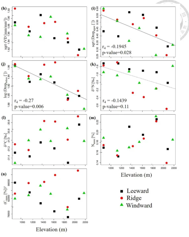
The relationship between traits and elevation are showed on Figure 11. Results of the

fourth-corner analysis are presented in the Table 3. LA, leaf water repellency and δ¹⁵N

are negatively correlated with elevation. LDMC is positively correlated with elevation.

SLA and Lth are on the margin of the significance (p < 0.1) and positively correlated to

the elevation. Similar to the pattern formed on 400-m² plots the variability of CWM

values is low in low elevation plots, while that is high in high elevation (e.g. LA, LDMC,

SLA, Lth, leaf water repellency and δ¹⁵N). Some traits group together according to

leeward, ridge and windward plots in high elevation (e.g. SLA, Lth, succulence, Dropbelow

and Nmass). The results from the fourth corner analysis using IVI species composition data

are almost the same as the result using the presence-absence data (Figure S4 and Table

S4).

(45)

36

Figure 11: The fourth corner analysis on presence-absence species composition data from 100-m² plots, visualized as weighted CWM regression on weighted-standardized variables.

Individual panels show the elevation pattern of a) LA, b) LDMC, c) SLA, d) Lth, e) succulence, f) WD, g) Chl, h) VD, i and j) leaf water repellency, k) δ¹⁵N, l) δ¹³C, m) Nmass

and n) Cmass. r4 is the fourth corner correlation coefficient, p-value is the significance calculated by max test. The significant regression (p<0.05) is displayed by solid regression line, marginally significant (p<0.1) by dashed line, and not significant but deserving attention (p<0.2) by dotted line.

(46)

Figure 11: continuation

(47)

38

Table 3: The result of fourth-corner analysis which is tests the relationship between traits and elevation gradient, using 60 100-m² plots and presence-absence species composition data. r4 is the fourth corner correlation coefficient between traits and elevation. (*** = p < 0.001, ** = p < 0.01, * = p < 0.05, ˙ = p <0.1, italics indicate that 0.1 < p < 0.2). Values printed in bold are significant or marginally significant (p

< 0.2).

Trait-elevation relationship 60 100-m²

Fourth-corner

r4 p-value

LA -0.2179 0.036 *

LDMC 0.1955 0.066 ˙

SLA -0.1657 0.11

Lth 0.1359 0.164

succulence -0.01 0.918

WD 0.0735 0.492

Chlmass -0.1142 0.294

VD -0.0375 0.728

Dropupper -0.2233 0.018 *

Dropbelow -0.2795 0.002 **

δ¹⁵N -0.1956 0.066 ˙

δ¹³C 0.0788 0.46

Nmass 0.0695 0.544

Cmass -0.0328 0.788

(48)

Discussion

Functional traits are useful for understanding the adaptations of plants along the

environmental gradients (Violle et al. 2007). In this study, I measured 14 traits of woody

species to evaluate how plant community adapts along the elevation gradient. In order to

understand how elevation influence community composition, I used trait-trait relationship

to classify the growth strategy. Then, I used trait-environment relationship to see which

traits are correlated with the elevation gradient. Results of these two relationship can

provide information for how environmental filters determine community composition by

acting on traits.

4.1 Trait-trait relationship

I referenced previous studies and chose 14 traits (Wright et al. 2004; Lavorel et al. 2007).

But trait-trait relationships were commonly observed, it’s not necessary that these

relationships exist everywhere (Wright et al. 2005). The pattern of trait-trait relationship

may differ among studies due to different environmental conditions. The trade-off

between traits might be different in my study.

Classification of traits into groups is helpful for us to understand how traits influence

the plant fitness. It also provides a tool to simplify the measurement for future studies

through focusing on the main features and to improve the efficiency of the study. Study

(49)

40

effort can be reduced by avoiding measuring redundant traits. I grouped traits mostly

based on the PCA analysis (Table S2), but also did some modification according to the

results of pairwise correlation (Figure 9).

4.1.1 Traits related to leaf economic spectrum

First group includes SLA, Lth, succulence, chlorophyll content per mass (Chlmass), Nmass, LA and δ¹³C. SLA was shown to be significantly related to leaf nitrogen concentration

and carbon investment (Wright et al. 2004). SLA is a compound trait to describe different

life strategies. Result of the trait-trait pairwise correlation plot (Figure 9) shows that SLA

is highly correlated with other traits, including LDMC, Lth, Chl, δ¹³C, Nmass and Cmass.

Therefore, I consider traits without SLA to define this group. Chlorophyll content usually

has correlation with photosynthetic rate (Kura-Hotta et al. 1987), and is positively related

to photosynthetic capacity (Muraoka & Koizumi 2005). Result of pairwise correlation

plot (Figure 9) shows that, Chlmass is correlated with Lth. It has been shown that Lth is

highly correlated with photosynthetic capacity (Mendes & Marenco 2010). This group

also includes nitrogen concentration per leaf mass (Nmass). Nmass is positively correlated

with photosynthesis and chlorophyll content (Ripullone et al. 2003). Succulence is

positively significantly correlated with Lth, and represents similar function. Succulence is

usually considered as a water-related trait of plants. Because succulence affects water

(50)

storage capacity, it might also influence photosynthetic gas exchange (Zhang et al. 2015).

SLA, Lth, succulence, Chlmass and Nmass are correlated with photosynthesis.

According to species distribution in the ordination diagram (Figure 8), deciduous species,

Acer morrisonense (臺灣紅榨槭) and Viburnum sympodiale (假繡球), have high values

of SLA and Nmass. Deciduous species usually have higher photosynthetic rate than

evergreen species (Yamori et al. 2014). The ordination diagram indicated that species with

high SLA, LA, Chlmass and Nmass are more acquisitive. High Lth and succulence species

are more conservative. Mendes & Marenco (2010) and Zhang et al. (2015) showed that

leaf thickness and succulence are positively correlated with photosynthetic rate. However,

my data show opposite result, which may be associated with mesophyll layer. It has been

reported that resistance of mesophyll can limit photosynthesis (Flexas et al. 2012). The

species in my data set may have thick mesophyll tissue and limit CO2 diffusion. In this

situation, photosynthetic rate is limited by mesophyll conductance (Evans et al. 2009).

δ¹³C can be used to identify photosynthetic pathways of the plant (Dawson et al. 2002).

The measured δ¹³C values of sampled species vary from -34‰ to -27‰. It indicates that

all of the sampled species used C3 pathway for photosynthesis. In C3 plants, δ¹³C is also

an indicator of photosynthetic WUE (Saurer et al. 2004). Species with higher δ¹³C have

higher WUE and generally have better tolerance for drought. LA influences the extent of

interception of radiant energy, absorption of CO2 and transpiration water lost. Leaf area

(51)

42

was also found to be correlated with the WUE (Markesteijn et al. 2011). Leaves of small

LA is the characters of the drought tolerant species.

The traits of this group are related to the photosynthesis and WUE. SLA, Chl, Lth

and Nmass are related to photosynthetic rate. LA, succulence and δ¹³C are related to WUE.

These traits describe conservative and acquisitive stategy of plant growth (de la Riva et

al. 2016). Accordingly, I define this group of traits as “leaf economic spectrum”

dimension.

4.1.2 Traits related to mechanical support

The second group includes LDMC, VD, WD and Cmass. LDMC is related to nutrient

concentration of nitrogen content and carbon-nitrogen ratio (Domínguez et al. 2012). It

is also a good proxy for physical anti-herbivore defenses (Wilson et al. 1999). Higher

LDMC means that plant invests more resource to leaf construction and produce more

rigid leaf. VD also influence two functions of plant i.e. resources transport and

mechanical support. VD represents the density of xylem in a leaf, which can transport

nutrients and water for photosynthesis, and the density of phloem, transporting the

product of photosynthesis and signal molecules. VD also provides mechanical support of

the lamina. These two functions are partially partitioned by order of the venation. Main

and second order veins provide mechanical support, third and minor vein focus on

(52)

nutrient transport (Sack et al. 2012). Wood is related to mechanical support, water

transport and storage capacity (Chave et al. 2009). It is also related to biomass allocation

(Mensah et al. 2016). LDMC, WD and VD are positively correlated with nutrient

allocation and mechanical support. Leaf Cmass indicates how much carbon was invested

by the plant to build the tissue of leaves. Leaves with higher carbon content indicate more

expensive tissue and tend to have longer life span. The leaves with higher Cmass and

LDMC also have slower decomposition rate among evergreen species (de Paz et al. 2017).

WD has been found to be related with biomass allocation (Mensah et al. 2016). Although

these four factors are associated with nutrient allocation and mechanical support, I only

choose one suitable description for this strategy. I defined this strategy based on the

species ordination diagram (Figure 8). Ordination diagram displays that Litsea acuminata

(長葉木薑子) and Carpinus rankanensis (蘭邯千金榆) are high LDMC, VD and Cmass

species. Carpinus rankanensis is only present at the windward plots facing strong wind

disturbance. This environmental disturbance may favor species which have rigid leaves

with dense vein (Anten et al. 2010). Litsea acuminata grows long leaves. Because longer

leaves are easily damaged by disturbance, they tend to increase LDMC for steadying the

flexural rigidity of the lamina (Vernescu & Ryser 2009). Based on these reasons, I define

this strategy as the mechanical support.