國立臺灣大學電機資訊學院電機工程學系 碩士論文
Department of Electrical Engineering
College of Electrical Engineering and Computer Science National Taiwan University
Master Thesis
利用色彩資訊及深度資訊之室內行動機器人 對行人偵測與追蹤
Pedestrian Detection and Tracking with Indoor Mobile Robot Using both Color Information and Distance
Information
林俊榮 Jun-Rong Lin
指導教授:連豊力 博士 Advisor: Feng-Li Lian, Ph.D.
中華民國一百零三年七月
July 2014
誌謝
即將要畢業,在研究所的兩年收穫良多。一路上的研究走來,首先要感謝的 就是我的指導教授連豊力博士,在這嚴謹的研究態度以及看待事情的觀點使得我 這兩年有很大的收穫。研究一個問題時,我終於懂得如何去定義一個問題、提出 想法並且去解決這個問題。以及在這些複雜的研究問題上,如何用有效率的簡報 讓大家了解,是我這兩年的成長。在口試時,感謝三位口試委員簡忠漢博士、李 後燦博士及黃正民博士提供許多的建議,使得這本論文可以更加完整。
感謝 NCSLabers 的大家,由於你們的陪伴,才能讓我這麼順利的將研究完 成。感謝志明學長,在研究遇到問題時,總是提供給我一些解決問題的想法。感 謝意淳學姊,在我的研究上,總是會敘述一些我沒有想到的研究盲點。感謝俊兆 學長,在研究上以及生活上,都受到你不少的幫忙。感謝飛紘學長,你每次說話 的梗總是很好笑,研究上也會提供我閱讀論文的訣竅。感謝中易學長,你每次總 會有出人意表的表現,而且在研究上甚至幫助我許多。感謝凱翔學長,每次都不 言其煩的跟我討論研究的事情,並且製造很多實驗室的歡樂。感謝柏逸,在我遇 到研究與生活瓶頸時,會與我一起討論。感謝家維,高等機器人學課程跟你討論 讓我學習很多。感謝兆良,你生活上的率性,研究上獨特的想法都值得我去學習。
感謝詠政,你在研究上的積極,以及生活上相處都是讓我值得效法。還有這一年 相處過來的學弟們。感謝孝淇,在我的研究上會適時給我鼓勵,並且全力提供協 助我。感謝登翔,在研究方面提供我一些想法,生活上的一些資訊也都會不吝的 提供。感謝鍾潛,有時候在做實驗時還會麻煩到你,並且提供我做實驗時可以有 不同的方式去表達。感謝博旭,你總是一個冷面笑匠,在研究中也是一位高深莫 測的人。感謝偉哲,有些時候會跟你借 Matlab 書籍來參考,以及和你討論一些 新想法。很開心可以在這間實驗室度過研究所生涯,少了你們其中一個,研究的 生活就會變了調。
最後,感謝我的家人。爸爸、媽媽、姊姊以及哥哥。有你們陪著我、包容我,
這研究的路才能夠如此順遂。未來的日子,我會繼續努力。在此,謹以此論文奉 獻給予所有的有緣人,如果有提供給你們任何想法,這就是我的榮幸。
林俊榮 謹誌 中華民國一○三年九月十九日
i
利用色彩資訊及深度資訊之室內行動機器人對行人偵 測與追蹤
研究生:林俊榮 指導教授:連豊力 博士
國立臺灣大學 電機工程學系
摘要
生活之中,人機互動是一門重要的學問。如果機器人可以隨時隨地去跟人互 動,那麼在生活上必定會便利不少。其中與人互動的情況中,追蹤行人就是其中 一個必須研究的課題。機器人追蹤行人的問題,主要分成兩類:自我定位與地圖 建構、行人偵測與追蹤。這些問題都是在做機器人追蹤行人時會碰到的項目。
以自我定位與地圖建構來說,要在未知路徑的情況下,得到行動機器人周邊 及本身存在的資訊是一件困難的事。在本篇論文裡,主要解決行動機器人編碼器 的硬體因素造成殘存誤差。利用粒子群最佳化演算法去找出更準確的機器人位置,
然後利用這些資訊可以估測出機器人周遭環境地圖。由於雷射測距儀是一個相當 精確的儀器,所以得到的距離資訊準確度是很高,在實驗部分會有驗證。在得到 行動機器人的位置和周遭地圖之後,就可以分辨出靜態物地圖和動態物地圖。對 行動機器人而言,是非常有用的資訊。然而,動態物的地圖推測會有一些問題,
ii
這部分會在論文中詳細的描述到。
另外,在行人偵測部分,除了用雷射測距儀所得到的動態點之外,也可以用 點的分群、大小以及資料可信度去判斷。另外,色彩資訊的添加可以當成是一個 更強韌的條件。偵測邊緣形狀的霍式圓形轉換、色彩判定以及頭的所在位置都是 偵測行人的準則。利用這些準則,幾乎可以更精確的去判斷行人。基於行動機器 人追蹤,由於追蹤目標行人在生活環境中可能會有靜態障礙物擋住或者附近突然 出現的行人,造成雷射測距儀的資料誤判。場景設定是在一般研究室或宿舍,通 常人的穿著色彩分佈及紋理分佈會不盡相同,所以可以透過色彩資訊去加以判斷。
並且使用距離資訊空間連續性去做一個強韌性判斷的準則。利用這些準則,就可 以強韌地去判斷行人,並且去做目標行人的追蹤。在本篇論文中,最主要的就是 用色彩資訊去解決在使用雷射測距儀時,行人偵測的判斷以及突然出現的人進而 造成追蹤判斷的錯誤。
在實驗結果顯示出在這些環境當中,可以解決雷射測距儀資料連結的不足,
並且可以做到追蹤目標行人。
關鍵字:雷射測距儀、全向攝影機、機器人自我定位、動態物偵測、行人偵測、
行人追蹤。
iii
Pedestrian Detection and Tracking with Indoor Mobile Robot Using both Color Information and Distance
Information
Student: Jun-Rong Lin Advisor: Dr. Feng-Li Lian
Department of Electrical Engineering National Taiwan University
ABSTRACT
In daily life, that mobile robot communicates with pedestrian needs many tasks.
The applications are used in guided vehicle, shopping cart, or office assistance. In this thesis, the tasks include self-localization, mapping, pedestrian detection, and target pedestrian tracking in unknown indoor environment.
To do self-localization and mapping, the accurate odometry of mobile robot is important. However, skidding and slipping can induce that the odometry is not equal to the real distance. In this thesis, particle swarm optimization (PSO) algorithm correct odometry in unknown indoor environment. The combination of the self-localization and the mapping is referred to as the simultaneous localization and mapping (SLAM) [39: Birk & Carpin 2006]. In the SLAM, once odometry of mobile robot is known, building a map is also a task which can be effectively solved at the
iv
same time [39: Birk & Carpin 2006]. Afterward, moving object detection is based on the precise map.
After the moving objects are detected, the next steps are pedestrian detection and target pedestrian tracking. In the pedestrian detection, the color image is regarded as an additional condition for the judgment based on the laser range finder (LRF) scan.
In target pedestrian tracking, owing to pillars hindering or new pedestrians appearing, the data association may be error between two consecutive LRF scans. In this thesis, a method based on color distribution and color texture to track pedestrian in color images is proposed. The experiment demonstrates the target pedestrian in the new pedestrian appearing and the pillars hindering. Through the experiments, the performance of pedestrian detection and target pedestrian tracking is not good.
However, the performance of pedestrian in color image is low owing to the resolution.
In the future, the detection and tracking moving object (DATMO) with LRF scan in Chapter 3 can combine the pedestrian detection and target pedestrian tracking with color image in this thesis.
Keywords: laser range finder, omnidirectional camera, robot self-localization,
moving objects detection, pedestrian detection, target pedestrian tracking.
v
Contents
摘要... i
ABSTRACT ... iii
Contents ... v
List of Figures ... vii
List of Tables ... xi
Chapter 1 Introduction ... 1
1.1 Motivation ... 1
1.2 Problem Formulation ... 3
1.3 Contribution ... 7
1.4 Organization of the Thesis ... 8
Chapter 2 Literature Survey ... 9
2.1 Simultaneous Localization and Mapping ... 9
2.2 Pedestrian Detection and Tracking ... 11
Chapter 3 Simultaneous Localization and Mapping ... 14
3.1 Laser Range Finder Usage and Limitation ... 15
3.1.1 Introduction of Laser Range Finder ... 15
3.1.2 The Limitation of Usage in the Glass Environment ... 16
3.2 Robot Localization ... 17
3.3 Map Construction... 21
3.3.1 Grid Map Construction ... 22
3.3.2 Static Map and Dynamic Map ... 23
Chapter 4 Pedestrian Detection and Target Pedestrian Tracking ... 26
4.1 The Operation Principle of Omnidirectional Camera ... 27
4.1.1 Introduction of Omnidirectional Camera ... 27
4.1.2 The Lightness of Omnidirectional Camera ... 28
4.2 Sensors Calibration ... 31
4.2.1 The Description of Calibration ... 32
4.2.2 Break Point and Angular Point Detection ... 33
4.2.3 Vertical Line Detection ... 35
4.2.4 Data Association ... 41
4.3 Pedestrian Detection ... 43
4.3.1 Pedestrian Detection Preprocessing with Laser Range Finder ... 43
4.3.2 Lower Line of Bounding Box Extraction ... 47
4.3.3 Upper Line of Bounding Box Extraction ... 52
4.3.4 Pedestrian Points Filtering in Static Map Construction ... 55
vi
4.4 Target Pedestrian Tracking ... 57
4.4.1 Color Distribution ... 57
4.4.2 Local Binary Patterns ... 58
4.4.3 Bhattacharyya Distance ... 59
4.4.4 Database Update ... 61
Chapter 5 Experimental Results and Analysis ... 62
5.1 Hardware Platform ... 62
5.2 Accuracy of Sensor Measurement ... 64
5.2.1 Laser Range Finder Accuracy ... 64
5.2.2 Sensors Calibration ... 72
5.3 Static and Dynamic Map ... 83
5.3.1 The Algorithms of Localization ... 83
5.3.2 The Map Construction ... 85
5.3.3 The Dynamic Map ... 87
5.4 Localization Accuracy ... 91
5.5 Pedestrian Detection Performance ... 96
5.5.1 Lower Line of Bounding Box ... 96
5.5.2 Pedestrian Map... 102
5.5.3 The Detection Accuracy ... 105
5.6 Target Pedestrian Tracking Performance ... 107
5.6.1 The Tracking Results and Accuracy ... 107
5.6.2 The Tracking Results and Accuracy ... 110
Chapter 6 Conclusions and Future Works ... 113
6.1 Conclusions ... 113
6.2 Future Works ... 114
References ... 116
Appendix ... 123
A.1 Distance Convert Pixel... 123
A.2 Lower Line of Bounding Box Extraction ... 126
vii
List of Figures
Figure 1.1 The Scene Shows the Pillars in the Indoor Environment. ... 3
Figure 1.2 Dynamic Environment with Pillars Occlusion ... 5
Figure 1.3 Dynamic Environment with New Pedestrian Appearing Nearby ... 5
Figure 2.1 Simultaneous Localization and Mapping Categories ... 11
Figure 2.2 Pedestrian Detection and Target Pedestrian Tracking Categories ... 13
Figure 3.1 The Operation Principle of Laser Range Finder ... 16
Figure 3.2: The Texture Influence in Glass Environment ... 17
Figure 3.3 The Illustration and Process of Particle Selection ... 19
Figure 3.4 Scan Matching 2 Data Result ... 21
Figure 3.5 The Inverse Observation Model Problem ... 25
Figure 4.1 The Omnidirectional Camera Structure ... 28
Figure 4.2 The Light Depends on the Active Lighting Source ... 29
Figure 4.3 Display Image with Lightness Problem in Ming-Da Building 2F ... 30
Figure 4.4 Each Variable in Histogram Equalization ... 31
Figure 4.5 Calibration Problems: Horizontal Adjustment, Translation, and Rotation . 33 Figure 4.6 The Break Points and Angular Points ... 34
Figure 4.7 The Flow Chart of Projection Center Search ... 36
Figure 4.8 Results of the Projection Center Search Algorithm ... 37
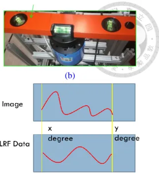
Figure 4.9 The Idea Process of Panorama Image... 38
Figure 4.10 Real Scene Image Process in Ming-Da Building 5F ... 38
Figure 4.11 The Sobel Vertical Edge Detector ... 40
Figure 4.12 The Example of Two Image for Sobel Vertical Edge Detector ... 40
Figure 4.13 The Process of Vertical Line Detection ... 40
Figure 4.14 Vertical Edge Detector in the Same Threshold Value ... 41
Figure 4.15 The Data Association Conception Matching the Feature Points ... 42
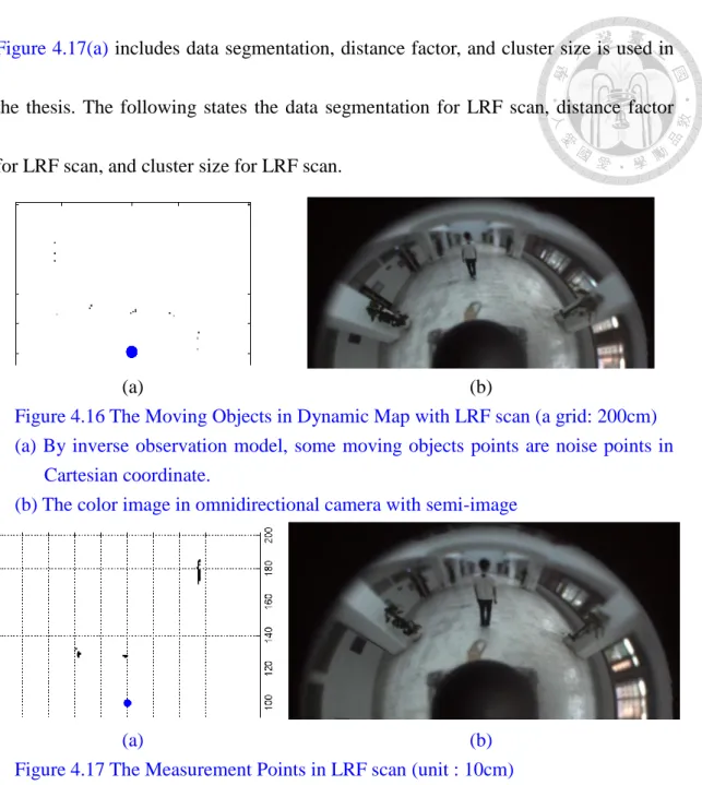
Figure 4.16 The Moving Objects in Dynamic Map with LRF scan ... 44
Figure 4.17 The Measurement Points in LRF scan ... 44
Figure 4.18 The Data Segmentation Result in LRF scan ... 45
Figure 4.19 The Distance Factor in LRF Scan ... 46
Figure 4.20 The Cluster Size of Elimination in LRF Scan ... 46
Figure 4.21 The Omnidirectional Camera Model ... 48
Figure 4.22 The Hyperbolic Surface Extraction ... 48
Figure 4.23 The Curve Fitting of SVD algorithm ... 49
Figure 4.24 The Omnidirectional Camera Model with Pedestrian Estimation in Omnidirectional Camera Image Pixel from Projection Center ... 50
viii
Figure 4.25 The Ground Bounding Box Result Demonstration ... 51
Figure 4.26 The Left Line, the Right Line, and the Lower Line of Bounding Box. .... 52
Figure 4.27 The Hough Circle Transform ... 54
Figure 4.28 Test of Pedestrian Detection ... 55
Figure 4.29 Pedestrian Points Filtering Process ... 56
Figure 4.30 The Example for LBP Operator ... 59
Figure 4.31 The Bhattacharyya Distance Coefficient Illumination ... 60
Figure 5.1: The Experimental Instrument ... 63
Figure 5.2 The Experimental Mobile Robot ... 64
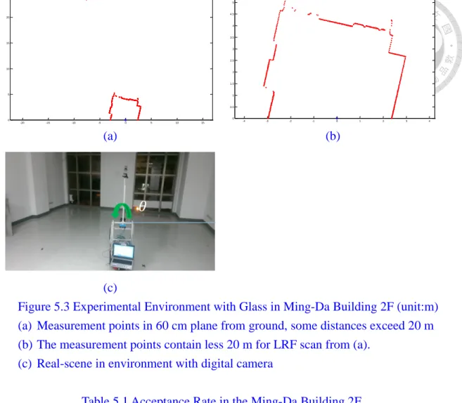
Figure 5.3 Experimental Environment with Glass in Ming-Da Building 2F ... 66
Figure 5.4 Plot the Acceptance Rate with Each Angle in the Table 5.1 ... 66
Figure 5.5 Experimental Environment in Ming-Da Building Lab 601 ... 67
Figure 5.6 Data Number of Sampling with Error Percentage Analysis ... 68
Figure 5.7 The Measurement Points of the LRF Scans ... 70
Figure 5.8 Plot the Acceptance Rate Result with Each Angle in Table 5.2 ... 71
Figure 5.9 Errors with Equation (5.1) and Equation (5.2) ... 71
Figure 5.10 The Break Points and Angular Points with LRF Data ... 73
Figure 5.11 The classification represents the break point ‘∗’ and the angular point ‘o’. ... 74
Figure 5.12 The Position of the Omnidirectional Camera ... 75
Figure 5.13 The Process in Finding the Projection Center ... 75
Figure 5.14 The Panorama Image from Omnidirectional Camera... 76
Figure 5.15 The SHL Extraction Method from Omnidirectional Camera ... 77
Figure 5.16 The analysis of Figure 5.15 ... 78
Figure 5.17 The Sobel Vertical Edge Detector for Ming-Da Building 6F ... 79
Figure 5.18 (a)~(f) The Distance Converts the Pixel ... 81
Figure 5.19 The Curve Fitting in Table 5.5 ... 82
Figure 5.20 The Robotic Position with Encoder with Different Path ... 84
Figure 5.21 The Localization with the Odometry, the ICP Algorithm, and the PSO Algorithm in the Three Cases. ... 85
Figure 5.22 The Map Construction by the Occupancy Grid Map and PSO Algorithm ... 87
Figure 5.23 The State from Free to Occupancy in Pedestrian Walk ... 89
Figure 5.24 The State from Unknown to Occupancy in Pedestrian Walk ... 90
Figure 5.25 The Experimental Scene in Ming-Da Building 4F ... 91
Figure 5.26 The Measurement Center of Robot Points for Ground Truth ... 92
Figure 5.27 The Location of Each Results in Ming-Da Building 4F ... 93
Figure 5.28 The Error Mean of each Scan Matching with Ground Truth Difference .. 94
ix
Figure 5.29 The Location of Each Results in Ming-Da Building 4F ... 95
Figure 5.30 The Error of each Scan with Ground Truth ... 96
Figure 5.31 The Calibration of Omnidirectional Camera in Digital Camera Image ... 97
Figure 5.32 The Omnidirectional Camera Hyperbolic Surface ... 99
Figure 5.33 The Height Convert Pixel in Ming-Da Building 4F ... 100
Figure 5.34 The Mean and Standard Difference in Table 5.10 ... 101
Figure 5.35 The Scene illumination with Laser Range Finder and Omnidirectional Camera ... 102
Figure 5.36 The Candidates in Dynamic Map ... 103
Figure 5.37 The Hough Circle Transform for Each Candidate ... 104
Figure 5.38 The Illustration of Receiver Operating Characteristic ... 105
Figure 5.39 Tracking Target Results in Case I from Figure 5.34(a) ... 109
Figure 5.40 Tracking Target Results in Case II-1 from Figure 5.34(b) ... 110
Figure 5.41 Tracking Target Results in Case II-2 from Figure 5.34(b) ... 110
Figure A.1 (a)~(t) The Distance Converts the Pixel (From Figure 5.18) ... 125
Figure A.2 The Height Convert Pixel in Difference Height (From Figure 5.33) ... 129
x
xi
List of Tables
Table 3.1 The Occupancy Probability of Each State S ... 23
Table 3.2 Inverse Observation Model ... 24
Table 5.1 Acceptance Rate in the Ming-Da Building 2F ... 66
Table 5.2 Acceptance Rate in the NCSLab in 100 data ... 70
Table 5.3 Properties of Laser Range Finder ... 72
Table 5.4 Projection Center Search ... 76
Table 5.5 The Distance Data and The Pixel Data ... 82
Table 5.6 The Rotation Angle with Each Feature ... 83
Table 5.7 The Error of Each Algorithm with Ground Truth in Figure 5.26 ... 93
Table 5.8 The Error of Each Algorithm with Ground Truth in Figure 5.28 ... 95
Table 5.9 The Camera Intrinsic Parameter ... 98
Table 5.10 The Results in Figure A.2... 101
Table 5.11 The ACC of detection with new pedestrian appearing nearby ... 106
Table 5.12 The ACC of detection with Pillars Occlusion ... 107
Table 5.13 The ACC of Tracking with New Pedestrian Appearing Nearby ... 111
Table 5.14 The ACC of Tracking with Pillars Occlusion ... 112
Table A.1 The Distance Data and The Pixel Data in Figure A.1 ... 126
Table A.2 The Results in Figure A.2 ... 129
xii
1
Chapter 1 Introduction
In this chapter, Section 1.1 states pedestrian tracking for mobile robot applications in daily life. In pedestrian tracking, two problems often occur in the sounding environment. The tasks include self-location, mapping, pedestrian detection, and target pedestrian tracking. The method of solutions states in Section 1.2. In this thesis, Section 1.3 states the contribution in this research field. Section 1.4 states the architecture in this thesis.
1.1 Motivation
The mobile robot applications in the surrounding environment are widely discussed such as automatic guided vehicle [1: Seifert & Kay 1995], shopping cart [2:
Nishimura et al. 2007], or office assistance [3: Chen et al. 2011]. In the office
assistance application, target pedestrian tracking is often hindered by pillar or is associated to other pedestrian. To track pedestrian, the research works include self-localization, mapping, pedestrian detection, and target pedestrian tracking. The primary objective is to construct the perception system using both the distance scan
2
and the color image to track the pedestrian for both LRF and omnidirectional camera mounting on mobile robot.
In the real-life, the mobile robot tracking the pedestrian needs self-localization, mapping, detection, and tracking. Self-localization and mapping are two of the fundamental capabilities for mobile robot [39: Birk & Carpin 2006]. Detection and tracking are also discussed in [24: Chang & Lian 2012], [27: Carballo et al. 2010], [35:
Dalal & Triggs 2005]. However, the following two cases often occur in the sounding
environment. There are many pillars in Figure 1.1 scene. One case is that the target pedestrian is hindered by pillar. The other case is that new pedestrian appears. The detail states in Section 1.2.
In this thesis, the objective can provide office assistance mobile robot in unknown indoor environment. The mobile robot in real-life can deal with the static pillar hindering the target pedestrian and other pedestrian suddenly appearing. After the target pedestrian hindered by pillars in the Figure 1.1 scene, the target pedestrian is not predictable with the LRF scan information. However, the color distribution is regarded as a condition for the judgment. In summary, the additional color image can provide additional information to detect the pedestrian and track the target pedestrian.
3
(a) (b) (c)
Figure 1.1 The Scene Shows the Pillars in the Indoor Environment.
(a) The 1st Men’s Dorm in NTU
(b) Electrical Engineering Building No. 2 in NTU (c) Ming-Da Building in NTU
1.2 Problem Formulation
That the mobile robot tracks the target pedestrian needs many tasks including localization, mapping, detection, and tracking. However, that the mobile robot tracks the target pedestrian is difficult in dynamic environment with pillars or other pedestrians. Figure 1.2 shows that multiple pedestrians make the mobile robot confuse with pillars. In Figure 1.2, there are pedestrian A1, pedestrian A2, pillar, robot, and LRF scan. Figure 1.2(a) shows the LRF scan at time t-2. The robot detects the pedestrian A1, pedestrian A2, and pillar. However, the robot only detects the pillar at time t-1 with LRF scan in Figure 1.2(b). At time t, two possible results appear in Figure 1.2(c) and Figure 1.2(d). However, the robot cannot distinguish between
pedestrian A1 and pedestrian A2 from LRF scan. It is pillar hindering case. And Figure 1.3 shows that new pedestrian appears near the target pedestrian. In Figure 1.3,
4
there are pedestrian A1, pedestrian A2, pillar, robot, and LRF scan. In Figure 1.3(a), the robot only detects the pedestrian A1 with LRF scan. However, the pedestrian A1 and pedestrian A2 are detected with LRF scan in Figure 1.3(b). The robot cannot distinguish between pedestrian A1 and pedestrian A2 owing to the position. It is new pedestrian case. Two cases are discussed in this thesis.
In the mobile robotic field, the mobile robot localization and mapping is important. For robot position, skidding and slipping can induce mobile robot odometry is not equal to the real distance. Therefore, PSO algorithm [38: Li et al.
2011] corrects the mobile robot odometry through map construction. For map
construction, the occupancy gird is mainly used in construct the map [39: Birk &
Carpin 2006].
5
(a) (b)
(c) (d)
Figure 1.2 Dynamic Environment with Pillars Occlusion (with LRF Scan Grid Map in Specific Plane)
(a) The robot detects A1 and A2 candidate pedestrians and pillar at time t-2 (b) The robot only detects pillar at time t-1
(c) and (d) are two case making the robot confuse the candidate pedestrians with LRF sensor at time t.
(a) (b)
Figure 1.3 Dynamic Environment with New Pedestrian Appearing Nearby (with LRF Scan Grid Map in Specific Plane)
(a) The robot only detects A1 candidate pedestrian at time t-1.
(b) That A1 and A2 candidate pedestrians appear simultaneously makes the robot confuse at time t.
6
Pedestrian detection and target pedestrian tracking in Figure 1.2 and Figure 1.3 are difficult. The data association between two LRF scans may be error. Therefore, the color image is regarded as an additional condition for the judgment based on the LRF scan. In [22: Wolf & Sukhatme 2004], Wolf and Sukhatme propose static map and dynamic map. The static map includes many dynamic obstacles owing to inverse observation model. Since inverse observation model predicts that the state from unknown to occupied is static object, the pedestrian detected with LRF scan by robot may be regarded as static object. Therefore, the pedestrian detection with color image is necessary. In this thesis, it is necessary to adopt the features of head to detect pedestrian. Both Hough circle transform and color distribution are used in head detection in each candidate pedestrian [48: Zhao et al. 2012]. Although the pedestrian candidates are selected, the target pedestrian tracking is still a difficult issue because of data association in unexpected position in Figure 1.2 and Figure 1.3. Using color distribution and local binary map (LBP) algorithm is a powerful method to track pedestrian in the dynamic environment with pillars or other pedestrians. The color distribution means that the histogram is calculated in each color channel. And the LBP algorithm calculates the relative neighbor value in each pixel [49: Rahimi et al. 2013].
With the target pedestrian, the mobile robot can continuously track the target pedestrian.
7
1.3 Contribution
The thesis proposes a system structure includes localization, mapping, pedestrian detection, and tracking target pedestrian.
For the localization and the mapping, the initial position and the map construction are two problems. The PSO algorithm [38: Li et al. 2011] corrects the mobile robot odometry. In experimental result, the PSO algorithm compares to the ICP algorithm. For ICP algorithm [24: Chang & Lian 2012], the distance error is minimized. However, local optimal solution is a problem in scan matching. The PSO algorithm in this thesis can overcome the problem. In static map construction and dynamic map construction through inverse observation model in [22: Wolf &
Sukhatme 2004], the color feature can robustly judge the moving pedestrians in
previous unknown area.
For pedestrian detection and target pedestrian tracking in pillar hindering or new pedestrian appearing, the data association may be error [12: Ueda et al. 2011]. In color image, the Hough circle transformation, size, and color distribution are methods to judge pedestrian and track the same person. In this thesis, the pillar hindering case and the new pedestrian appearing case are solved in pedestrians with different color space and color texture.
The experimental results show in Chapter 5. The experimental results and
8
analysis shows the performance of the pedestrian detection and the target pedestrian tracking in unknown indoor environment. In the future works, the DATMO with LRF scan in Chapter 3 can combine the pedestrian detection and target pedestrian tracking with color image in this thesis.
1.4 Organization of the Thesis
This thesis includes six chapters. The remainder of this thesis is organized as follows. Chapter 2 states the literature of past research. This chapter includes two sections: simultaneous localization and mapping (SLAM), and pedestrian detection and tracking. Chapter 3 states robot localization and map construction. The tasks have the LRF usage, the robot localization, and the map construction in specific environment. Chapter 4 states the omnidirectional camera structure, the pedestrian detection by LRF scan spatial continuity, image color feature, and image edge feature, and target tracking by image color histogram, image LBP, and LRF scan. Chapter 5 shows the experimental result and analysis. In addition, the PSO algorithm compares to the ICP algorithm in SLAM. Both conclusions and feature works are presented in Chapter 6.
9
Chapter 2
Literature Survey
This chapter states the literature survey in the mobile robotic field. Section 2.1 states the simultaneous localization and mapping including self-localization and mapping. Self-localization and mapping are two of the fundamental capabilities for mobile robot [39: Birk & Carpin 2006]. In addition, pedestrian detection and target pedestrian tracking are researchable topics for the mobile robot. Section 2.2 states pedestrian detection and target pedestrian tracking. Figure 2.1 shows the SLAM categories in Section 2.1. And Figure 2.2 shows pedestrian detection and target pedestrian tracking categories in Section 2.2.
2.1 Simultaneous Localization and Mapping
SLAM is an important topic for a mobile robot in unknown indoor environment.
Although many sensors can be selected, the laser range finder (LRF) often is used to SLAM [15: Wu et al. 2013], [16: Rusdinar et al. 2010]. LRF is a sensor commonly used owing to its accuracy in distance measurement [15: Wu et al. 2013].
In terms of methods, iterative close point (ICP) algorithm is commonly used [17:
10
Zhang 1994], [18: Lu & Milios 1994]. However, local optimal solution is a problem
in scan matching. To overcome the problem relating to the local optimal solution, particle filter (PF) is proposed to correct the error pose [16: Rusdinar et al. 2010]. And extended Kalman filter (EKF) is used to decrease odometric error of the robot [20:
Kang et al. 2010]. To overcome the problem relating to the outliers, random sample
consensus (RANSAC) algorithm is used to filter outliers [19: Tong & Barfoot 2011].
To build the map, the occupancy grid map is used [21: Moravec & Elfes 1985], [39: Birk & Carpin 2006]. Since arbitrary data can be mapped, occupancy grid map is
focused [55: Winner et al. 2012]. The occupancy grid map needs a resolution to discretize the environment [55: Winner et al. 2012]. Therefore, the occupancy grid map can be chosen depending on the requirements of the precision of the data [55:
Winner et al. 2012]. The Bayesian probability grid map is used in [23: Thrun et al.
2005], [55: Winner et al. 2012]. The Bayesian probability grid map expresses the
possibility of grid is occupied and there is a lot of merits of calculation [55: Winner et al. 2012].
In the dynamic environment, the occupancy grid map is difficultly built for the full of people. The inverse observation model is used to build static occupancy grid map [22: Wolf & Sukhatme 2004].
In this thesis, the PSO algorithm is proposed to overcome the local minimum
11
solution with ICP in [24: Chang & Lian 2012]. Figure 2.1 demonstrates simultaneous localization and mapping categories.
Figure 2.1 Simultaneous Localization and Mapping Categories
2.2 Pedestrian Detection and Tracking
Pedestrian detection and target pedestrian tracking play an important role in the robotic field. Many sensors are implemented for pedestrian detection and target pedestrian tracking. The sensors include laser-based sensor and vision-based sensor.
The laser-based sensor is used for distance measurement application [55: Winner et al.
2012]. And the vision-based sensor is used for color image application [55: Winner et
al. 2012].
For distance information such as LRF scan, many approaches are presented in pedestrian detection and target pedestrian tracking. For pedestrian detection, inverse
12
observation model is used to differentiate between the dynamic objects and static objects [22: Wolf & Sukhatme 2004]. However, the method detects the moving object.
In [26: Sung & Chung 2011] and [9: Chung et al. 2012], the clustering legs into a pedestrian is presented. And using LRF scan in a two-layered arrangement to detect features is presented in [27: Carballo et al. 2010]. For target pedestrian tracking, K nearest neighbor (KNN) algorithm [3: Chen et al. 2011] and multiple hypothesis tracking (MHT) algorithm [24: Chang & Lian 2012] are used with LRF scan in target pedestrian tracking.
In the color image, background subtraction method acquires the moving objects in static scene [29: Stauffer & Grimson 1999], [28: Lin & Huang 2011]. In [30: Lee et al. 2003], background model updates based on Gaussian mixture model. In dynamic
scene, optical flow algorithm is applied [31: Enzweiler et al. 2008]. For pedestrian detection, the image feature includes corner [34: Xu & Xu 2013], edge geometry [33:
Zhao et al. 2008], texture [32: Leithy et al. 2010], [41: Kun et al. 2012], and color
distribution [33: Zhao et al. 2008]. The image features are regarded as condition judgments for pedestrian detection. What is more, Dalal and Triggs [35: Dalal &
Triggs 2005] present histograms of oriented gradients (HOG) feature vectors to detect
the pedestrian. Moreover, there are various approaches to track target pedestrian with color image. For handle the occlusion case, Lin and Huang [28: Lin & Huang 2011]
13
use either Kalman-filter or mean-shift algorithm in different conditions. Cox and Hingorani [25: Cox & Hingorani 1996] enumerate multiple models of targets from the latest three frames through multiple hypothesis tracking (MHT) algorithm.
For fusion of LRF scan and color image, a recognition method to track running pedestrians is presented [12: Ueda et al. 2011]. In [37: Kristou et al. 2011], the target pedestrian tracking uses the LRF scan. However, the pedestrian detection uses the color image.
In this thesis, the pedestrian extraction uses LRF scan spatial continuity, image color feature, and image edge feature. For tracking target pedestrian, color distribution is regard as a conditional judgment. The mobile robot robustly detects pedestrian and tracks target pedestrian. Figure 2.2 shows the pedestrian detection and target pedestrian tracking categories.
Figure 2.2 Pedestrian Detection and Target Pedestrian Tracking Categories
14
Chapter 3
Simultaneous Localization and Mapping
Self-localization and mapping are two of the fundamental capabilities for mobile robot [39: Birk & Carpin 2006]. The combination of the self-localization and the mapping is referred to as the simultaneous localization and mapping (SLAM) [39:
Birk & Carpin 2006]. In unknown indoor environment, SLAM is a researchable task
in this chapter. In this thesis, LRF is used owing to its accuracy in distance measurement [15: Wu et al. 2013]. The LRF operation principle and the LRF limitation are presented in Section 3.1. For self-localization, skidding and slipping can induce that the odometry is not equal to the real distance. To solve the problem, PSO algorithm [38: Li et al. 2011] is presented in Section 3.2. In the SLAM, once odemetry of mobile robot is known, building a map is also a task which can be effectively solved at the same time [39: Birk & Carpin 2006]. To build the map, the occupancy grid map is used in Section 3.3.
15
3.1 Laser Range Finder Usage and Limitation
LRF is a sensor measuring the distance. To use the LRF, the LRF operation principle and the LRF limitation should be known. In Section 3.1.1, the operation principle of LRF is presented. Section 3.1.2 states the limitation of LRF in specific scene.
3.1.1 Introduction of Laser Range Finder
For mobile robot, LRF is a common sensor. Compared with other sensors, LRF is a sensor commonly used owing to its accuracy in distance measurement. So the LRF is prevailing in the mobile robot.
The operation principle of LRF uses time of flight (ToF) to estimate the distance
from specific angle [4: Okubo et al. 2009]. Figure 3.1 shows the operation principle of LRF. First, the laser emits an infrared beam and rotating mirror changes the beam’s
direction [4: Okubo et al. 2009]. Then the laser hits the surface of an object and is reflected [4: Okubo et al. 2009]. ToF is proportional to distance measurement. Since the infrared beam is rapid, the scan rate can achieve at least ten scans per second.
From the direction of mirror, the phase of emitted can be estimated. Finally, the position of object is calculated.
16
Figure 3.1 The Operation Principle of Laser Range Finder
3.1.2 The Limitation of Usage in the Glass Environment
LRF is a sensor commonly used owing to its accuracy in distance measurement [15: Wu et al. 2013]. However, the limitation of LRF is about environment texture. In
the environment with glass, the light may refract the ray of light in the environment with glass like Figure 3.2(a). The incident light, laser beam, can be divided into diffusive reflection, specular reflection, and refraction, as shown in Figure 3.2(a). The diode only absorbs the diffusive reflection. Therefore, the missing data may occur.
The real-scene is Ming-Da Building 2F having two glass window, as shown in Figure 3.2(b). In this scene, the data may miss.
17
(a) (b)
Figure 3.2: The Texture Influence in Glass Environment (a) Theorem of the optical relation
(b) Scene in Ming-Da Building 2F
3.2 Robot Localization
Self-localization is an important task for mobile robot in unknown indoor environment. Although the mobile robot estimates the position with encoder, the scan matching technique can acquire precise position of the mobile robot. Generally, iterative closest point (ICP) algorithm [43: Besl & McKay 1992] is widely used to the scan matching. However, local optimal solution is a problem for ICP algorithm. The scan matching technique needs another algorithm.
PSO algorithm [44: Kennedy & Eberhart 1995] is a feasible method in scan matching technique. The PSO algorithm applies to minimize the distance energy function in the approximately global optimization problem [45: Eberhart & Shi 1998]. The particle swarm model sets the particles in the -dimensional problem space. The -th particle owns the self-position , self-velocity , and distance
Incident Light
Diffusive Reflection
Refraction
Specular Reflection
Glass
18
energy function in the search domain at time . Let each particle know the best its position and the best position in particles before time . Therefore, the position and the velocity of each particle with N particles are expressed as follows:
= 1, 2, … , 𝑁 (3.1)
= 1, 2, … , 𝑁 (3.2)
The -th particle is expressed as a point owning the position 1 and velocity
1 at time t+1 according to the following equations:
1= 𝜔. + 𝑐1. 𝑟𝑎𝑛𝑑 . − + 𝑐2. 𝑟𝑎𝑛𝑑 . − (3.3)
1 = + . ∆ (3.4)
where ω is an inertia weight, 𝑐1 is a cognitive coefficient, 𝑐2 is a social coefficient,
and rand is a random probability in [0, 1]. 1 updates through Equation (3.4).
However, to avoid overshooting the global solution, sets the threshold value 𝑚𝑎𝑥.
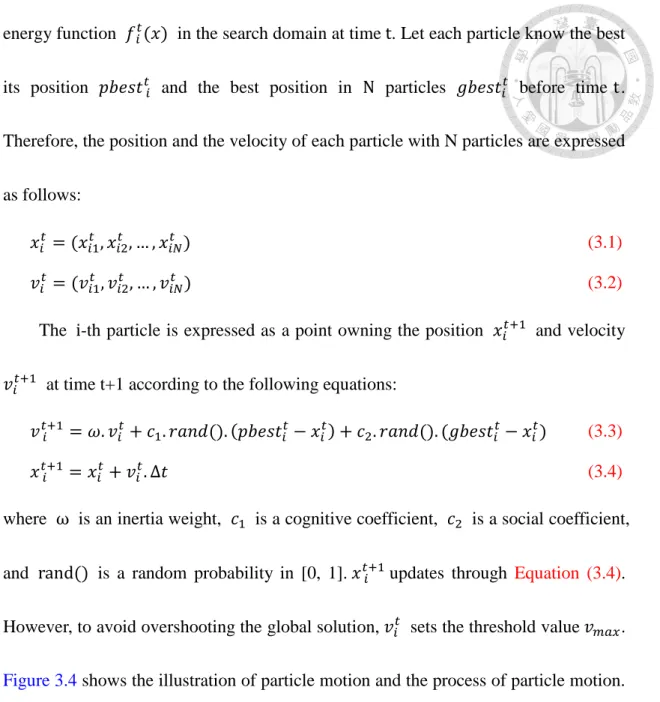
Figure 3.4 shows the illustration of particle motion and the process of particle motion.
In Figure 3.3(a), the plane represents the distance energy function. The curve represents the pass path for each particle by time t. The circle represents current position for each particle. The square presents the best position for each particle. And the triangle represents best position for all particles. Each particle owns its position and velocity. The velocity of each particle is determined by Equation (3.3) and the position of each particle is determined by Equation (3.4). Every particle can affect
19
each other. Figure 3.4(b) shows the flow chart of particle motion. For all particles, the
position and the velocity are set. The energy function is calculated. Then the pbes and the gbes are picked in the particles. And the particles move to next
position. Until the particles stay the same positions, the particles are global optimal positions. If the particles do not stay the same positions, the steps are iterative.
(a)
(b)
Figure 3.3 The Illustration and Process of Particle Selection (a) The illustration of each particle moving
i. The line represents the pass path;
ii. The circle represents current position.
iii. The triangle represents best position in all particles.
iv. And the square is the best position in its particle.
(b) The particle selections of the PSO algorithm
Figure 3.4 shows scan matching points of two data sets results with the LRF. The
scan matching points of two data sets include the red points and the blue points, as
20
shown in Figure 3.4. When the measurement error is not eliminated in time, it causes the inaccurate map. Figure 3.4(a) and (c) show the LRF scan based on odometry in Ming-Da 5F and Ming-Da 4F. Generally, PSO algorithm can reduce the measurement error to enhance the map accuracy, as shown in Figure 3.4 (b) and (d). The other experimental results in scan matching are shown in Section 5.3.
To acquire the more accurate robot position in populated environment, the pedestrian need to be detected. Section 3.3 states dynamic map concept. And Section 4.3 states pedestrian detection based on dynamic map.
21
(a) (b)
(c) (d)
Figure 3.4 Scan Matching 2 Data Result (Target and Source are in the LRF scans) (unit: meter)
(a) Encoder in Ming-Da Building 5F (b) PSO algorithm process from (a) (c) Encoder in Ming-Da Building 4F (d) PSO algorithm process from (c)
3.3 Map Construction
In map construction, occupancy grid map is an important method. Section 3.3.1 uses the occupancy grid map to construct the map. The inverse observation model is used to build static occupancy grid map and dynamic occupancy grid map [22: Wolf &
Sukhatme 2004] in Section 3.3.2.
-8 -6 -4 -2 0 2 4 6
-1 0 1 2 3 4 5 6 7 8 9
-6 -4 -2 0 2 4
-1 0 1 2 3 4 5 6 7 8 9
-8 -6 -4 -2 0 2 4 6 8
-1 0 1 2 3 4 5 6 7 8
-6 -4 -2 0 2 4 6
-2 0 2 4 6 8
22
3.3.1 Grid Map Construction
To make mobile robot move arbitrarily, mapping is a necessary task. However, map construction is difficult for the mobile robot in dynamic environment. What is more, the inaccuracy measurement of LRF scan may cause the map false.
Occupancy grid map is a main method in map construction [23: Thrun et al.
2005]. The occupancy grid map needs a resolution to discretize the environment [55:
Winner et al. 2012]. Therefore, the occupancy grid map can be chosen depending on
the requirements of the precision of the data [55: Winner et al. 2012]. In occupancy grid map, three states include free, occupancy, and unknown. Bayesian probability update robustly applies to the occupancy grid map state as follows:
p 𝑆 |𝑍 , 𝑆 −1 = α. p 𝑆 |𝑍 . p 𝑆 −1|𝑍 −1, 𝑆 −2 (3.5)
Bel 𝑆 = α. p 𝑆 |𝑍 −1 . Bel 𝑆 −1 (3.6)
where the Bayesian probability p 𝑆 |𝑍 , 𝑆 −1 represents Bel 𝑆 . 𝑆 is map state in the specific position at time , and 𝑍 is the measurement in the specific position at time . α is a normalization coefficient.
By Equation (3.6), the occupancy grid map updates the state through iterative method. With this method, the grid occupancy probability only knows the previous occupancy grid map Bel 𝑆 −1 and the inverse observation probability p 𝑆 |𝑍 −1 .
23
3.3.2 Static Map and Dynamic Map
For the occupancy grid map, both the static map concept and the dynamic map concept are proposed [22: Wolf & Sukhatme 2004]. The dynamic map can be estimated from the following equation:
𝐷 |𝑍1, … 𝑍 , 𝑆 −1
1 − 𝐷 |𝑍1, … , 𝑍 , 𝑆 −1 = 𝐷 |𝑍 , 𝑆 −1
1 − 𝐷 |𝑍 , 𝑆 −1 .1 − 𝐷
𝐷 . 𝐷 −1
1 − 𝐷 −1 (3.7) where 𝑆 is the state at time t, 𝑍 is the measurement at time t, and 𝐷 is the
dynamic state at time t.
However, the p 𝐷 |𝑍 , 𝑆 −1 needs the inverse observation model to update.
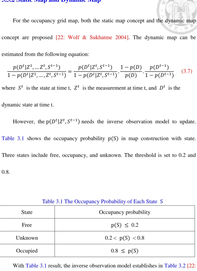
Table 3.1 shows the occupancy probability p S in map construction with state.
Three states include free, occupancy, and unknown. The threshold is set to 0.2 and 0.8.
Table 3.1 The Occupancy Probability of Each State S
State Occupancy probability
Free p S ≤ 0.2
Unknown 0.2 < p S < 0.8
Occupied 0.8 ≤ p S
With Table 3.1 result, the inverse observation model establishes in Table 3.2 [22:
Wolf & Sukhatme 2004]. In [22: Wolf & Sukhatme 2004], Wolf and Sukhatme
propose static map and dynamic map. The static map includes many dynamic
24
obstacles owing to inverse observation model. Since inverse observation model predicts that the state from unknown to occupied is static object, the pedestrian detected with LRF scan by robot may be regarded as static object. The probability is low in dynamic objects. It means that the objects are static. p 𝐷 |𝑍 , 𝑆 −1 is estimated as follows:
Table 3.2 Inverse Observation Model
𝑆 −1 𝑍 p 𝐷 |𝑍 , 𝑆 −1
Free Free Low
Unknown Free Low
Occupied Free Low
Free Occupied High
Unknown Occupied Low
Occupied Occupied Low
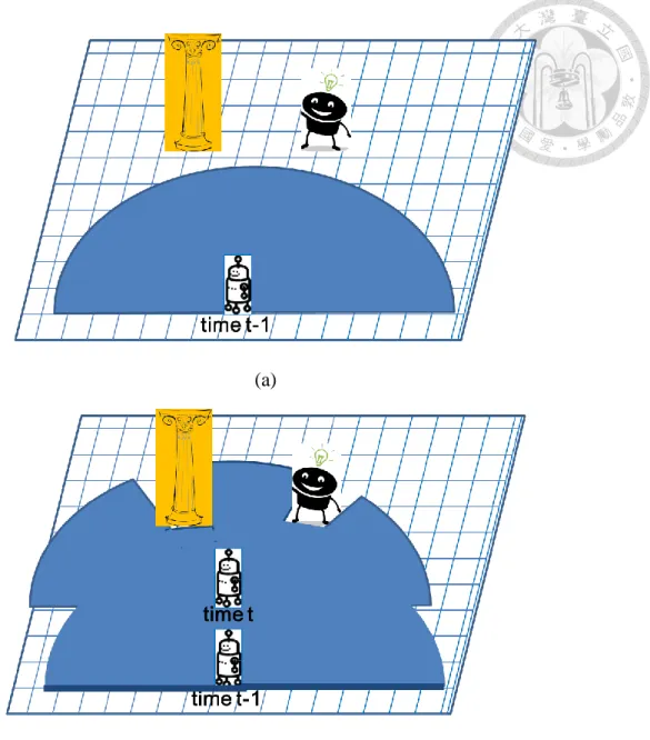
Figure 3.5 demonstrates an example of the inverse observation model analysis of
two consecutive LRF scan. The state of pillar and the state of pedestrian are unknown for the robot at time t-1, while the pillar and the pedestrian are detected for robot at time t. Therefore, the pillar and the pedestrian are regarded as static objects from Table 3.2. In fact, the pillar should be regarded as a static object and the pedestrian
should be regarded as a dynamic object. Table 3.2 is not obviously sufficient. In this scene, the moving object is only pedestrian. The pedestrian detection in Section 4.4 can solve the problem of inverse observation model in Table 3.2.
25
(a)
(b)
Figure 3.5 The Inverse Observation Model Problem (with LRF Scan Grid Map) (a) The pillar and the pedestrian are unknown for the robot at time t-1.
(b) Either the pillar or the pedestrian is regarded as the static in inverse observation model in LRF scan at time t. The pedestrian detection judgment describes in Section 4.3.
26
Chapter 4
Pedestrian Detection and Target Pedestrian Tracking
For pedestrian detection and target pedestrian tracking, both LRF scan and color image are used in this chapter. Section 4.1 states the operation principle of omnidirectional camera and states the problem of the equipment. However, the combination of LRF and omnidirectional camera is difficult since the sensors are not calibrated. The calibration between LRF and omnidirectional camera can be divided into horizontal adjustment, translation, and rotation. In the calibration, the rotation calibration of the combination of LRF and omnidirectional camera is a researchable question. Section 4.2 states rotation calibration of the combination of LRF and omnidirectional camera. For pedestrian detection, the non-pedestrian needs to be filtered out. In this thesis, the methods with the LRF scan and the color image are presented in Section 4.3. LRF scan roughly judges pedestrian. Then the Hough circle transform and the color distribution are the judgment with the color image. With the above methods, the pedestrian detection can be implemented. In target pedestrian tracking, owing to pillars hindering or new pedestrians appearing, the data association
27
may be error between two consecutive LRF scans. The color distribution and the local binary pattern (LBP) algorithm are used in the problems of Section 4.4.
4.1 The Operation Principle of Omnidirectional Camera
In the pedestrian detection problem and the target pedestrian tracking problem of Section 1.2, the LRF scan and the color image should be used. Owing to wide field of
view (FOV), the omnidirectional camera is necessarily used in the problems. Section 4.1.1 states the operation principle of omnidirectional camera. What is more, Section
4.1.2 presents the histogram equalization for low-light omnidirectional camera image.
4.1.1 Introduction of Omnidirectional Camera
The color image is widely used in the mobile robotic field. The color feature plays an important role in pedestrian detection and target pedestrian tracking.
Therefore, the camera is often mounted on the mobile robot.
In this thesis, one of the problems is pillars hindering. The data association may be error between two consecutive LRF scans. To search the target pedestrian, the omnidirectional camera is necessarily used. The omnidirectional camera’s field of view is 360 degree. Therefore, the omnidirectional camera is regarded as an available
28
tool to track the target pedestrian in the pillars hindering problem.
The structure of omnidirectional camera includes a hyperbolic mirror and a camera under the mirror like Figure 4.1 [5: Yagi et al. 2005]. The horizontal passing through the virtual center line (HPVCL) maintains the same height in projection [53:
Yang & Lian 2012], [5: Yagi et al. 2005]. The operation principle makes a light flight
to the upper center 0, c . When the light touches the hyperbolic mirror, the light reflects to the other center 0, −c . The image appears in the process.
Figure 4.1 The Omnidirectional Camera Structure
4.1.2 The Lightness of Omnidirectional Camera
Although the omnidirectional camera owns many advantages, it still overcomes a low-light problem in Figure 4.2. Since the light does not directly flight to image plane,
Camera
29
the color image is dark. The low-light causes the image dark, as shown in Figure 4.3(a). However, the real scene from digital camera is bright, as shown in Figure
4.3(b). That the lighting sources in the beginning put on the floor seems unworkable
because of the unknown environment. The caution leads to two influences. One is the edge threshold value sets small. As a result, the noise easily interfaces the results. The other is each color channel distribution is dense. Therefore, using the color space to tracking target pedestrian is more difficult. Two methods are present to improve the influences. One uses the histogram equalization [6: Gonzalez & Woods 2008] stated in the next paragraph. The other enhances light through the aperture. In this thesis, the histogram equalization is used. With the process, the color image results obtain more robust.
Figure 4.2 The Light Depends on the Active Lighting Source
30
(a) (b)
Figure 4.3 Display Image with Lightness Problem in Ming-Da Building 2F (a) The omnidirectional image has the light problem
(b) The real-scene with digital camera
Histogram Equalization is a method making the intensity in image uniform [6:
Gonzalez & Woods 2008]. The variables are shown in Figure 4.4. Let 𝑃𝑟 𝑟 be the probability of the intensity. Assume the output intensity s, and the definition of s is
the following:
s = T r = ∫ 𝑃𝑟 𝑟 𝑤 𝑑𝑤
0
(4.1)
In this transform, the probability of s is the cumulative distribution function (CDF) of the input 𝑟. And that is proved in [6: Gonzalez & Woods 2008]. The
definition of 𝑃𝑠 is the following:
𝑃𝑠 = { 1 0 ≤ ≤ 1
0 𝑜 ℎ 𝑟𝑤𝑖 (4.2)
where the probability of 𝑃𝑠 is a uniform function. Owing to digital signal, the intensity 𝑘 of image from Equation (4.1) is a discontinuous function in the image
process as follows:
31 𝑘 = ∑ 𝑟 𝑟𝑗
𝑘
𝑗=0
(4.3)
The distribution of intensity is sparse, as shown in Figure 4.3(c), while it is uniform. The edge extraction is more consistent than unprocessed image in dark image. The detail states in Section 5.2.
(a) (b) (c)
Figure 4.4 Each Variable in Histogram Equalization (a) The probability of original intensity: 𝑃𝑟 𝑟
(b) The original intensity transforms output intensity: T r (c) The probability of the output intensity: 𝑃𝑠
4.2 Sensors Calibration
Before using the sensor, the calibration is an important task. In Section 4.2.1, the calibration is divided into horizontal adjustment, translation, and rotation. And the solutions are presented. Section 4.2.2, Section 4.2.3, and Section 4.2.4 are a series of the solutions for the rotation calibration.
32
4.2.1 The Description of Calibration
Combining the LRF and the omnidirectional camera can acquire the abundant information in signal process. Most of all, the data association is the most important problem in sensors calibration. In this calibration, the adjustment of six freedoms is divided into horizontal adjustment, translation, and rotation. The horizontal adjustment uses the gradienter to calibrate the inclination. The translation is to align the geometry center of the LRF and geometry center of the omnidirectional camera in different horizontal plane. The rotation problem is discussed in Section 4.2.2, 4.2.3, and 4.2.4. Figure 4.5 shows the calibration problem for horizontal adjustment, translation, and rotation. The gradienter is used to calibrate the horizontal adjustment.
Furthermore, the vernier caliper is used to align the geometry center. For the rotation problem, the angle matching is a method. In this thesis, the break point and the angular point in LRF scan and vertical line in color image are regarded as feature and presented in Section 4.2.2 and Section 4.2.3.
33
(a) (b)
(c) (d)
Figure 4.5 Calibration Problems: Horizontal Adjustment, Translation, and Rotation (a) The laser range finder and omnidirectional camera
(b) The gradienter for the horizontal adjustment in different plane (c) The vernier for the translation adjustment
(d) The plane rotation problem sketch
4.2.2 Break Point and Angular Point Detection
To do data association, using the feature of data is necessary. The indoor environment is full of the walls. The break point for LRF scan and the angular point for LRF scan are shown in Figure 4.6 [7: Jia et al. 2010]. Here, the break point is presented based on point-distance-based segmentation method [8: Rebai et al. 2009].
The distance between two continuous points in LRF scan is expressed as follows:
𝐷 𝑟, 𝑟 1 = √𝑟 12 + 𝑟 2− 2. 𝑟 12 . 𝑟 2. 𝑐𝑜 ∆𝛼 (4.4) If the distance is more than the threshold value 𝐷 ℎ, the two points are the break
34
points. Therefore the threshold value sets as follows:
𝐷 ℎ = 𝐶0+ 𝐶1. 𝑚𝑖𝑛{𝑟, 𝑟 1} 𝑐𝑜 𝛽 . cos (∆𝛼
2 ) − s n ∆𝛼 2
(4.5)
The parameters 𝐶1, 𝐶0, and β are presented in [8: Rebai et al. 2009]. Next, the
angular point is introduced in [7: Jia et al. 2010]. The start point links end point to be a line. If the distance in point to the line is more than the threshold value δ, the
angular point appears. In Figure 4.6, the idea of feature detection in LRF scan is presented. The ‘V’ presents the break point and the ‘X’ presents the angular point. For the indoor scene, both the break point and the angular point may be corner.
Figure 4.6 The Break Points and Angular Points (With LRF Scan Grid Map) In LRF scan, two consecutive points determinate the corner. Finding the break
point, the angular point owns max distance large a threshold value between two break points link.
35
4.2.3 Vertical Line Detection
The vertical line for color image is also an important feature in unknown indoor environment. The image of omnidirectional camera has distortion. Because of both angular matching and image distortion, the panorama is necessary. To expand the panorama, the projection center search is first of all. To sum up, the process needs to find the projection center, expand the panorama, and detect the vertical line, as shown in Figure 4.13.
The flow chart of projection center search is shown in Figure 4.7. The projection center searching through the HPVCL is set in image center. First, the lower image is
cut. The gray broad in image appears with RGB filter. Then, the region growing and the image filling are used to the image. The data , y, and R relationship is shown as
follows:
− 𝑐1 2+ 𝑦 − 𝑐2 2 = 𝑅2 (4.6)
where the coefficients 𝑐1, and 𝑐2 are unknown. Next, through least square method [10:
Gander et al. 1994], the optimal projection center can be obtained. Finally, the
iterative method is continuous until it converges.
With above method, the optimal projection center converges in the omnidirectional camera image.
36
Figure 4.7 The Flow Chart of Projection Center Search
37
(c)
(a) (d)
(b) (e)
Figure 4.8 Results of the Projection Center Search Algorithm (a) Cut image
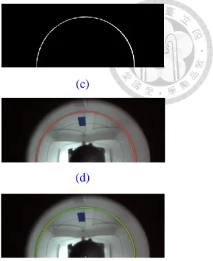
(b) Set the threshold value (c) Region growing (d) Image fill the holes (e) Least square fitting circle
The panorama remedies the distortion image. For [11: Grassi & Okamoto 2006], that the panorama image depends on radius and angle from projection center is shown in Figure 4.9. The vertical axis of panorama is radius and the horizontal axis of panorama is angle. The larger the radius from projection center is, and the less the distortion in omnidirectional image is. The idea of panorama is that the Cartesian coordinate converts the polar coordinate. Figure 4.10 demonstrates an example for panorama image in real scene. Panorama image is shown in Figure 4.10(b).
38
Figure 4.9 The Idea Process of Panorama Image
The vertical axis is radius and the horizontal axis is angle. The larger the radius is, and the less the distortion is.
(a)
(b)
Figure 4.10 Real Scene Image Process in Ming-Da Building 5F (a) Omnidirectional camera image
(b) Panorama image in (a) from the idea of Figure 4.9
39
For the vertical line detection, many edge detectors can be used. For the panorama image, the Sobel vertical edge detection as shown in Figure 4.11 presented in [6: Gonzalez & Woods 2008] seems to be a practical method. Using the Sobel mask in Figure 4.11 does convolution with the original image. If the intensity difference in vertical direction is more than threshold value, the pixel is considered as a vertical edge. The main problem is the lightness of color image stated in Section 4.1.2. If the gradient ∇f is more than threshold T, the vertical edge is detected. However, the threshold value in Sobel vertical edge detection can vary dramatically because of the low-light environment for omnidirectional camera. Figure 4.12 demonstrates an example of low-light environment for omnidirectional camera. The threshold is small, as shown in Figure 4.12(a), the edge can be detected. However, the threshold is large, as shown in Figure 4.12(b). The low-light problem causes the edge threshold often needs to change. Figure 4.14 presents the vertical line extraction results with histogram equalization of low-light environment for omnidirectional camera.
Histogram equalization is used to Figure 4.14(c). The threshold values in Sobel vertical edge detection is set the same. As expected, Figure 4.12(d) appears more vertical line than Figure 4.12(b). Therefore, the vertical line detection includes inputting an image, finding projection center, expanding the panorama, using histogram equalization, using Sobel vertical mask, and using area filtering, as shown
40
in Figure 4.13.
Figure 4.11 The Sobel Vertical Edge Detector
137 I41 115
137 I51 115
137 I61 115
200 I42 55
200 I52 55
200 I62 55
(a) (b)
Figure 4.12 The Example of Two Image for Sobel Vertical Edge Detector (a) The intensity of left column and right column is nearly
(b) The intensity of left column and right column is sparse
Figure 4.13 The Process of Vertical Line Detection
41
(a) (e)
(b) (f)
(c) (g)
(d) (h)
Figure 4.14 Vertical Edge Detector in the Same Threshold Value (a) The original image converts to gray
(b) The edge detector result of (a)
(c) Using histogram equalization process
(d) The edge detector result of (c) and the real scene in digital camera (e) The histogram from (a)
(f) The histogram from (b) (g) The histogram from (c)
(h) The real-scene with digital camera in Ming-Da Building 2F
4.2.4 Data Association
In the sensors calibration, the data association is an important task. However, the distance in LRF scan matches the pixel in color image is a problem. In [13: Bacca et
0 2000 4000 6000 8000 10000 12000
0 50 100 150 200 250
0 2000 4000 6000 8000 10000 12000
0 50 100 150 200 250
0 1000 2000 3000 4000 5000 6000 7000
0 50 100 150 200 250
42
al. 2013], the corner point matches the vertical line like in Figure 4.15(a). What is
more, the dashed plane means the LRF scan plane. In [12: Ueda et al. 2011] and [14:
Scaramuzza et al. 2006], the corner of vertical line is estimated in omnidirectional
image. With the above transform function, the rotation angle can be estimated at the polar coordinates. From vertical line, matching the corner point needs a polynomial function with order 4. In unknown indoor environment, the corner of LRF scan in specific plane and vertical line of color image in digital camera are obvious features.
The results show in Section 5.2.2.
(a) (b)
Figure 4.15 The Data Association Conception Matching the Feature Points
(a) The dashed plane means the LRF scan plane. From vertical line, matching the corner point needs a polynomial function with order 4. The height convert pixel shows in Section 5.2.
(b) A door of Real-Scene for Vertical Line and Corner. In door, the corner of LRF scan in specific plane and vertical line of color image in digital camera are obvious features.
Wall Wall
Corner
Corner Hallway
Vertical Line