服務業之銷售預測、消費者行為及行銷變數之研究

(1)

A Stochastic Model for For ecasting Company Sales for Ser vice Industr ies— An Empir ical Investigation of Life Insur ance Companies

Couchen Wu^* Hsiu-Li Chen^*

*Couchen Wu is an Associate Pr ofessor at Depar tment of Business Administr ation, National Taiwan Institute of Technology

43 Sec. 4 Keelung Road Taipei, Taiwan, R.O.C.

** Hsiu-Li Chen is an Assistant Pr ofessor at Depar tment of Inter national Tr ade, Ming-Chuan Univer sity.

250 sec. 5 Chung Shan N. Road Taipei, Taiwan R.O.C.

Tel: 886-2-8809750 Fax: 886-2-8809751 E-mail: [email protected]

(2)

Abstr act

This paper provides a managerial tool to help marketing managers predict company unit sales as well as identify active customers for any selected period by considering customer use behavior, initial purchase, repeated buying behavior and gamma heterogeneity.

This model is appropriate for many service industries such as life insurance.

(3)

1. Intr oduction

Customer bases are an important foundation of a company’s success. The customer base provides important information for making or examining marketing strategies as well as predicting sales. In general, the broader the customer base the higher the firm’s sales.

An executive who asks customer base questions is implicitly asking questions about

“active” customers, i.e., individuals who have not become disenchanted, taking their business or patronage elsewhere (Schmittlein, et al. 1987). For some industries such as a life insurance company, the customer base exactly represents the company sales or the active customers. Of course, such properties are not unique to life insurance companies. All sorts of organizations exist whose revenues can be counted by customer base, e.g., financial consultant, law consultant, house leasing, machine leasing, telecommunications company (there is a program where you pay a set amount and then enjoy unlimited local calls), cable television service, newspaper subscription, software or machine maintenance, etc.

To predict sales of these businesses for a constant period, some properties concerning customer purchasing behavior should be taken into account. First, instead of counting

(4)

contract time will affect company sales. For example, in a leasing company, its sales depend not only on the leasing units but also on the leasing period which corresponds to the customer contract time. The company’s unit sales would be the sum of each customer’s contract time. If the company has only two leases, one leasing period is four months and the other, five months, then the company's unit sales are nine months. The longer leasing period also provides more opportunities for a company to promote its products or services and new machinery. If the leasing contract holds up longer, in fact, the company has a chance to get more revenue from other services. Second is the regularity of the contract period. Generally, a lease is signed for a period, which may be a week, 2-weeks, a month, a quarter, half year, a year, etc. When the contract is going to expire, the customer can decide whether to renew the contract before or after the expiration date within a given grace period. When a customer renews, he can change the terms of this contract. However, if there are transaction costs, people seldom change contract terms, which would make contract period more regular. Third is learning behavior. A customer, whether they renew the contract or not, is usually impacted significantly by their previous use experience. If the previous service quality meets the expected service quality, or is even better, then they are more likely to renew the contract; otherwise this customer may become disenchanted. Fourth is customer heterogeneity. Customer heterogeneity exists in the contract period as well as in the renewal possibility. Obviously, if the company offers more diversified contract periods for customer selection, the heterogeneity of contract period could be higher. Fifth is customer departure.

Customers can leave by following their account executive to another firm, by moving to another city, etc. As long as the contract ends and is not renewed, it represents customer

(5)

departure, even though they may come back. Finally is the process of capturing new customers. Without capturing new customers in the future, expanding the customer base is futile. Moreover, due to changes in environment and the employment of marketing activities for different period periods, the rate of initial purchase can be distinguished.

The main purpose of this paper is to offer a managerial tool to predict a firm’s unit sales at any time and further to predict company sales for any period. Many relevant variables such as customer use behavior, learning and departure behavior and the initial adoption process are taken into account. All the properties reviewed previously are included and the model is developed for studying the aforementioned industries.

Incorporating customer purchase behavior to predict the firm’s sales has long been of interest to marketing researchers and practitioners. The Negative Binomial Distribution (NBD) model was derived by Ehrenberg in 1959 and gave a good starting point for this research. The so-called NBD-type models assume exponential or Erlang-2 interpurchase time at the individual level. These two distributions with gamma heterogeneity to model aggregate level behavior give an approximate fit for frequently purchased products (Morrison and Schmittlein, 1988). Many researches related to this area are as follows: (i) Extend the so-called negative-binominal-distribution (NBD) model while interpurchase times become more regular (e.g., Chatfield et al 1973, Lawrence 1980, Jeuland et al 1980, Goodharde et al. 1984, Gupta 1988), or the “death rate” is taken into account (Schmittlein et al 1987). (ii) Develop the model by adding explanatory variables to consumer brand choice behavior or capturing the effect of marketing variables on consumers’ purchase

(6)

timing and brand selection models which incorporates the influence of marketing variables, seasonality and trend (e.g., Wagner et al 1986, 1987). (iv) Predict trial and repeat-purchase patterns of new frequently purchased products (e.g., Zufryden 1988). (v) Analyze the order of brand choice process (Bassetal 1984, Kahn et al 1986, Jainet et al 1994). However, there is no research that provides the answer for our questions while incorporating all the aforementioned characteristics.

The objective of our article is therefore to propose a model which incorporates previous studies and complements them by developing a framework to analyze customer buying behavior and forecast company sales, including interpurchase times, learning effect, departure, in-store decision, and unobserved heterogeneity. By allowing for customers’

departure, the other advantage of our model is that it allows us to determine the probability that a customer with a given pattern of purchasing behavior still remains or has departed at any time. Likewise, one of the main focuses is to determine how many purchases are made by a customer at any given period, which is also what the NBD-type models intend to do.

Jeuland, Pass and Wright (1980) extended the NBD-type models. Under the assumption of independence between the Erlang purchasing timing process and zero-order choice process, two processes are compounded: the output of the integrated model includes analytical expressions for market share, the elements of switching matrixes, penetration and duplication. However, it is restricted by the virtual absence of attention to the “departure, learning effect of previous experience and capturing new customers”. Moreover, the purpose of NBD-type papers is for counting the purchases, especially in the steady state, but not for estimating customer base; definitely, this is not designed for evaluating the sales of

(7)

our aforementioned businesses.

One alternative model developed by Schmittlein, Morrison and Colombo (1987) examined consumer purchase patterns by considering “death rates.” In their study, for an individual customer, in addition to the Poisson purchases, the exponential lifetime and gamma heterogeneity for purchasing and death rates, they proved that the model they developed provided the answer for evaluating the customer bases as we intend to do.

However, it is limited by not involving these properties: inducing new customers, regular contract period and learning effect, in evaluating the customer base and sales of the industries as we mentioned previously.

2. The Model

Imagine that you are the marketing manager of an insurance company. You are interested in understanding consumer behavior across population to predict ongoing sales, which would be helpful in planning marketing strategies. To solve these managerial issues, let us start with a brief review of customer contract period.

2.1 Customer contract period

If a customer has different contract terms for each renewal, an irregularity of contract periods would occur; otherwise, the contract periods would be regular. The Erlang distribution is an important generalization of the exponential distribution and can catch the properties of regularities and irregularities well, we therefore model customer contract period as an Erlang distribution (c, u):

(8)

f T c u u T e

c T c

c c uT

( , )

= ^{− −}( ) ≤ ≤ +∞

1

Γ , 0 for integers . (1)

As c=1, equation (1) would be reduced to an exponential density.

2.2 Capturing new customers

Without capturing new customers, it is impossible to extend the customer base. The environment could change or marketing activities can be employed, so the rate of customer’s initial purchase may differ over different periods. While customers’ initial purchasing can not be predicted, it is commonly characterized as a Poisson process (Ross, 1980). However, initial buying rates are not stationary, that is to say, initial purchase rates can be distinct for different periods. Moreover, the duration of each period may vary.

Therefore, in our model, we define λ^{( )}^l as the initial buying rate in period l, l≥1 , and t_lis the end of period l, i.e., t_l₊₁−t_lis the duration of period l. Without loss of generality, we define t₀ =0.

2.2 Repeated buying behavior

Some well-known models such as the NBD assume that the consumer keeps purchasing his or her most preferred brand of product. However, this is not always true.

Repeated buying behavior should be taken into account. Repeated buying probability means the proportion of any brand that is bought on two consecutive purchase occasions. The repeated buying behavior is affected by many factors, such as brand loyalty, promotions,

(9)

price discounts, and last purchase behavior. The last purchase occasion in particular significantly influences the repeated buying probability (Kuehn 1962). The following linear learning model, developed by Bush and Mosteller (1955) is based on this idea.

Linear learning model

The linear model of a customer can be expressed as

R_k =a₀ +a R₁ _k₋₁ +ε_i, 0≤a₁ ≤1, a₀ ≥0, ε_i ~N( ,0 σ²) (2) where：

R i k

a a

k =

=

the repeat buying probability of customer at th renewal automatic renewal probability

the marginal learning propensity.

0

1

Two other learning models: the exponential learning model and the repurchase function of the price model (Lilien, 1974), are also developed based on the concept that the possibility of renewal is impacted significantly by previous experience. In our empirical study, the linear learning model could fit the panel data well.

2.3 Customer departure

A customer who does not renew the contract within the firm’s grace period is treated as a departure. As the probability of the kth renewal is R_k, then the probability of departure at the kth renewal is q_k = −1 R_k. A departure may be permanent or temporary. If the number of returning departures is insignificant, then we would suppose they are involved in

(10)

the new customer stream; otherwise, we should reestimate the initial buying rate for each period. The detailed method will be discussed in section 2.5.2.

2.4 Customer heterogeneity

It is undoubtedly true that customer use behavior and renewal behavior vary according to their personalities, habits, preferences, loyalties and a range of other characteristics. A market may consist of customers who are very heterogeneous, or it may consist of customers who are very similar. One model which is typically applied to model aggregate-level behavior across the whole population is adding gamma heterogeneity to individual renewal rates. In other words, it is assumed that u follows a gamma distribution with parameters γand α over the population of customers, with p.d.f.’s

g u u e

u

( ,

( ) , ,

γ α α

γ α γ

γ γ α

)= ⁻¹ ⁻ > 0 .

Γ (3)

The coefficient of the variation of u is ¹

γ , so the higher the γvalue, the more homogeneous the customers are. In this paper, as we apply the linear learning model to characterize the repeat buying behavior, the heterogeneity of renewal probability would follow the application of the linear learning model, that is ε_iis normally distributed with mean 0 and variance σ².

2.5 Integrated Model

In the present paper, we argue that, despite the return of departed customers, the

(11)

model can be applied by adding the “return” probability. To simplify our discussion, we first study the case those who do not return.

2.5.1. Non-return

Single period

A customer may patronize a business at any time before time t, as noted in the Appendix. The probability that the customer is still active at time t, can be expressed as

p e j t

ck j c t

ck j

c t e

t k

k n

t j

c ck j

j c

ck ck j

= ⋅ − t

− −

− +

− −

=

− − −

=

∑ ∑ ∑

− −

=

R { ( )

( ) !

( )

( ) ! ( ) },

1

1 1

1 1 1

µ µ µ µ

µ (4)

where R_k₋₁ = R R₁⋅ ⋅₂ . . .R_k₋₁ is the probability that he will renew k-1 times, and R_k, 1≤ ≤ −k n 1 is determined by the learning models. Adding the gamma heterogeneity and normalizing the renewal probability to construct an integrated model for the whole population, we obtain ~p_t , the probability of a customer who is active at time t,

~ R { ⁽ ⁾ }

( )!

( )

( )! ( ) ( )

p_t _k e

k

n t

j

c j t ck j

ck j j c

ck c

t ck j ck j

c

t e t r r e

r d

= ^∞ ₋ − −

=

−

=

− − −

− =

− −

− + − −

∫ ∑₀ 1 ∑ ∑

1 1

1 1 1 1

µ µ µ

µ µ α µ αµ

Γ µ

= ∑ ⋅ − ∑ ⋅

− ∑ ⋅ +

= −

=

−

+ − − −+ − −

+ + − −

+ − − −+ − −

= + + − −

− k

n

k j

c j

ck r j ck j

ck r j t

r t

t ck j

c

ck r j ck j

ck r j j c

ck

t

r t

t

ck j c

t r

C

1 1

1

1 1

1

1 1

1

R {

}

( ) ( )

( )

α

α α

α

α α

α

(5)

where R_k−1 is the weighted average probability of repeated buying from all customers.

Let ^Mt be the unit sales at time t. Assuming a customer will only sign one contract at

(12)

newspaper at a time. Thus,^Mt could be regarded as the number of active customers at time t. The initial purchase process is characterized as a Poisson process and the number of active customers is a random partition of the initial purchase process, so ^Mt is a Poisson distribution with mean λ⋅ ⋅t p~ (Wolff 1989),_t

M_t ~ Poisson(λ⋅ ⋅t p~ )_t = 1,2,... . (6)k n Equation (6) could be used by a firm to determine the expectation of current customer use.

Cumulative sales

As discussed previously, for some industries, such as the leasing industry, its total sales in (T T₁, ₂], S T T_t( ₁, ₂) is the integration of the in-constract unit fromT₁ to T₂, that is

S T T M ds

E S T T s pds

T T

s

T T

( , )

( , )) ~ .

1 2

and

(

=

= ⋅ ⋅

∫

^λ

(7)

Multiple periods

Though customer characteristics are more stationary in a stationary period, it is unreasonable to assume the initial purchase retains unchanged. Therefore, we assume initial purchase rates may vary from period to period. If the censor time t is in the second period, i.e., t ∈[ ,t t₁ ₂], we may have two types of customers, those who made their initial purchases in the first period and those who did so in the second period. The probability of a customer who made his initial purchase in the first period and is still active at time t is

(13)

~ { [ ]

[

( ) ( ) ( ) ( ) ( )

p R C

C

t k

j ck r j j c

k n

ck j

ck r j t

t t

r t t

ck j t t

t t t

r t t t t

ck j

c ck r j j c ck

ck j ck r j 1

1 1

1

1 1

1

1 1

= − 1

+

− + − −

=

−

= −+ − −

+ −

− − + − + −

− + −

− −

+ − −

= −+ − −

∑

α

α α α

α α

−_t^t ₊_t ^r ^t₋_t ^{ck j}^{− −} ⁺^{t t}⁻_t _{+ −}_{t t} ^r _{+ −}^{t t}⁻_{t t} ^{ck j}^{− −}

1

1 1

1

1 1

1

(_α^α ) (_α ) (_α^α ) (_α ) ]}

(8)

Otherwise, the probability of a customer making an initial purchase in the second period and still active at time t is

~^{( )} { ( ) ( )

( ) ( )

p R C

C

t k

j ck r j j

c

k n

ck j ck r j

t t

r t t t t

ck j

c ck r j j c ck

ck j ck r j

t t

r t t t t

ck j c

2

1 1

1

1 1

1

1 1

1

= −

− +

− + − −

=

−

= −+ − −

+ −

−

+ − − −

+ − −

= −+ − −

+ −

−

+ − − −

∑

α

α α

α

α α

₍_{t t}₋ ₎₍α_r₋ ₎}

1 1

(9)

According to independent processes of capturing new customers, the number of active customers with initial purchases in the first period and the number of active customers with initial purchases in the second period are independent. The composition of independent Poisson random variables is also a Poisson random variable, we know that the unit sales at time t is a Poisson distribution with mean

E M( _t) =λ^{( )}¹ ⋅ ⋅t₁ p~_t^{( )}¹ +λ^{( )}² ⋅ −(t t₁) ~⋅p_t^{( )}² . (10)

These results could be extended to multiple periods. For t∈(t_l₋₁, ]t_l , l≥2, the probability that the customer is active at time t and his initial purchase is in (t_l₋₁, ] is ~t_l p_t^{( )}^l , where

(14)

~^{( )} { ( ) ( )

( ) ( )

p R C

C tl

k

j c k r j j

c

k n

c kc k rj j

t t

r t t

t t c k j

c c k r j j c

c k

c kc k rj j

t t

r t t

t t

c k j c

l

l l

l

l l

= −

− +

− = + − −

−

= −+ − −

+ −

−

+ − − −

+ − −

= −+ − −

+ −

−

+ − − −

∑

1 1

1

1 1

1

1 1

α

α α

α

α α

α

( )( )}.

t⁻tl r⁻¹

(11)

Otherwise, if a customer's initial purchase is in (t_m₋₁,t_m], where m < l, then the probability that this customer is still active at time t is ~p_t^{( )}^m ,

~p_t^{( )}^m R_k { ^j C ( ( ) ( ) ( ) ( )

ck r j j c

k n

ck j

ck r j t t

tl t t t

r t t t t

ck j t tl

tl t t t

r t t t t

ck

l

l l

l

l l l

l

= ₋ _{+ − −} l

=

−

= −+ − −

− −

− + −

−

+ − − − + −

− + −

−

∑

+ −

∑

¹ 1 ⁻₋ ₋ ⁻₋ ₋ ₋ ⁻₋ 1

1

1 1 1

1 1

1

1 1 1

1 1

α

α α

α

α α − −

+ − −

= −+ − −

− −

− + −

−

+ − − − + −

− + −

−

+ − − −

+

∑

⁻− −

−

− − −

−

j

c ck r j j c

ck

ck j

ck r j t t

tl t t t

r t t t t

ck j t tl

tl t t t

r t t t t

C ^l ck j

l l

l

l l l

l l

1

1 ¹ 1 1

1 1

1

1 1 1

1 1

)

( ⁽ ^{) (} ⁾ ⁽ ^{) (} ⁾ )}.

_α ^α _α _α ^α _α

(12)

Just as in equation (10), we know that the number of in constract units at time t is a Poisson distribution with mean

_E _M _t _t _p _t _t _p

t l

l tl

m

l m

m m tm

( )= ^{( )}( − ₋ )⋅~^{( )} + ⁽ ⁾( − ) ~⁽ ⁾,

=

−

∑ −

λ ₁ λ

1 1

1 (13)

where t0 =0.

Equation (13) allows the marketing manager to predict a company’s unit sales in any selected period as well as across periods.

Cumulative sales

The cumulative unit sales from T₁ to T₂, S T T_t( ₁, ₂), also can be expressed as

S T T M ds

T T

( ,₁ ₂) s .

1

=

∫

2 (14)

(15)

From equations (11), (12), (13) and (14), unit sales are determined by these components:

industry attraction, contract period, initial adoption and the repeat buying probability. Such information is valuable when one is monitoring the size and growth of the customer base or evaluating a product's success based on trial and repeat purchases¹.

Equations (10), (11), and (13) are the main results of this article. These useful properties could help a marketing manager solve some managerial problems.

2.5.2 Returning customers

When the number of returning customers is significant, merely assuming they join the customers’ initial purchasing stream would cause bias in forecasting the sales of the company. However, to realize the real customer behavior for those departures is formidable, since they usually do not notify the firm of the real reason they want to leave. Also, it is hard to predict whether and when a customer wants to return, while, the customer need not answer these questions. Under these situations, we assume there exists a possibility that a departing customer will come back in future periods. Abbreviating the duration of each period, it can be a reasonable assumption, since a customer who renews the contract within the firm’s grace period is regarded as still active. Therefore, when a customer who departs

1 Some useful moments of these distributions are

E( M_t ) = λ ⋅ ⋅t ~p_t =V a r(M _t ).

The variance of M_t is consistent with its mean. Compare this with the NBD model the variance of

(16)

at period l, with probability of returning, r_i^{( )}^l , i=1 2, . . ., in the l+ith period, we suppose he joins the new customer stream of the period l+i.

There is one more concern, that is the assumption that the initial purchase rate is characterized by Poisson. If the returning customers make the process change, the integrated model should be revised entirely. Fortunately, referring to Wolff (1989), the departure process is still a Poisson process. The integration of two independent Poisson processes is still a Poisson process. Therefore, only the process of capturing new customers needs to be revised.

Let λ^{( )}^l , l=1 2, , . . .be the original external initial purchase rate and λ( )l , l=1 2, , ..., be the real initial purchase rate, which involves the returning departures.

Then,

λ( )1 λ λ^{( )}¹ , ( )2 λ^{( )}¹(1 ~ )^{( )}

1 1

= = − p_t r1 (16) and

λ( )l λ(l )( ~p_{t l}⁽^l ⁾)r λ( )( ~j p⁽^j⁾t_j ~p^{( )}t )r , l .

j l

j

j l j

= − − ₋⁻ + − ≥

=

−

+ −

∑

1 1 2

1 1

1 1 2

1 for (17)

The λ( )l depends on λ(l−1 ,… etc., which is computed period by period, so is the) computation of the integrated model. In addition, the integrated model would be performed according to the previous discussion.

3. Panel data application

(17)

The proposed approach is examined with panel data for insurance policies by Aetna Life Insurance Company of America. The dataset covers a panel of 12,741 insurance policies drawn from one Aetna branch for the period 1988-1995. The data contains records of the complete history of each policy in the panel including the insured’s sex, age, premium, policy term, etc. We begin with describing the characteristics of the data set.

From Table 1, those insured with active insurance policies are older than those with inactive insurance policies. They also have higher premiums. Men are more likely to be inactive than women.

Insurance companies allow payment by month, by season, by half-year, or by year.

They also permit payment by cash, credit card or financial transfer. We regard the period between each payment as the “contract period”. Moreover, insurance companies allow change in payment term as well as delay in payment. Therefore, we have a series of random contract periods for each policy. Previous studies show that if the contract period achieves regularity then the Erlang parameter c will become larger (e.g., Chatfield and Goodhardt 1973; Lawrence 1980). In reality, the contract period is more regular than for daily use products.

On the other hand, at the end of each contract period, the policy owner may consider whether to extend the policy or not. If the policy owner doesn’t pay at the end of the contract period, the policy will be invalid and the insured will be permanently cancelled by the insurance company. Thus, we can easily determine whether the insured’s policy is

(18)

cancelled. Otherwise, we regard the probability of extending this policy as the repeat paying probability.

The model is fully determined when the following types of parameters are known: the repeat paying probability, R_k−₁, k ≥1, the order of the Erlang timing process, c, and two parameters which describe the heterogeneity over the population of the renewal rate, a shape parameter, γ , and a scale parameter, α.

In order to determine the repeat paying probability, we employ the essence of Kuehn (1962), that the last use occasion significantly impacts the next contract. The linear learning model is based on consideration of the last use experience. The mean rate R_k can be obtained by the following analytical expression:

R k

k = −1 # of insured who pay less than times and cancel− k total insured insured who pay less than - 1 times .

A “learning effect” exists after the first repurchase, so the OLS procedure can be applied to estimate a₀ and a₁ in the series R_k.

Second, in order to determine the regularity of a payment, the individual distribution of the time intervals between consecutive payments is examined. In the panel data available for this study, when a payment was made, it was recorded; thus, we could directly calculate the mean and standard deviation of individual contract periods. For any random variable, the coefficient of variation (CV) is determined by the ratio of the standard deviation to the mean. The order of Erlang contract period, c, happens to be the inverse of the square of CV

(19)

(i.e., c

= ¹CV2). It is clear that there is some heterogeneity of the population with respect to the order of the contract period process. Thus, Jeuland, et al. (1980) suggested that a first step would be to assume the population is homogeneous with respect to the order and heterogeneous with respect to the second parameter of the Erlang model, which has already been noted as u. Using this idea, each customer’s c is then averaged to yield an overall population c (Gupta 1988). The order of the Erlang process approximates 12 in both periods.

Erlang-12 shows the customer contract periods ( in this case, the check in time) are much more regular than suggested by the exponential distribution.

The finally step is to allow the parameter u to vary for those insured. Many studies have noted that inclusion of heterogeneity improves the model fit (e.g., Gupta 1991). The CV of u is ¹

γ , so γ is the measurement of the heterogeneity across the population of those insured. In this data base, we find that γis 1.3531 and 1.1142 overall and for Pay Life Insurance (PL), respectively. If the average paying rate of one year is 0.1250 overall insurance policies and 0.1176 for PL insurance policies, the other parameters of the gamma distribution αare 0.2160 and 0.1637 overall and for PL, respectively.

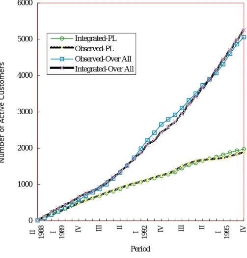
We composed a computer program in C-Language to calculate the probability of customer payments for the integrated model. The predicted results are reported in Table 2 and Figure 1. Active policies of overall policies in 1995 IV were 5060 and the integrated model was predicted to be 5252. An active Policies of PL policies in 1995 IV were 1884 and the integrated model was predicted to be 1969. The predictive quality of the model was

(20)

assessed by using Theil’s U inequality coefficient. U ranges from 0 to 1, where smaller values indicate better predictions. We see from the last column of Table 2, the Theil’s U are 0.0230 for overall insurance policies and 0.0146 for PL insurance policies. The PL case performs well, though its predictions are only marginally better than the overall case.

[Table 1, Table 2, Figure 1]

5. Conclusions

We have attempted to provide a more general framework to analyze company unit sales for some service industries such as life insurance by considering the regularity of contract periods, adding a non-stationary initial purchase rate and including the departure factor. We provided some key extensions which were not investigated simultaneously in previous research. First, because regular purchases exist, we adopt Erlang contract periods in our model. The authors find that customer contract period can be extended to Erlang-c and still be easy to estimate. Second, consideration of customer departure is shown to be necessary when we treat the buying population as having easy exit and entry. In other words, the product may be “dead” in a certain target market segment, and the departure rate of customers should be taken into account. Besides, the assumption of a non-stationary initial purchase rate in different periods makes the prediction closer to the real world.

This model can be used to predict the company’s unit sales or customers retained for a given period or across different periods. Thus, it would be easy to compare customer bases for each package, to specify the value and satisfaction of core customers and measure business performance. According to Aetna insurance company data, the integrated model

(21)

we have developed achieves precise results as can be seen by Theil’s U. This approach also can be applied to leasing industries, financial consultants, cable television services, etc.

Table 1

Insur ed Char acter istics

Insurance Types Insured Characteristics

Average Paying

Rate (one year) Average Age

Average Premium (US $0,000)

Sex (Male)

Over All Active 0.1250 32.16 3.42 47%

Obs=12741 Inactive 0.1231 29.11 3.33 48%

Pay Life Active 0.1173 31.33 2.68 45%

Obs=3133 Inactive 0.1178 28.85 2.65 48%

(22)

Table2

Number of Active Insur ed by Seasonal Per iod

Over All PL Insurance

Period (Seasonal) Observed Frequency

Integrated Model

Observed Frequency

Integrated Model

1988 II 17 30 19 25

III 80 112 87 93

IV 171 245 164 195

1989 I 258 347 243 281

II 348 437 323 355

III 447 532 404 429

IV 574 657 488 517

1990 I 692 755 563 580

II 785 821 633 628

III 875 919 696 686

IV 1002 1062 780 755

1991 I 1163 1192 836 811

II 1331 1352 916 878

III 1522 1525 969 945

IV 1741 1709 1032 1012

1992 I 1989 1891 1073 1063

II 2226 2085 1129 1118

III 2430 2240 1198 1169

IV 2655 2425 1251 1228

1993 I 2793 2578 1307 1278

II 2920 2737 1388 1340

III 3106 2946 1504 1441

IV 3321 3211 1582 1533

1994 I 3505 3421 1649 1588

II 3737 3663 1676 1658

III 3897 3885 1693 1712

IV 4071 4156 1710 1759

1995 I 4314 4444 1734 1820

II 4605 4705 1783 1879

III 4862 4993 1839 1935

IV 5060 5252 1884 1969

Theil’s U 0.0230 0.0146

Note: Predicted number of customers is based on predicted probability of customers.

(23)

Figur e 1 Obser ved Fr equency and Integr ated Model Pr edictions

0 1000 2000 3000 4000 5000 6000

II 1988 I 1989 IV III II I 1992 IV III II I 1995 IV

Period

Number of Active Customers

Integrated-PL Observed-PL Observed-Over All Integrated-Over All