國立臺灣大學電機資訊學院電機工程學系 碩士論文
Department of Electrical Engineering
College of Electrical Engineering and Computer Science
National Taiwan University Master Thesis
新型自由頭部運動之長距離眼動追蹤演算法
Novel Algorithms for Long Distance Free Head Motion Gaze Estimation System
馬政宏 Zheng-Hong Ma
指導教授:陳永耀 博士 Advisor: Yung-Yaw Chen, Ph.D.
中華民國 108 年 01 月
January, 2019
誌謝
在碩士班的兩年半裡,我首先要感謝的就是陳永耀教授。謝謝您在每次會議裡 耐心的指導,不管是做學問的態度或是研究的方法。從您的指導裡,我學到了分析 問題的能力、研究的邏輯、簡報的呈現和表達的能力,這些訓練對於我未來的發展,
實在是相當重要,我也覺得獲益良多。除了學術研究上的指導,您也時常提醒我們 做事的方法及態度,也關心我們研究外的日常生活,讓我在碩士的這段時間裡,感 到充實而且溫馨,非常感謝您的幫助。另外,我也想感謝機械系的顏家鈺教授、醫 學院的何明志教授及醫工所的林文澧教授,謝謝您們在每次會議提供的寶貴意見 和悉心的指導,讓我的研究更臻完善。
感謝實驗室的學長聲仰、一凡,以及其他學弟們的幫助與陪伴,讓我在研究上 更加順利。感謝我的母校,提供我這麼好的資源以及環境,能夠安心且無後顧之憂 的研究與學習。感謝我的家人,給我的支持與鼓勵,讓我能更專心地學習與研究,
你們的陪伴就是我繼續向前的動力。感謝所有幫助過我的人,因為你們熱情無私的 幫助才能有這些成果。
中文摘要
眼動追蹤技術在未來的人機互動以及虛擬實境等領域裡都有很大的應用潛力。
雖然眼對追蹤有長久的研究歷史,時至今日,仍有許多限制。大部分眼動追蹤針對 大約 70 cm 左右的操作距離,並且可能不允許頭部自由運動。對比於靜態坐姿的 追蹤,動態頭部的長距離追蹤則需要更多改善。
本研究旨在開發一定程度頭部運動下的長距離眼動追蹤系統。本研究提出四 種方法且針對其中三種進行實驗。從實驗結果得知,本研究確實有效減少內插式眼 動追蹤法的頭部運動誤差,其中平均誤差均小於 1°,符合精準型的凝視點偵測,
且測試頭部有效運動範圍為 60× 16 × 40以上,操作距離可達 2 米,整體表現相對
於其他研究還算相當不錯。
關鍵字: 遠距離眼動追蹤、內插式眼動追蹤法、頭部運動誤差、瞳孔偵測、映射 函數
ABSTRACT
Gaze estimation is a potential technique in future Human Computer Interaction (HCI) and virtual reality. Although the long history of gaze estimation research, there are still many limits in algorithms nowadays. Oftentimes, many approaches are only valid to use in a distance around 70 cm and might not allow free head motion. This is not desirable when it comes to dynamic and long range head motion gaze estimation instead of stationary sitting gaze estimation.
This work aims at developing long range gaze estimation system which allows certain degree of head motion. And four proposed methods with experiment for three methods are also provided. From the experiment, it could be shown that this work indeed
effectively reduce the head motion error in interpolation based gaze estimation, and the average error are all below 1° which could be regarded as high accuracy gaze estimation.
And the tested effective head motion range could be larger than 60× 16 × 40 and the
operation distance is 2 m. The overall performance of this work is fairly well compared with other researches.
Keywords: Remote eye gaze estimation, Interpolation based gaze estimation, Head
CONTENTS
口試委員會審定書 ...
誌謝 ... i
中文摘要 ... ii
ABSTRACT ... iii
CONTENTS ... iv
LIST OF FIGURES ... viii
LIST OF TABLES ... xvi
Chapter 1 Introduction ... 1
1.1 Motivation and Problem Definition ... 2
1.2 Previous Work of Gaze Estimation System ... 3
1.3 Proposed Approach ... 4
1.4 Thesis Overview ... 5
Chapter 2 Study on Gaze Estimation ... 7
2.1 Eye Structure and Movement type ... 7
2.2 Intrusive Gaze Estimation... 10
2.3 Non-intrusive Gaze Estimation... 11
2.3.1 Interpolation based method ... 12
2.3.2 3D Model Based Method ... 21
2.3.3 Other Methods ... 29
Chapter 3 Fundamentals of 2D Interpolation Based Method ... 32
3.1 Feature Extraction ... 32
3.1.1 Pupil Center Extraction ... 33
3.1.2 Corneal Reflection Extraction ... 35
3.2 Calibration Procedure ... 36
3.3 Mapping Function ... 37
3.3.1 Second order polynomial ... 38
3.3.2 Trigonometric Mapping Function ... 40
3.4 Adaptive Feature Extraction ... 46
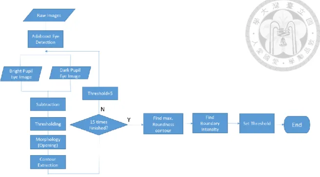
3.4.1 Adaptive Pupil Threshold ... 47
3.4.2 Noise Reduction ... 50
3.4.3 Adaptive Corneal Reflections Threshold ... 52
Chapter 4 Proposed Head Motion Error Compensation Algorithms ... 54
4.1 Geometry Restoration Method ... 55
4.1.1 PCCR transfer relation ... 57
4.1.2 Retrieve Mapping function ... 62
4.1.3 Assessment for Geometry Restoration Method ... 67
4.2.1 Revisit PCCR transfer process ... 71
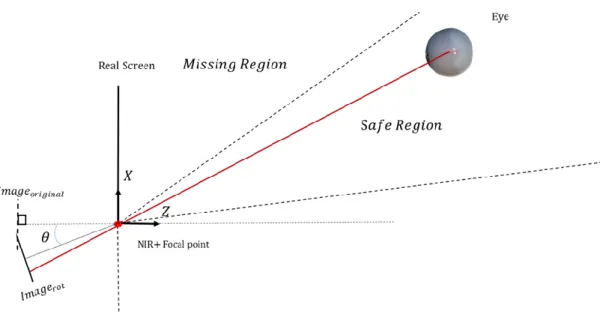
4.2.2 Image Plane Rotation ... 74
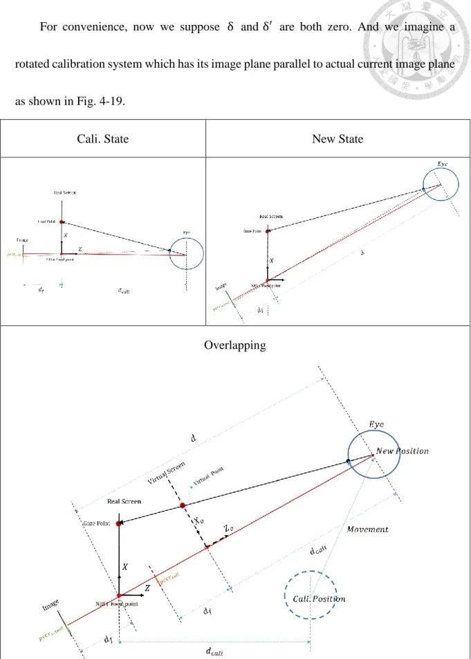
4.2.3 Restore a Rotated Virtual Calibration System ... 76
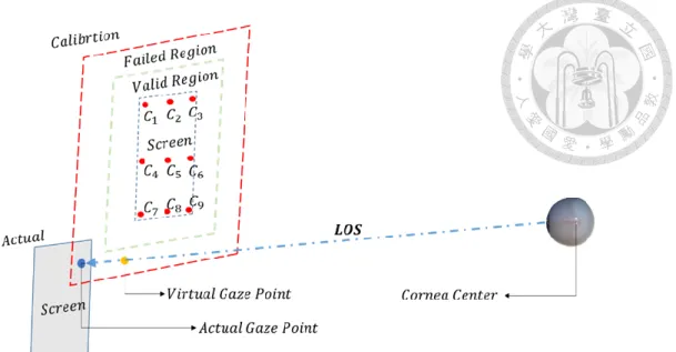
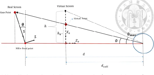
4.2.4 Invalid Mapping Region Examination ... 80
4.2.5 Error Amplification Rate ... 83
4.3 Distance Normalization PCCR method ... 85
4.3.1 PCCR Variation for X-Y Plane Head Motion ... 85
4.3.2 PCCR Variation for Z Direction Head Motion ... 87
4.3.3 Empirical Data Justification ... 88
4.3.4 PCCR Vector with Distance Normalization ... 92
4.3.5 Compensation for General Head Motion ... 95
4.3.6 Assessment for Distance Normalization PCCR Method ... 101
4.4 Area Coordinate Mapping Method ... 102
4.4.1 Area coordinate ... 102
4.4.2 Area Coordinate Defined Feature ... 104
4.4.3 Model Discussion ... 106
4.4.4 Assessment for Area Mapping Method ... 108
Chapter 5 Gaze Estimation Experiment ... 111
5.1 Experiment Setting ... 112
5.2 Calibration Procedure ... 114
5.3 Results of Gaze Estimation ... 118
5.3.1 Area Coordinate Mapping (ACM) Result ... 118
5.3.2 Advanced Geometry Restoration (AGR) Result ... 124
5.3.3 Distance Normalized PCCR (DNP) Result ... 130
5.4 Discussion ... 136
5.5 Comparison ... 138
Chapter 6 Conclusions and Future Work ... 140
REFERENCES ... 142
APPENDIX ... 148
LIST OF FIGURES
Fig. 2-1 Human eye structure [9]... 9
Fig. 2-2 Visual axis in the eye [21]. ... 9
Fig. 2-3 PCCR formation in different head locations [17]. ... 17
Fig. 2-4 PCCR correcting relation in 2D projecting version [17]. ... 18
Fig. 2-5 3D model is reduced into 2D through projection [17]. ... 20
Fig. 2-6 Flow chart of proposed 3D model based method in [33]. ... 22
Fig. 2-7 System configuration with two NIRs and single camera [33]. ... 23
Fig. 2-8 Eye model used to calculate point of gaze [33]. ... 23
Fig. 2-9 Geometry relation to determine cornea center [33]. ... 24
Fig. 2-10 Physical pupil center estimation from the captured image [33]. ... 26
Fig. 2-11 Correcting visual axis deviation via a four points calibration. ... 27
Fig. 2-12 Model and projection used in cross-ratio based method [35]. ... 30
Fig. 2-13 Eye templates used to fit the eye region [38]. ... 31
Fig. 3-1 (a) On-axis light causes bright pupil effect (b) Off-axis light results in dark pupil image (c) bright pupil image (d) dark pupil image ... 34
Fig. 3-2 Pupil contour extraction. ... 34
Fig. 3-3 Corneal reflection extraction flow chart. ... 35
Fig. 3-4 Nine calibration points on screen. ... 37
Fig. 3-5 Calibration points and testing points on the screen. ... 44
Fig. 3-6 General pupil extraction process flow chart. ... 47
Fig. 3-7 Dilemma in setting threshold. ... 48
Fig. 3-8 Minimum rotated bounding rectangular... 49
Fig. 3-9 Flow chart of adapted pupil extraction threshold setting process. ... 50
Fig. 3-10 Magnification subtraction with different multiples. ... 51
Fig. 3-11 Setting optimal multiple process. ... 52
Fig. 3-12 Adapted process for corneal reflection threshold determination. ... 53
Fig. 4-1 PCCR varies with different head positions. [17] ... 55
Fig. 4-2 (a) Head motion effects PCCR in two ways (b) Head motion relative to camera. (c) Head motion relative to screen. ... 56
Fig. 4-3 Fix eye posture and put reference on eye... 58
Fig. 4-4 Diagram for PCCR transfer relation. ... 59
Fig. 4-5 3D is tackled in 2D via projection. ... 60
Fig. 4-6 Projection of pupil center into planes. ... 61
Fig. 4-7 Flow chart of geometry restoration method. ... 63
Fig. 4-8 LOS and actual gaze point determination ... 64
Fig. 4-10 Pupil center to cornea center “r” in human eye. [17] ... 67
Fig. 4-11 Invalid mapping due to virtual point in failed region. ... 69
Fig. 4-12 Intrinsic error amplification. ... 70
Fig. 4-13 Error amplification is proportional to distance. ... 70
Fig. 4-14 Revisit PCCR transfer relation in geometry restoration method ... 72
Fig. 4-15 Observation angle effects PCCR being observed. ... 73
Fig. 4-16 Camera rotates to ensure not missing head when head moves away. ... 74
Fig. 4-17 Calculating 𝑝𝑐𝑐𝑟𝑝𝑎𝑟𝑎𝑙𝑙𝑒𝑙 is needed to exploit parallel plane PCCR transfer process. ... 75
Fig. 4-18 Restoration by rotating calibration state system. ... 77
Fig. 4-19 Restore a rotated calibration state and predict real gaze point. ... 78
Fig. 4-20 (a) Configuration of advanced geometry restoration method for general head motion. And rotated back for clearness as (b). ... 81
Fig. 4-21 Valid mapping condition for d = 𝑑𝑐𝑎𝑙𝑖. ... 82
Fig. 4-22 Utilization rate is used calibrated screen portion ℎ𝑢 over whole screen ℎ. 84 Fig. 4-23 Model illustration for PCCR variation for X-Y plane head motion. ... 86
Fig. 4-24 Model illustration for PCCR variation in Z direction head motion. ... 87
Fig. 4-25 Error for X direction head movement. ... 89
Fig. 4-26 Error for Z direction head movement. ... 89
Fig. 4-27 Absolute values for PCCR in different Z positions. ... 91
Fig. 4-28 Estimation for 𝑝𝑐𝑐𝑟𝑏𝑖𝑎𝑠 due to deviation in optical axis and visual axis. . 92
Fig. 4-29 Experiment setting for testing the correct power for normalized PCCR relation. ... 93
Fig. 4-30 Using Calibration in C8 for 𝑝𝑐𝑐𝑟𝑏𝑖𝑎𝑠 estimation ... 95
Fig. 4-31 Camera equipped on pan tilt unit. ... 96
Fig. 4-32 Focal point of camera is collimated with cornea center via rotation. ... 96
Fig. 4-33 Flow chart of distance normalization method. ... 97
Fig. 4-34 Head position is described by polar coordinate. ... 98
Fig. 4-35 Illustration of distance normalization method. ... 98
Fig. 4-36 3D illustration for Distance Normalization PCCR method. ... 99
Fig. 4-37 Coordinate rotation from 𝑛1 𝑡𝑜 𝑛2. ... 99
Fig. 4-38 Relation for head position and pan tilt angles. ... 100
Fig. 4-39 Position described by (a) Cartesian coordinate (b) Area coordinate. ... 103
Fig. 4-40 (a) System configuration for area coordinate mapping method. (b) Three corneal reflections serves as reference points. ... 105
Fig. 4-41 Position of pupil center is defined by area coordinate using ∆𝐴𝐵𝐶. ... 105
Fig. 4-42 Patterns are similar after projection among three planes. ... 107
similar. ... 108
Fig. 5-1 System setting overview. ... 112
Fig. 5-2 System configuration. ... 113
Fig. 5-3 Experiment setting. ... 113
Fig. 5-4 (a) Camera position calibration. (b) Screen position calibration. ... 114
Fig. 5-5 Focal point estimation. ... 115
Fig. 5-6 Calibration and testing points on the screen. ... 116
Fig. 5-7 Regression error for area coordinate mapping. ... 117
Fig. 5-8 Regression error for PCCR mapping. ... 117
Fig. 5-9 Degree error for ACM in different position and error reduced rate relative to traditional PCCR method. ... 123
Fig. 5-10 Degree error for AGR in different position and error reduced rate relative to traditional PCCR method. ... 129
Fig. 5-11 Degree error for DNP in different position and error reduced rate relative to traditional PCCR method. Where solid circle positions use (4-32) and empty circle positions use (4-34). ... 135
Fig. A-1 Ideal “+” and estimated “o” gaze points for ACM in position 1. ... 148
Fig. A-2 Ideal “+” and estimated “o” gaze points for ACM in position 2. ... 149
Fig. A-3 Ideal “+” and estimated “o” gaze points for ACM in position 3. ... 150
Fig. A-4 Ideal “+” and estimated “o” gaze points for ACM in position 4. ... 151
Fig. A-5 Ideal “+” and estimated “o” gaze points for ACM in position 5. ... 152
Fig. A-6 Ideal “+” and estimated “o” gaze points for ACM in position 6. ... 153
Fig. A-7 Ideal “+” and estimated “o” gaze points for ACM in position 7. ... 154
Fig. A-8 Ideal “+” and estimated “o” gaze points for ACM in position 8. ... 155
Fig. A-9 Ideal “+” and estimated “o” gaze points for ACM in position 9. ... 156
Fig. A-10 Ideal “+” and estimated “o” gaze points for ACM in position 10. ... 157
Fig. A-11 Ideal “+” and estimated “o” gaze points for ACM in position 11. ... 158
Fig. A-12 Ideal “+” and estimated “o” gaze points for ACM in position 12. ... 159
Fig. A-13 Ideal “+” and estimated “o” gaze points for AGR in position 1. ... 160
Fig. A-14 Ideal “+” and estimated “o” gaze points for AGR in position 2. ... 161
Fig. A-15 Ideal “+” and estimated “o” gaze points w/o AGR in position 2. ... 162
Fig. A-16 Ideal “+” and estimated “o” gaze points for AGR in position 3. ... 163
Fig. A-17 Ideal “+” and estimated “o” gaze points w/o AGR in position 3. ... 163
Fig. A-18 Ideal “+” and estimated “o” gaze points for AGR in position 4. ... 164
Fig. A-19 Ideal “+” and estimated “o” gaze points w/o AGR in position 4. ... 165
Fig. A-20 Ideal “+” and estimated “o” gaze points for AGR in position 5. ... 166
Fig. A-21 Ideal “+” and estimated “o” gaze points w/o AGR in position 5. ... 166
Fig. A-23 Ideal “+” and estimated “o” gaze points w/o AGR in position 6. ... 168
Fig. A-24 Ideal “+” and estimated “o” gaze points for AGR in position 7. ... 169
Fig. A-25 Ideal “+” and estimated “o” gaze points w/o AGR in position 7. ... 169
Fig. A-26 Ideal “+” and estimated “o” gaze points for AGR in position 8. ... 170
Fig. A-27 Ideal “+” and estimated “o” gaze points w/o AGR in position 8. ... 171
Fig. A-28 Ideal “+” and estimated “o” gaze points for AGR in position 9. ... 172
Fig. A-29 Ideal “+” and estimated “o” gaze points w/o AGR in position 9. ... 172
Fig. A-30 Ideal “+” and estimated “o” gaze points for AGR in position 10. ... 173
Fig. A-31 Ideal “+” and estimated “o” gaze points w/o AGR in position 10. ... 174
Fig. A-32 Ideal “+” and estimated “o” gaze points for AGR in position 11. ... 175
Fig. A-33 Ideal “+” and estimated “o” gaze points w/o AGR in position 11. ... 175
Fig. A-34 Ideal “+” and estimated “o” gaze points for AGR in position 12. ... 176
Fig. A-35 Ideal “+” and estimated “o” gaze points w/o AGR in position 12. ... 177
Fig. A-36 Ideal “+” and estimated “o” gaze points for DNP in position 1. ... 178
Fig. A-37 Ideal “+” and estimated “o” gaze points for DNP (4-34) in position 2. ... 179
Fig. A-38 Ideal “+” and estimated “o” gaze points for DNP (4-32) in position 2. ... 179
Fig. A-39 Ideal “+” and estimated “o” gaze points for DNP (4-34) in position 3. ... 180
Fig. A-40 Ideal “+” and estimated “o” gaze points for DNP (4-32) in position 3. ... 181
Fig. A-41 Ideal “+” and estimated “o” gaze points for DNP (4-34) in position 4. ... 182
Fig. A-42 Ideal “+” and estimated “o” gaze points for DNP (4-32) in position 4. ... 182
Fig. A-43 Ideal “+” and estimated “o” gaze points for DNP (4-34) in position 5. ... 183
Fig. A-44 Ideal “+” and estimated “o” gaze points for DNP (4-32) in position 5. ... 184
Fig. A-45 Ideal “+” and estimated “o” gaze points for DNP (4-34) in position 6. ... 185
Fig. A-46 Ideal “+” and estimated “o” gaze points for DNP (4-32) in position 6. ... 185
Fig. A-47 Ideal “+” and estimated “o” gaze points for DNP (4-34) in position 7. ... 186
Fig. A-48 Ideal “+” and estimated “o” gaze points for DNP (4-32) in position 7. ... 187
Fig. A-49 Ideal “+” and estimated “o” gaze points for DNP (4-34) in position 8. ... 188
Fig. A-50 Ideal “+” and estimated “o” gaze points for DNP (4-32) in position 8. ... 188
Fig. A-51 Ideal “+” and estimated “o” gaze points for DNP (4-34) in position 9. ... 189
Fig. A-52 Ideal “+” and estimated “o” gaze points for DNP (4-32) in position 9. ... 190
Fig. A-53 Ideal “+” and estimated “o” gaze points for DNP (4-34) in position 10. ... 191
Fig. A-54 Ideal “+” and estimated “o” gaze points for DNP (4-32) in position 10. ... 191
Fig. A-55 Ideal “+” and estimated “o” gaze points for DNP (4-34) in position 11. ... 192
Fig. A-56 Ideal “+” and estimated “o” gaze points for DNP (4-32) in position 11. ... 193
Fig. A-57 Ideal “+” and estimated “o” gaze points for DNP (4-34) in position 12. ... 194
Fig. A-58 Ideal “+” and estimated “o” gaze points for DNP (4-32) in position 12. ... 194
LIST OF TABLES
Table 2-1 Types of eye movements [22]. ... 10
Table 3-1 17 Independent trigonometric candidate terms ... 40
Table 3-2 Process of 17 terms elimination and reservation. ... 43
Table 3-3 Trigonometric mapping function fitting and testing error. ... 44
Table 4-1 PCCRs in Different Distance to Screen. ... 90
Table 4-2 Result for testing different power for normalized PCCR relation. ... 94
Table 5-1 System specification. ... 111
Table 5-2 Coordinates of calibration points. ... 116
Table 5-3 Comparison for with and without ACM in position 1. ... 119
Table 5-4 Comparison for with and without ACM in position 2. ... 119
Table 5-5 Comparison for with and without ACM in position 3. ... 119
Table 5-6 Comparison for with and without ACM in position 4. ... 120
Table 5-7 Comparison for with and without ACM in position 5. ... 120
Table 5-8 Comparison for with and without ACM in position 6. ... 120
Table 5-9 Comparison for with and without ACM in position 7. ... 121
Table 5-10 Comparison for with and without ACM in position 8. ... 121
Table 5-11 Comparison for with and without ACM in position 9. ... 121
Table 5-12 Comparison for with and without ACM in position 10. ... 122
Table 5-13 Comparison for with and without ACM in position 11. ... 122
Table 5-14 Comparison for with and without ACM in position 12. ... 122
Table 5-15 Overall performance for ACM in different head positions. ... 123
Table 5-16 AGR in position 1. ... 124
Table 5-17 Comparison for with and without AGR in position 2. ... 125
Table 5-18 Comparison for with and without AGR in position 3. ... 125
Table 5-19 Comparison for with and without AGR in position 4. ... 125
Table 5-20 Comparison for with and without AGR in position 5. ... 126
Table 5-21 Comparison for with and without AGR in position 6. ... 126
Table 5-22 Comparison for with and without AGR in position 7. ... 126
Table 5-23 Comparison for with and without AGR in position 8. ... 127
Table 5-24 Comparison for with and without AGR in position 9. ... 127
Table 5-25 Comparison for with and without AGR in position 10. ... 127
Table 5-26 Comparison for with and without AGR in position 11. ... 128
Table 5-27 Comparison for with and without AGR in position 12. ... 128
Table 5-28 Overall performance for AGR in different head positions for Fig. 5-10. . 129
Table 5-29 DNP in position 1. ... 130
Table 5-31 Comparison for with and without DNP in position 3. ... 131
Table 5-32 Comparison for with and without DNP in position 4. ... 131
Table 5-33 Comparison for with and without DNP in position 5. ... 132
Table 5-34 Comparison for with and without DNP in position 6. ... 132
Table 5-35 Comparison for with and without DNP in position 7. ... 132
Table 5-36 Comparison for with and without DNP in position 8. ... 133
Table 5-37 Comparison for with and without DNP in position 9. ... 133
Table 5-38 Comparison for with and without DNP in position 10. ... 133
Table 5-39 Comparison for with and without DNP in position 11. ... 134
Table 5-40 Comparison for with and without DNP in position 12. ... 134
Table 5-41 Overall performance for DNP in different head positions of Fig. 5-11. ... 135
Table 5-42 Accuracy performances of proposed methods. ... 138
Table 5-43 Accuracy performances of others’ works [17]. ... 139
Table 5-44 More accuracy performances of others’ works [15]. ... 139
Table A-1 ACM result for 16 testing points in position 1. ... 148
Table A-2 ACM result for 16 testing points in position 2. ... 149
Table A-3 ACM result for 16 testing points in position 3. ... 150
Table A-4 ACM result for 16 testing points in position 4. ... 151
Table A-5 ACM result for 16 testing points in position 5. ... 152
Table A-6 ACM result for 16 testing points in position 6. ... 153
Table A-7 ACM result for 16 testing points in position 7. ... 154
Table A-8 ACM result for 16 testing points in position 8. ... 155
Table A-9 ACM result for 16 testing points in position 9. ... 156
Table A-10 ACM result for 16 testing points in position 10. ... 157
Table A-11 ACM result for 16 testing points in position 11. ... 158
Table A-12 ACM result for 16 testing points in position 12. ... 159
Table A-13 AGR result for 16 testing points in position 1. ... 160
Table A-14 AGR result for 16 testing points in position 2. ... 161
Table A-15 AGR result for 16 testing points in position 3. ... 162
Table A-16 AGR result for 16 testing points in position 4. ... 164
Table A-17 AGR result for 16 testing points in position 5. ... 165
Table A-18 AGR result for 16 testing points in position 6. ... 167
Table A-19 AGR result for 16 testing points in position 7. ... 168
Table A-20 AGR result for 16 testing points in position 8. ... 170
Table A-21 AGR result for 16 testing points in position 9. ... 171
Table A-22 AGR result for 16 testing points in position 10. ... 173
Table A-23 AGR result for 16 testing points in position 11. ... 174
Table A-25 DNP result for 16 testing points in position 1. ... 177
Table A-26 DNP (4-34) result for 16 testing points in position 2. ... 178
Table A-27 DNP (4-32) result for 16 testing points in position 3. ... 180
Table A-28 DNP (4-32) result for 16 testing points in position 4. ... 181
Table A-29 DNP (4-34) result for 16 testing points in position 5. ... 183
Table A-30 DNP (4-32) result for 16 testing points in position 6. ... 184
Table A-31 DNP (4-32) result for 16 testing points in position 7. ... 186
Table A-32 DNP (4-34) result for 16 testing points in position 8. ... 187
Table A-33 DNP (4-32) result for 16 testing points in position 9. ... 189
Table A-34 DNP (4-32) result for 16 testing points in position 10. ... 190
Table A-35 DNP (4-34) result for 16 testing points in position 11. ... 192
Table A-36 DNP (4-32) result for 16 testing points in position 12. ... 193
Chapter 1 Introduction
Gaze estimation serves as a mighty tool in many fields of applications such as human computer interaction (HCI), psychology, human behaviors research, and marketing analysis [1], [2]. By simply telling where a subject is looking at, we can infer one’s intention and psychological activities for research purpose. Besides, subject is also able to convey their intention or command through their visual attention, and this presents a platform for communication between human and machine. Gaze estimation technique has been studied over two decades, and thus many methods has been proposed. Generally, there can be divided into five categories in terms of non-intrusive method. Each category is based on completely distinct strategy and to some degree is platform dependent. For example, 2D regression based method and 3D model based method often use high resolution cameras equipped with lens to gain clear image in eye, others might merely need low resolution face image and then use it to get results. In this essay, our method is essentially based on traditional 2D PCCR regression based method, which is proper for long range gaze manipulation environment. 2D PCCR regression based method has those desirable attributes, such as high accuracy, simplicity, moderate calibration effort, easiness of implementation and so on. However, 2D PCCR methods also possess a serious
Therefore, it has always been highly concerned how to compensate for head moving error.
When it comes to coping with head moving error, one might argue why not just adopt another method based on different estimation strategy that accommodates head movement in the first place. Undoubtedly, fixing such error in purely regression based method is somewhat against its nature. Nevertheless, despite all these challenges, we still assume that 2D regression based method has its excellent characteristics that are so far hardly replaced by other methods and thus worth taken. As a result, what we attempt to do is reserving original PCCR method but focusing on how we can reduce or restore all those error at least to calibration scenario. The idea behind is we consider the 3D geometry and try to find a transformation between calibration state and actual state thus finally restore all those dependent factors to the equivalent calibration state and then we can hold our mapping function correct without additional user effort. Or use head motion invariance feature as input feature in interpolation based method.
1.1 Motivation and Problem Definition
Gaze estimation is a valuable technique since it gives an intuitive way for human computer interactions. However, to estimate human gaze from facial image is not an easy work and worth more research to develop a more robust estimation. Many
commercial products reports a limited using range especially target distance and often yield accuracy that ranges from 0.5°- 1°. Nevertheless, general commercial gaze
estimation products are often still expensive [18] which might not be easily affordable.
This work aims at realizing a long range gaze estimation system which allows larger free head motion range. However, this is somehow a dilemma since long range gaze estimation often requires using interpolation based gaze estimation. But interpolation based methods are found on calibration data which results in small head motion range in traditional interpolation or to say calibration based method. This work thus is set to be based on interpolation based gaze estimation method and proposes several head motion error compensation algorithms.
1.2 Previous Work of Gaze Estimation System
There are lots of work done in gaze estimation techniques. And the development of approaches are influenced by other more general and basic research fields such as artificial intelligence and also the overall enhancement of related hardware. Generally, in addition to accuracy performance, system nowadays prefers low intrusiveness, easy implementation, low calibration effort, low cost system and robustness in different
so on. Oftentimes, the complexity and method adopted depends on the applications.
Different application implemented on different platform such as webcam and mobile device or long focus camera with large screen. And also, generally, algorithm complexity increased dramatically when more and more accurate result is needed which is also dependent on the application scenario. In conclusion, interpolation based and 3D geometric based gazed estimation are quite well-developed remote gaze estimation methods and possess high accuracy. Other methods such as appearance based method, shaped based method and cross-ratio based method might have either less works or lower accuracy which might emphasize on easy implementation, low calibration effort and low cost systems.
1.3 Proposed Approach
As prior discussion, this work aims at long distance (2m) gaze estimation and among all the works of remote eye gaze estimation, the only method which has high accuracy and long distance robustness is interpolation base gaze estimation method. However, this method has a well-known shortcoming that the accuracy fails when the head moves away from calibration position. Therefore, this work focuses on reducing the increased head motion error in traditional interpolation based method and provides four different
approaches with various benefits. First three methods rely on geometry model and head position to construct a transfer relation for actual PCCR vector and its corresponding calibration state vector. By the geometry restoration process, the compensated real gaze point could be inferred back. The differences among these three methods are model assumption and the restored geometry. Different model has different pros and cons. Since it relies on real space geometry, it is no wonder that these three methods must be given
the current head or cornea center position and this requires some additional equipment and estimation process to measure the current user’s head position in real time. And it
might be considered as an additional burden to implement these known head position error compensation algorithms. Thus, this work presented the last method which does not need to provide any additional information including head position. All the works in this method are fairly the same as traditional interpolation based method, the only difference is the mapping feature is replaced by pupil position measured in area coordinates. And might possibly have a more robust free head motion accuracy relative to traditional PCCR interpolation based method.
1.4 Thesis Overview
including eye structure and gaze estimation algorithms. Second, the foundation of interpolation based method including feature extraction, calibration and mapping function are discussed in detail as Chapter 3. Third, the major proposed works of four different algorithms dealing with head motion error in traditional interpolation based method are presented in Chapter 4. Fourth, the experiment setting with system calibration and result are shown in Chapter 5. Finally, conclusion and future work are provided in Chapter 6.
Chapter 2 Study on Gaze Estimation
Vision could be considered the most important way of perception to outer world for human beings and it is highly evolved with a large portion of human brain responsible for processing and analyzing sense input from sight. Nowadays, many researchers are getting more and more interested in gaze estimation techniques since gaze is not only a input sense to human, but also reveals much important information such as human intention, attention, cognitive or mental states and so on [1]. Various field concerns different types of eye behaviors such as eye disease diagnosis in medical field, cognitive process in psychological field [4], [5] and human behavior researches in marketing. Among all the extensions of gaze estimation technique, the most prospective and popular application is human computer interaction (HCI) [6]-[8].
2.1 Eye Structure and Movement type
Before talking about how gaze estimation technique is done, it is appropriate to first introduce basic knowledge of eye structure and eye movement type.
First, eye is roughly spherical with a radius about 12-13 mm. Outer appearance of eye are pupil, iris and sclera. Iris is a colored big circle in the eye. Sclera is the large outer white part. Pupil is located in the center of iris and responsible for controlling the amount of the entering light and would expand and contract due to different environmental illumination condition. Cornea is a surface transparent membrane protecting the bottom part of the eye with a radius about 7.8mm [20].
Behind the iris, a biconvex multilayered structure is called crystalline lens which would vary its shape to form the image on the retina. Retina is a layer coated with lots of photosensitive cells locating at the back of the eye. Fovea is a small spot which is the finest part of retina and has a lot of color sensitive cells and bonding to many optic nerve relative to peripheral region of retina. When human gazes at something, image of that thing is located at this spot. The line connecting fovea and cornea center is called visual axis or Line of Sight (LOS). And when it comes to gaze estimation, the other line which is prone to mistake as LOS is optical axis or to say Line of Gaze (LOG), which is the central axis of eye going through pupil center and cornea center. The visual axis and optical axis intersect at cornea center which is a nodal point of the eye [18]. These two important lines related to gaze estimation reports individual dependent angular offset. Typical adult show a horizontally 4-5 degrees and vertically 1.5 degrees deviation between those two axes and might have
up to 3 degrees variations between subjects [19].
Fig. 2-1 Human eye structure [9].
Fig. 2-2 Visual axis in the eye [21].
The basic classification of eye movement could be classified as fixations and saccades. Fixation occurs when the visual attention stays at a specific small region for at least 80-100ms [18]. It is important since it happens when a subject is focused or attentive to something. It is most studied in psychology, neuroscience and so on. Saccadic eye movement happens between two fixations which brings the interested object into vision center. Further classification of eye movement is shown in Table 2-1.
Table 2-1 Types of eye movements [22].
2.2 Intrusive Gaze Estimation
Intrusive gaze estimation methods appear a few decades earlier than non-intrusive
methods which requires physical contact with the users. In 1905, Judd, McAllister, and
Steele placed a reflective white dot on the eye to measure the gaze direction [24]. A Psychologist attached a tiny mirror with suction cup to the eye to detect the subject’s gaze
[23]. And some attached a number of electrodes around the eye which allowed to register the eyeball movement by measuring skin potential difference [25], [26]. Or some might put coil in contact lens and measured the voltage to estimate gaze [27].
2.3 Non-intrusive Gaze Estimation
In comparison to intrusive gaze estimation method, recent work on gaze estimation often emphasizes estimation without intrusive process, in other words, non-intrusive gaze estimation is required. This goal is fulfilled in the help of current high resolution digital cameras and high quality computers. Non-intrusive gaze estimation is usually based on face image captured by camera and thus also known as video based methods. Video based method is now a mainstream gaze estimation method nowadays thanks to its accuracy, convenience and, most important, much more comfortable user experience. Video based method could be divided into five categories, interpolation based method, 3D model based method, appearance based method, cross-ratio based method and shape based
are widely used in many high-end commercial gaze estimation products.
2.3.1 Interpolation based method
Interpolation based method could be regarded as one of the earliest approach in video based gaze estimation. As early as 1974, Merchant [10] used an IR light source which generates corneal reflection, and exploit vector formed by corneal reflection and pupil center to define an eye movement feature, which is known as PCCR vector. If all variables are fixed and only eye rotates to change gaze point or line of sight, then specific PCCR represents and therefore would only map to a unique gaze point on the screen coordinate.
Basic principle is then developed, interpolation based method first collects a few known calibration ground truth points with their corresponding PCCR vectors and uses these data to do a regression process, which involves a fitting math model with some unknown variables and use the calibration data to determine these unknowns in the model function that gives the optimal approximation to all those calibration ground truth data. The question follows is how to acquire an effective model. This could be the key and the hardest part of whether this approach would success or not. It is almost no doubt that realistic gaze estimation model might turn out to be really complex and the mapping model must coincide with some of the intrinsic behavior between PCCR vector and gaze
point on the screen. An exact mapping relation based on theoretical system model could be hard and lack of closed form. Nevertheless, it is intuitive to realize that rough behavior of PCCR is consistent and predictable when a subjective changes gaze point on the screen.
It is to say, the question now is how accurate the gaze estimation system should attain.
Fine and highly precise gaze estimation could be far more difficult than a rough or middle accurate gaze estimation system. Fortunately, it is proven by others’ work [11], [12], [14]
that merely a simple second order polynomial could fulfill an effective and efficient mapping with tolerable calibration effort. Form of mapping function directly influences how many calibration points should be done. Generally, more calibration points and more complex the mapping model adopted, more accurate the result is supposed to be. However, calibration process must be regarded as an important drawback in gaze estimation system since if calibration is done everywhere on the screen, then no wonder one could tell the exact gaze point without a second thought. And among all the other non-intrusive gaze estimation methods, it is no doubt that the worst thing of interpolation based approaches is that much more calibration effort done must be involved in this method compared to other methods. To sum up, interpolation based method could also be considered as calibration based method since the actual principle behind is found on calibration process and all the calibration points must be used efficiently since too much calibration effort is
The most common and classic feature used in traditional interpolation based method is PCCR vector which is formed be pupil center and corneal reflection and could also be called as PCCR method. PCCR method usually requires high resolution eye image since PCCR feature is fairly small. And it could be easily shown in experiment that how decrease resolution of eye image could undermine the estimation accuracy due to quantization error. Practical implementation of interpolation based method could be divided into two major parts. The first part is feature detection which involves extracting pupil center and corneal reflection. This part relies on techniques in image processing if system needs to be implemented in real time and automatically. This part directly effects estimation accuracy and must be processed as quickly as possible in real time implementation. Image processing often requires lots of computation effort and consequently takes much time. However, many gaze estimation systems rely on a special identity of pupil known as bright pupil effect to enhance the accuracy and speed of pupil extraction [13]. This part would be introduced in later chapter. The other part is gaze estimation algorithm. Traditional PCCR method presumes that PCCR would map to a unique point since corneal reflection is assumed to be a stationary reference point while head position is fixed. However, this assumption would no longer hold when head starts to move and mapping function would fail in yielding accurate gaze point [14], [15]. In other words, interpolation based method constructs mapping relation for PCCR and gaze
point on screen via calibration and not stepping into the interactions of all the related parameters. It is an intrinsic weakness of calibration based method without model analysis that the actual mechanism is not conceivable and all we could do when the operation condition changes is repeating the calibration process and thus gain the novel input output mapping relation which is obviously neither flexible nor robust. Despite all these downsides of interpolation based method, there are still some good attributes of this method that make this approach still popular in some applications and commercial products. First, this method reduces all other kinds of complicated calibration such as camera calibration, geometric calibration and personal calibration to only one gaze mapping calibration and therefore it is much easier in terms of implementation. Second, when head position is fixed, it could easily yield a stable and accurate performance result since high resolution image and strongly correlated feature are adopted in this method.
Third, also as a result of its stableness, small detection or measurement error would not seriously amplify the final estimation error and consequently this method is much suitable and reliable in long distance remote gaze estimation which is not the case in ordinary scenario sitting in front of the monitor with distance ranges from 50 to 70 cm. Due to all the above advantages, calibration based method is still valuable to preserve and worth some effort to compensate for the original head motion error and also this issue often
introduce some related works done in handling head motion error in interpolation based
method.
Zhiwei Zhu and Qiang Ji [17]
When head is located at calibration position, things are exactly the same as all typical PCCR method, constructing mapping relation through calibration process and a regular
mapping directly yielding the estimated gaze point (2-1).
S = 𝑓𝑂1(𝑣1) (2-1)
Where S is gaze point on screen, O1 represents calibration head position and 𝑣1 is the corresponding PCCR vector 𝒑𝟏𝒈𝟏
in Fig. 2-3. When head moves to new position 𝑂
2,PCCR vector 𝒑𝟐𝒈𝟐 is changed by head motion and represented as 𝑣2. Mapping function 𝑓𝑂1 gives valid estimated gaze point only when head is at O1, thus 𝒑𝟐𝒈𝟐
should be
transformed back to an equivalent PCCR at O1 which also has the same gaze point on the screen. This transformation is accomplished via a gaze estimation geometry model shown in Fig. 2-3.
Fig. 2-3 PCCR formation in different head locations [17].
And the corrected PCCR for 𝑣2 is represented as 𝑣2′. Therefore, this process could be written as (2-2) where 𝑔 could be considered as PCCR correcting function.
𝑣2′ = 𝑔( 𝑣2, 𝑂2, 𝑂1) (2-2)
And after correcting the head motion PCCR to calibration PCCR, it could be directly substitute into original mapping function and gain the correct estimated gaze point as (2-3) where head positions are given information in the compensating process.
S = 𝑓𝑂1(𝑔( 𝑣2, 𝑂2, 𝑂1)) = 𝐹( 𝑣2, 𝑂2) (2-3)
Fig. 2-4 PCCR correcting relation in 2D projecting version [17].
The hardest part is now how to acquire PCCR correcting function 𝑔. The derivation
is first done in 2D version. First, 𝑮𝟏𝑷𝟏 and 𝑮𝟐𝑷𝟐
in Fig. 2-3 are represented as
(𝑉𝑥1, 𝑉𝑦1) and (𝑉𝑥2, 𝑉𝑦2) , 𝒈𝟏𝒑𝟏and
𝒈𝟐𝒑𝟐are represented as
(𝑣𝑥1, 𝑣𝑦1)and (𝑣𝑥2, 𝑣𝑦2), P1 = ( 𝑥1,𝑦1,𝑧1), P2 =(𝑥2,𝑦2,𝑧2) and S = (𝑥𝑠,𝑦𝑠,𝑧𝑠) . Then (2-4), (2-5) could be acquired by similar geometry.
𝑣𝑥1= 𝑉𝑥1 𝑉𝑥2∗𝑧2
𝑧1 ∗ 𝑣𝑥2 (2-4)
𝑣𝑦1 = 𝑉𝑦1 𝑉𝑦2∗𝑧2
𝑧1 ∗ 𝑣𝑦2 (2-5)
And relation (2-6), (2-7) could also be derived by the geometry in Fig. 2-4.
𝑉𝑥1= 𝑟1∗(𝑧𝑠− 𝑧1) ∗ 𝑥𝑔1
𝑃1𝑆 ∗ 𝑓 + 𝑟1∗(𝑥𝑠− 𝑥1)
𝑃1𝑆 (2-6)
𝑉𝑥2= 𝑟2 ∗(𝑧𝑠− 𝑧2) ∗ 𝑥𝑔2
𝑃2𝑆 ∗ 𝑓 + 𝑟2∗(𝑥𝑠− 𝑥2)
𝑃2𝑆 (2-7)
Where 𝑟1, 𝑟2 is the projection of the distance between pupil center and cornea center in 𝑂1 and 𝑂2 respectively to x-z plane, which could be derived by (2-8), (2-9).
𝑟1 = 𝑂1𝑃1 = 𝑟 ∗ 𝑃1𝑆
√𝑃1𝑆2+ (𝑦1− 𝑦𝑠)2 (2-8)
𝑟2 = 𝑂2𝑃2 = 𝑟 ∗ 𝑃2𝑆
√𝑃2𝑆2+ (𝑦2− 𝑦𝑠)2 (2-9)
Substitute (2-8), (2-9) into (2-6) and (2-7) and have (2-10).
𝑉𝑥1
𝑉𝑥2 = 𝑑 ∗[(𝑧𝑠− 𝑧1) ∗ 𝑥𝑔1+ (𝑥𝑠− 𝑥1) ∗ 𝑓]
[(𝑧𝑠− 𝑧2) ∗ 𝑥𝑔2+ (𝑥𝑠− 𝑥2) ∗ 𝑓] (2-10)
Where d is as (2-11):
𝑑 = √(𝑧2− 𝑧𝑠)2+ (𝑥2− 𝑥𝑠)2+ (𝑦2− 𝑦𝑠)2
(𝑧1− 𝑧𝑠)2+ (𝑥1− 𝑥𝑠)2+ (𝑦1− 𝑦𝑠)2 (2-11)
head positions. After substituting (2-10) into (2-4), yields:
𝑣𝑥1= d ∗[(𝑧𝑠− 𝑧1) ∗ 𝑥𝑔1+ (𝑥𝑠 − 𝑥1) ∗ 𝑓]
[(𝑧𝑠− 𝑧2) ∗ 𝑥𝑔2+ (𝑥𝑠 − 𝑥2) ∗ 𝑓]∗𝑧2
𝑧1 ∗ 𝑣𝑥2 (2-12)
And y direction is the same:
𝑣𝑦1 = d ∗[(𝑧𝑠− 𝑧1) ∗ 𝑦𝑔1+ (𝑦𝑠− 𝑦1) ∗ 𝑓]
[(𝑧𝑠− 𝑧2) ∗ 𝑦𝑔2+ (𝑦𝑠− 𝑦2) ∗ 𝑓]∗𝑧2
𝑧1∗ 𝑣𝑦2 (2-13)
Till here, the correcting function (2-2) is being derived. The complete 3D version is merely a generalization which is restored back to 2D problem after independent projection as Fig. 2-5.
.
Fig. 2-5 3D model is reduced into 2D through projection [17].
Nevertheless, there still remains last step to find out the correct gaze point after head
motion. One might recognize that information of gaze point S is used in correcting function which obviously is the answer trying to solve. Thus, last thing needs to be
completed is doing the iterative calculation in (2-2) and (2-3) to solve for S. This work first assumes the initial S to be the center of the screen, and iteratively solve S and 𝑣2′, it
is reported that the result would converge less than 5 iterations which could be realized in real time processing.
2.3.2 3D Model Based Method
3D model based methods use an opposite approach to fulfill the goal of gaze estimation. In contrast to 2D interpolation based method, 3D model based method aims at determining the physical line of a subject’s visual axis. All these approaches is developed to find out the 3D positions of pupil center and cornea center which could be later used to determine LOG. However, it is apparent that LOG could not be directly inferred by the image. And therefore, 3D model based methods often rely on multiple NIR light sources or even multiple cameras. Many kinds of 3D model based methods have been proposed [20], [28]-[31]. And the major differences among these methods are how many individual specific eye parameters should be given or calibrated and how
basic spirit in these methods are quite similar. Therefore, without loss of general concepts, one of 3D model based method are introduced below.
Craig Hennessey, Borna Noureddin and Peter Lawrence [33]
First, a simple flow chart of this method is shown in Fig. 2-6. An eye and feature detection process is first done to extract locations of corneal reflections and pupil centers on the image. A two stages pupil detection technique and ellipse fitting are used to locate pupil center and corneal reflections. And inter-frame ROI tracking is used to speed up later feature detection process. And the system configuration is shown in Fig. 2-7.
Fig. 2-6 Flow chart of proposed 3D model based method in [33].
Fig. 2-7 System configuration with two NIRs and single camera [33].
After the image processing and feature extraction are done, then these information is used to first determine the exact physical position of cornea center. The eye model is referred to model proposed by Gullstrand [34] and illustrated as Fig. 2-8.
Fig. 2-8 Eye model used to calculate point of gaze [33].
The concepts of how to exploit the positions of corneal reflections on the image to infer the actual position of cornea center is shown in Fig. 2-9. First, two new coordinates
are defined by planes generated by camera focal point
𝑜̂
and two light sources 𝑄̂ (i=1, 𝑖 2). Notice that focal point of camera, light source and cornea center are coplanar on account of optical identity. It could be told from observing Fig. 2-9 that, to a certain plane, cornea center has only one degree of freedom angle 𝛽̂ since𝑜, ̂
vector 𝑰̂ and 𝑄̂ are all 𝑖 fixed at constant positions and with the reflection law, it could constrain 3 DOFs of cornea center to 1 DOF. And the remaining 1 DOF freedom is further over constrained by second light source in different plane. The math process is done in (2-14) - (2-16) and solve the over constraint equations (2-16) via pseudo inverse.Fig. 2-9 Geometry relation to determine cornea center [33].
𝐶̂ = [𝑖 𝑐̂𝑖𝑥 𝑐̂𝑖𝑦 𝑐̂𝑖𝑧
]=
[
𝑔̂ − 𝑟 ∗ sin (𝑖𝑥 𝛼̂−𝛽𝑖2̂𝑖) 0
𝑔̂ ∗ tan 𝛼𝑖𝑥 ̂ + 𝑟 ∗ cos (𝑖 𝛼̂−𝛽𝑖2̂𝑖)]
(i =1, 2) (2-14)
𝛼̂ = cos𝑖 −1( −𝑰̂∙𝑸𝑖̂𝑖
‖−𝑰̂‖∗‖𝑸𝑖 ̂‖𝑖 ) (i =1, 2) (2-15)
𝛽̂ = tan𝑖 −1(𝑔̂ ∗tan 𝛼𝑖𝑥𝑙 ̂𝑖
̂−𝑔𝑖 ̂𝑖𝑥 ) (i =1, 2) (2-16)
𝐶𝑖 = 𝑅𝑖−1𝐶̂ (i =1, 2) 𝑖 (2-17)
𝐶1 = 𝐶2 (2-18)
After seeing the process of determining actual position of cornea center, the following work is using the information of cornea center to determine the pupil center. This process is shown in Fig. 2-10.
Fig. 2-10 Physical pupil center estimation from the captured image [33].
The refraction points 𝑈𝑖 are first calculated by (2-19) and (2-20).
𝑈𝑖 = 𝐾𝑖+ 𝑠𝑖∗ 𝑲𝑖̂ (2-19)
(𝑢𝑖𝑥− 𝑐𝑥)2+ (𝑢𝑖𝑦− 𝑐𝑦)2+ (𝑢𝑖𝑧− 𝑐𝑧)2 = r (2-20)
And then actual pupil boundary points 𝑈̂ are calculated by (2-21) - (2-23). 𝑖
𝑈̂ = 𝑈𝑖 𝑖 + 𝑤𝑖 ∗ 𝑲̂ 𝑖̂ (2-21)
Where 𝑲̂ is calculated by using 𝑲𝑖̂ 𝑖̂, 𝐶 and the Snell’s law of refraction.
‖𝑈̂ − 𝐶‖ = 𝑟𝑖 𝑝𝑠 (2-22)
Where 𝑟𝑝𝑠 = √𝑟𝑝2+ 𝑟𝑑2 (2-23)
Where 𝑟𝑝 is estimated by pin-hole camera model and major axis of pupil contour on the image.
Finally, 𝑃𝐶 is then calculated by averaging 3 pairs of opposing 𝑈̂ points. The line 𝑖 of gaze (LOG) is then determined by connecting 𝐶 and 𝑃𝐶. However, as discussion in 2.1, LOG is not the true gazing LOS and therefore need to be calibrated to the real visual axis. In this method, a compensation method is proposed and illustrated as Fig. 2-11.
Fig. 2-11 Correcting visual axis deviation via a four points calibration.
𝑑𝑖 = ‖𝑃𝑐𝑜𝑚𝑝𝑢𝑡𝑒𝑑− 𝑁𝑖‖ (2-25)
Where 𝑃𝑐𝑜𝑚𝑝𝑢𝑡𝑒𝑑 is the intersection point of LOG and the screen.
𝑤𝑖 = 1
𝑑𝑖∗ ∑𝑘=1~4𝑑𝑘 (2-26)
𝑃𝑐𝑜𝑟𝑟𝑒𝑐𝑡𝑒𝑑= 𝑃𝑐𝑜𝑚𝑝𝑢𝑡𝑒𝑑+ ( ∑ 𝑤𝑖∗ 𝐸𝑖
𝑖=1~4
) (2-27)
To sum up 3D geometry gaze estimation method, the advantages of this kind of methods are naturally head motion robust and mild user calibration effort. However, shortcomings of 3D model based method are complex fully calibrated system should be done; otherwise, little system calibration inaccuracy gives rise to estimation error in either cornea center or pupil center and would result in serious error in estimated gaze point since pupil center and cornea center are fairly close and LOG is determined by connecting these two points less than 7.8 mm. And therefore long range remote gaze estimation rarely use this approach because the precise estimation difficulty increases with distance.
2.3.3 Other Methods
Other typical gaze estimation methods have appearance based method, cross ratio based method and shape based method. Each of these methods is briefly
discussed in turn.
Appearance Based Method
Appearance based method is a novel approach of determining gaze point and it is still developing. This method could be considered as an extended application under some kinds of machine learning techniques such as neural networks, SVMs, DL, CNN, GMMs and so on. Generally speaking, method itself is not specifically restricted to gaze estimation. And common elements such as training process in most machine learning is necessary. This kind of method do not focus on any specific eye movement feature but implicitly detect point of regard (POG) by the image content such as color distribution, filter response and transformed band. In general, these methods do not need any calibration and only a common webcam is needed. However, performance of these method have a large deviation and worse than prior gaze estimation methods. And it is also reported that these methods might lack for pose invariant and were influenced by illumination and head motion and robust estimation required large databases [22].
Cross-ratio Based Method [36]
Cross ratio based method is characterized by projecting similar pattern to locate and estimate the gaze point as Fig. 2-12.
Fig. 2-12 Model and projection used in cross-ratio based method [35].
These kind of methods often assume some transformation invariances through geometric projection and use some calibration process to compensate for model failure such as assuming LOS to be LOG trying to enhance estimation accuracy. It is also reported that cross-ratio based method has an increased error with distance [22].
Shape Based Method [37]
Shape based methods construct a number of deformable eye templates. And by
calculating the similarity between real eye image and eye templates which could be done by calculating cross-correlation, it could estimate gaze region. This method does not require high resolution eye image but has disadvantages such as unstable performance due to variable eye shapes and head poses [22].
Fig. 2-13 Eye templates used to fit the eye region [38].
Chapter 3 Fundamentals of 2D Interpolation Based Method
There are three essential elements that consist classic 2D interpolation based method.
First, we need to define and then extract the feature which indicates eye motion from the primitive captured image. It is common to use the vector defined by a somehow static reference point, corneal reflection, which is irrelevant to eye motion, and a point, pupil center, which relates to eye motion, as our mapping feature, i.e. PCCR vector. Second, calibration process is responsible for collecting ground truth data, which might be regarded as a spiritual process that supports this method. Third, as the name suggests, we have to define an appropriate math model to interpolate any other arbitrary point between calibration points, in other words, a regression process to fit the ground truth data.
3.1 Feature Extraction
There are two objects that must be located in the original input image to proceed PCCR feature based gaze estimation algorithm. One is pupil center, the other is corneal reflection. Like many other computer vision problems, object identification is by no means an easy task especially under real time implementation. Next, how pupil center
and corneal reflection are extracted is going to be introduced in turn.
3.1.1 Pupil Center Extraction
Pupil center extraction is the most challenging part throughout the whole feature extraction process since computer is skilled in tracking the low hierarchy identity of image and not really proficient in higher cognitive abstract identification. General strategies adopted by pure computer vision processing might first identify human eye as region of interest (ROI) and then focus on the shape that characterizes pupil contour.
However, merely direct shape tracking to identify pupil contour might suffer much hardship due to pupil itself is a low contrast area and thus easily to be interfered by other background noise. Real time and precise detection seems to be a harsh requirement under this strategy. Fortunately, there exists a special pupil identity that can easily greatly enhance pupil contrast relative to its surroundings, i.e. bright pupil effect, Fig. 3-1. Bright pupil effect has been utilized in many previous works. Principle for generating bright pupil is when the light source is put near the camera, light beam which goes through pupil then reflected by retina would be captured by camera and thus pupil appears to be bright.
Bright pupil is itself a high contrast area. Moreover, we could further enhance the contrast
ordinary dark pupil image. Till here, we could extract pupil center with just little effort.
(a) (b)
(c) (d)
Fig. 3-1 (a) On-axis light causes bright pupil effect (b) Off-axis light results in dark pupil image (c) bright pupil image (d) dark pupil image
Fig. 3-2 Pupil contour extraction.
3.1.2 Corneal Reflection Extraction
After success in extracting pupil center, we then need to find corneal reflection. It is much easier in extracting corneal reflection since it is often the brightest pixels within a certain range relative to pupil center. It only need to first determine a ROI which is about three times larger than pupil size and then do the thresholding process to extract corneal reflection. Near infrared is used as light source to generate corneal reflection and bright pupil. Vector formed by pupil center and corneal reflection is the indicative input feature that points out a subjective gaze point. The process flow chart is as Fig. 3-3.
Fig. 3-3 Corneal reflection extraction flow chart.
3.2 Calibration Procedure
Interpolation based method is actually relied on calibration process, which is, to say, an empirical indication. Although calibration is so straightforward and easy to conceive, it is so important a process that makes the whole interpolation based method feasible. It is worth to keep it in mind that calibration result is valuable and somehow expensive owing to cumbersome calibration load.
Actual process of calibration is to request user to gaze at a number of predefined points on the screen. How many points should be carried out is uncertain, the more calibration points conducted, the more degree of freedom of mapping function could be legally brought in and thus yielding a wider band that allows a closer look into more detail.
However, one should also notice that sufficient points must manage to give a set of over constraint equations, the redundancy is used to validate and examine the predictive ability of mapping function, as a result, verifying a legitimate interpolation process. It is most common to adopt a configuration of nine evenly spaced calibration points as Fig. 3-4, which is appropriate for second order polynomial mapping model.
In essence, calibration is against deductive method, which analyze how all the most fundamental elements interact and play a role to constitute complex phenomena.
Calibration process is itself a black box, it doesn’t concern the mechanism behind or the
potential factors, it only considers input and output and constructs a pure math model to the data. Consequently, calibration result is rigid to the conditions in the moment conducting the calibration and lacks of flexibility since it knows nothing about how all the factors actually influence input and output relation. Generally speaking, it might need recalibration once any relevant factor has been possibly changed.
Fig. 3-4 Nine calibration points on screen.
3.3 Mapping Function
With the calibration ground truth correspondence of input feature and output gaze point, we now need to determine a math model to interpolate any arbitrary point.
Interpolation process is somehow based on conjecture which supported by statistics, nevertheless, no theoretical assurance of how accurate the interpolation would yield.
![Table 2-1 Types of eye movements [22].](https://thumb-ap.123doks.com/thumbv2/9libinfo/9608381.633960/31.892.138.779.627.897/table-types-eye-movements.webp)
![Fig. 2-12 Model and projection used in cross-ratio based method [35].](https://thumb-ap.123doks.com/thumbv2/9libinfo/9608381.633960/51.892.227.769.291.694/fig-model-projection-used-cross-ratio-based-method.webp)
![Fig. 4-1 PCCR varies with different head positions. [17]](https://thumb-ap.123doks.com/thumbv2/9libinfo/9608381.633960/76.892.181.783.125.491/fig-pccr-varies-different-head-positions.webp)
![Fig. 4-10 Pupil center to cornea center “r” in human eye. [17]](https://thumb-ap.123doks.com/thumbv2/9libinfo/9608381.633960/88.892.241.785.115.396/fig-pupil-center-cornea-center-r-human-eye.webp)