有容量的點覆蓋問題在放寬條件下之可近似性

(1)

國立臺灣大學電機資訊學院資訊工程學系博士論文

Department of Computer Science and Information Engineering College of Electrical Engineering and Computer Science

National Taiwan University Doctoral Dissertation

有容量的點覆蓋問題在放寬條件下之可近似性 The Approximability of Capacitated Vertex Cover Problem

with Relaxed Constraints

杜海倫 Hai-Lun Tu

指導教授：李德財院士 Advisor: D.T. Lee, Academician

中華民國 108 年 1 月

January 2019

(2)

(3)

Acknowledgements

I would like to express my gratitude to all those who have offered great help for my dissertation. Among which, my deepest gratitude goes to my advisor, Aca- demician Dr. D.T. Lee, for his patient guidance and constant encouragement.

My sincere thanks also goes to Dr. Mong-Jen Kao who gives me so many ideas and valuable suggestions. I am also grateful to my beloved family for their comprehensive support.

Finally, I’d like to thank God who always blesses me, keeps me and is with me.

I’ll keep going without fear.

(4)

(5)

摘要

在這篇學位論文裡，我們探討圖學理論裡有容量的點覆蓋問題在放寬條件下之可近似性。在有容量的點覆蓋 (CVC) 問題中，我們給定一個最大邊 的連接頂點數為 f 的超圖 H = (V, E)；每一個超邊對映到一個需求值，每 一個頂點則對映到一個權重值、容量值與可容許的數量值；我們的目標是要找到一個最低權重的點覆蓋，使得所有超邊的需求值都被滿足且每個頂點所提供的容量，所使用的數量分別地不超過它的容量值、與可容許的數量值。有容量的點覆蓋問題可分為兩大類：(1) 軟容量覆蓋 (SCVC)：當可容許的數量值並無限制，為無限大值；(2) 硬容量覆蓋 (HCVC)：當可容許的數量值有硬性限制，為有限的值。

我們首先會介紹近幾年有容量的點覆蓋問題相關的各種模型、方法以及相關之研究文獻，而我們主要的研究結果是在放寬條件下的硬容量覆蓋問 題。當所有頂點的權重相同，我們提出一個 (δ + 2) 近似演算法，其中 δ 為 連接任一頂點最大的邊數；以同樣的演算法，當我們放寬可容許數量值為

原來的 k 倍 (k ≥ 2)，可求得一個覆蓋其權重為原本硬容量覆蓋問題最佳

解的 (1 +_k₋₁¹ )(f − 1) 倍。我們亦考慮部分覆蓋問題，在只要求至少 (1 − ϵ) 比例的需求被滿足的條件下，我們提出一個為原本硬容量覆蓋問題最佳解

O(1/ϵ)f 倍的近似演算法。

關鍵字：有容量的點覆蓋問題，硬容量，主對偶架構，部分覆蓋，增加容量覆蓋

(6)

(7)

Abstract

In this dissertation, we aim to address the approximability of the capacitated vertex cover (CVC) problem, i.e., a generic demand-to-service assignment model of the classical vertex cover problem, when certain constraints of interest are re- laxed. In CVC, we are given a hypergraph H = (V, E) with a maximum edge size f . Each (hyper)edge is associated with a demand and each vertex is associated with a weight (cost), a capacity, and an available multiplicity. The objective is to find a minimum-weight vertex multiset, or cover, such that the demands of the edges can be met by the capacities of the vertices and the multiplicity of each vertex does not exceed its available multiplicity. Depending on whether the available multiplicity of each vertex is limited, the work on CVC falls mainly in two categories: (1) soft capacity (SCVC), where the multiplicity of each vertex is unlimited, and (2) hard capacity (HCVC), where the available multiplicity of each vertex is limited.

We give an overview of the proposed models and methods for CVC, and summarize related research works for SCVC, HCVC and other variations in recent years. And our main results are focused on different relaxed constraint models of HCVC. When each vertex is unweighted, we have a (δ + 2)-approximation al- gorithm, where δ is the maximum vertex degree. For augmenting the available multiplicity by a factor of k ≥ 2, a cover with a cost ratio of (1 + _k₋₁¹ )(f − 1) to the optimal cover for the original instance can be obtained. For partial cover, as the demand served is at least the ratio of (1− ϵ), we have an O(1/ϵ)f-approximation algorithm for HCVC.

(8)

Keywords: Capacitated Vertex Cover Problem, Hard Capacity, Primal-Dual Schema, Partial Cover, Augmented Cover.

(9)

List of Figures

2.1 An example of a graph. . . 8

2.2 An example of a hypergraph. . . 9

2.3 Two examples of a feasible demand assignment of CVC. . . 10

2.4 An example of an augmented cover with λ = 3. . . . 10

2.5 An example of a partial cover with ϵ = 0.25. . . . 11

4.1 A pseudo-code for our Dual-HCVC process. . . 29

4.2 A pseudo-code for algorithm Self-Containment. . . 30

4.3 The alternating path in the flow-graphG(S^′). . . 34

4.4 A pseudo-code for procedure Compute- ℓ_v. . . 36

4.5 A pseudo-code for algorithm PARTIAL-HCVC. . . 45

4.6 A pseudo-code for procedure DemandRecycle. . . 46

(12)

(13)

List of Tables

3.1 The summary of results of SCVC . . . 19

3.2 The summary of results of the capacitated domination problem . . . 20

3.3 The summary of results of HCVC . . . 22

3.4 The summary of results of augmented cover . . . 23

3.5 The summary of results of partial cover . . . 23

(14)

(15)

Chapter 1 Introduction

In this dissertation, we plan to study the capacitated vertex cover problem which has widespread applications and of which many variations have been investigated for the past decades. Since the capacitated vertex cover problem is known to be NP-hard or NP-complete in most instances, the main work is to find efficient approximation algorithms for the series of problems. We first give an overview of the proposed models and methods for capacitated vertex cover problem, and summarize related research works for capacitated vertex cover with soft capacity, capacitated vertex cover with hard capacity and other variations in recent years. And our main results are focused on different relaxed constraint models of capacitated vertex cover problem with hard capacity.

1.1 Motivation

Resource management is an important issue for modern society: resource is often limited, time- critical and even expensive; but users with demand wish to be served the most completely, efficiently and at a cheap cost.

We take Micro-grid with renewable energy resources as an example. In a Micro-grid network, some of the grid points are considered energy resources which provide power to users, some grid points are loads which request power from energy resources, and still others both en-

(16)

ergy resources and loads. There are several different types of renewable energy resources (solar energy, wind power, etc.) in the system which may be expensive/cheap and powerful/powerless.

The power company should attempt to allocate the energy resources for the Micro-grid network to meet the request of loads at the lowest cost possible.

In this dissertation, we attempt to address the problem of resource allocation from an algo- rithmic perspective which is known as the Capacitated Vertex Cover Problem.

In capacitated vertex cover (CVC) problem, we are given a hypergraph H = (V, E) with a maximum edge size f . The vertex degree d(v) of a vertex v is the number of edges that contain it, and δ is the maximum vertex degree in H. Each (hyper)edge is associated with a demand and each vertex is associated with a weight (or cost), a capacity, and an available multiplicity.

The objective is to find a minimum-weight vertex multiset, or cover, such that the demands of the edges can be met by the capacities of the vertices and the multiplicity of each vertex does not exceed its available multiplicity. A demand assignment is said to be feasible if the demand of each edge is fully-assigned to (fully-served by) its incident vertices and the multiplicity of each vertex does not exceed its available multiplicity. In other words, the CVC asks for a feasible demand assignment function h such that the total cost w(h) is minimized. Depending on whether the available multiplicity of each vertex is limited, the work on CVC falls mainly in two categories: (1) soft capacity (SCVC), where the multiplicity of each vertex is unlimited, and (2) hard capacity (HCVC), where the available multiplicity of each vertex is limited.

1.2 Background

The capacitated vertex cover generalizes vertex cover in that a demand-to-service assignment model is evolved from the original 0/1 covering model. For classical vertex cover, it is known that an f -approximation can be obtained by LP rounding and duality [3,12]. Khot and Regev [19]

showed that, assuming the unique games conjecture, approximating this problem to a ratio better than (f − ϵ) is NP-hard for any ϵ > 0 and f ≥ 2.

(17)

SCVC The CVC with soft capacity was first introduced by Guha et al. [11], which addressed the capacitated vertex cover problem from a scenario of Glycomolecule ID (GMID) placement.

They gave a 2-approximation for the case of unit edge demand on simple graphs based on primal-dual schema. The approximation factor becomes 3 with non-unit edge demand. These results extend to f -hypergraphs (each edge in the hypergraph is a subset of at most f vertices) with approximation factors of f and f + 1, respectively. Subsequently, Gandhi et al. [8] pro- posed another 2-approximation via randomized rounding with unit edge demand. Because the capacitated domination problem is an alternative notion of capacitated vertex cover problem, Kao et al. [14–16] studied capacitated domination (CD) problem and presented a series of results for the complexity and approximability of this problem.

For partial SCVC, a 2-approximation on simple graphs was given by Mestre [21], based on a delicate primal-dual scheme developed for a gradually strengthened LP of this problem.

Bar-Yehuda et al. [4] presented a 3-approximation for simple graphs and (f + 1)-approximation on hypergraphs based on local ratio techniques.

HCVC For hard capacity, Chuzhoy and Naor [6] considered HCVC with unit demand. For unweighted HCVC, they gave a 3-approximation using randomized rounding with a specific patching procedure. They showed that the weighted version of HCVC is at least as hard as the set cover problem. Due to this reason, subsequent works on HCVC have focused on the unweighted version. For weighted capacitated set cover with unit demand, they presented a (ln δ + 1)-approximation, where δ is the maximum size of the sets. This approach further ex- tends to a (ln max_Sf (S) + 1)-approximation for submodular set cover, which was proved by Wolsey [25]. Subsequent works [5, 7, 22] improved the approximation result subsequently.

Gandhi et al. [7] proposed a refined approach to [6] for unweighted HCVC with unit edge demand and obtained a 2-approximation. Saha and Khuller [22] considered unweighted HCVC and provided a 34-approximation for the case of unit multiplicity and a 38-approximation for general multiplicities. They also considered f -hypergraphs and proposed a max{6 · f, 65}- approximation. These results were improved by Cheung et al. [5], who provided a(

1 + 2/√ 3)

-

(18)

approximation for general graphs and a 2· f-approximation for f-hypergraphs with unit multi- plicity. Recently, Kao [13] presented an f -approximation for any f ≥ 2 and closed the gap of approximation for this problem.

For augmented cover, we relax the limit of multiplicity of each vertex to λ ≥ 1 times that of the vertex and find a feasible cover, denoted (λ, γ)-augmented-cover, which is a γ- approximate solution that it violates the capacity constraints by a factor of λ. In weighted ver- sion, Grandoni et al. [10] presented a primal-dual approach that yields a (4,2)-augmented-cover (a 2-approximate solution which violates the capacity constraints by a factor of 4) for simple graphs, which further extends to (f²,f )-augmented-cover for f -hypergraphs. Kao et al. [18]

improved it to (k,(1 +_1+k¹ )(f − 1))-augmented-cover for f-hypergraphs.

For partial HCVC for f -hypergraphs, Cheung et al. [5] presented a (2f + 2)(1 + ϵ)- approx- imation. Shiau et al. [23] improved it to a tight f -approximation.

1.3 Our Contributions

We use primal-dual with local charging scheme to solve a series of the HCVC problems. Our main contributions are the following.

For unweighted version, we have a (δ + 2)-approximation algorithm. And for weighted version, we have obtained:

1. (k, (1 + _k₋₁¹ )(f − 1))-augmented-cover, which means we relax the multiplicity limit for the factor of k ≥ 2 and have a (1 +_k₋₁¹ )(f − 1)-approximation algorithm.

2. (1− ϵ, O(1/ϵ)f)-partial-cover for partial HCVC, which means the demand served is at least the ratio of 1− ϵ and we have an O(1/ϵ)f-approximation algorithm.

(19)

1.4 Organization of this Dissertation

The remainder of this dissertation is organized as follows. In Chapter 2, we introduce the definitions and notation that are necessary to present CVC and our algorithmic results. In Chapter 3, we give an overview of CVC. Our methods, algorithms and results for CVC with relaxed constraints are presented in Chapter 4. Finally conclusions and suggestions for future research are proposed in Chapter 5.

(20)

(21)

Chapter 2 Definitions and Notation

In this chapter, we introduce the definitions and notation that are necessary to present CVC and our algorithmic results.

2.1 Fundamental Graph Theory

In this section, we introduce some definitions of graph theory. Most of the content is extracted from textbook ”Introduction to Graph Theory” [24].

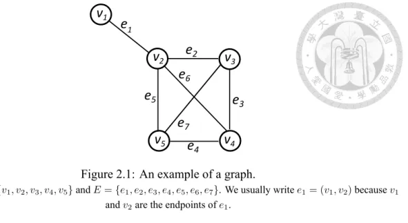
Definition 1. A graph G = (V, E) is a triple consisting of a vertex set V (G), an edge set E(G),

and a relation that associates with each edge two vertices called endpoints.

We write e = (u, v) for an edge e with endpoint u and v, and we say vertices u and v are adjacent if u and v are the endpoints of an edge, and that the edge is incident to u and to v.

Figure 2.1 gives an example of a graph.

Definition 2. The degree of a vertex v in a graph G, written degG(v) or simply deg(v), is the number of edges incident to v. The maximum degree of a graph G is ∆(G) = max_v_{∈V (G)}deg(v).

The neighborhood of v, written N_G(v) or simply N (v), is the set of vertices adjacent to v.

The closed neighborhood of a vertex v, written N_G[v] or simply N [v], is the vertex set containing v and N (v). The closed degree of a vertex, written deg[v], is defind to be|N[v]|;

and the maximum closed degree of a graph G is ∆^∗ = maxv∈V (G)|N[v]|

₆

Figure 2.1: An example of a graph.

It shows V ={v1, v₂, v₃, v₄, v₅} and E = {e1, e₂, e₃, e₄, e₅, e₆, e₇}. We usually write e1= (v₁, v₂) because v1

and v2are the endpoints of e1.

Hypergraphs Since our algorithms are implemented on hypergraphs, we introduce the definitions for hypergraphs below.

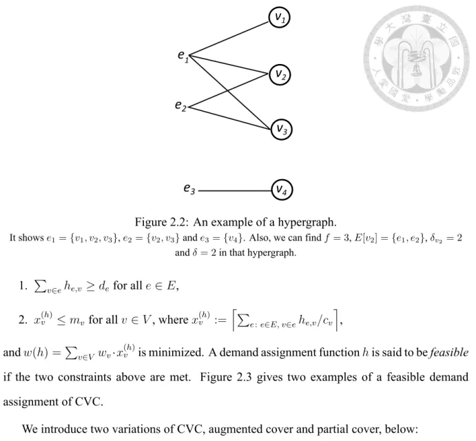
Definition 3. A hypergraph H = (V, E ⊆ 2^V) is a generalization of a graph where V is a set of vertices, and E is a set of non-empty subsets of V called hyperedges or edges.

Let f denote the maximum size of the edge set in a hypergraph H. E[v] denotes the set of hyperedges incident to v, and δ_v =|E[v]| is the vertex degree of a vertex v ∈ H. The maximum vertex degree of a hypergraph H is δ = max_v_{∈V (G)}|E[v]|. Figure 2.2 gives an example of a hypergraph.

2.2 The Capacitated Vertex Cover Problem

In this problem, we are given a hypergraph H = (V, E) where each e ∈ E is associated with a demand d_e ∈ R^≥0 and each v ∈ V is associated with a weight(or cost) wv ∈ R^≥0, a capacity c_v ∈ R^≥0, and an available multiplicity m_v ∈ Z^≥0. The demand of an edge is the amount of service it requires. The capacity of a vertex v is the amount of service each multiplicity of that vertex can provide to e∈ E[v].

The objective is to find a vertex multiset, or, cover, represented by a demand assignment function h : E× V → R^≥0, such that the following two constraints are met:

It shows e1={v1, v₂, v₃}, e2={v2, v₃} and e3={v4}. Also, we can find f = 3, E[v2] ={e1, e₂}, δv2= 2 and δ = 2 in that hypergraph.

1. ∑

v∈eh_e,v≥ de for all e∈ E,

2. x^(h)v ≤ mv for all v ∈ V , where x^(h)^v :=⌈∑

e : e∈E, v∈eh_e,v/c_v

⌉ , and w(h) =∑

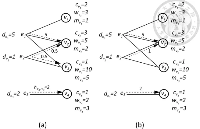
v∈V w_v·x^(h)v is minimized. A demand assignment function h is said to be feasible if the two constraints above are met. Figure 2.3 gives two examples of a feasible demand assignment of CVC.

We introduce two variations of CVC, augmented cover and partial cover, below:

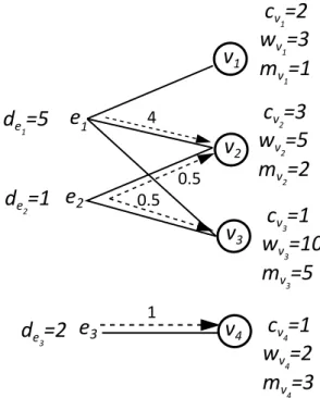
Augmented Cover. We relax the limit of multiplicity of each vertex to λ ≥ 1 times that of the vertex and find a feasible cover.

Definition 4. Let Π = (V, E, d_e, w_v, c_v, m_v) be an instance for HCVC. For any integral λ ≥ 1, we say that a demand assignment h forms a (λ, γ)-augmented-cover if

1. ∑

v∈eh_e,v ≥ defor all e∈ E.

2. x^(h)v ≤ λ · mv for all v∈ V .

3. w(h)≤ γ · minh^′∈Fw(h^′), whereF is the set of feasible demand assignments for Π.

Figure 2.4 gives an example of an augmented cover.

_e

1

=5 d

_e

2

=1

d

_e

_v

4

=3

h_e

3 ,v₄=2 0.5

5

0.5

(a)

1

=5 d

_e

2

=1

d

_e

₂

v

₃

v

₄

v

₁

e

1

e

₃

e

₂

d

_e

1

=5

d

_e

2

=1

d

_e

_v

4

=3

2 5

0.5 0.5

Figure 2.4: An example of an augmented cover with λ = 3.

If λ = 3, the available multiplicity of v1becomes 3· mv1 = 3 and the total capacity of v1is increased to 6. Thus de₁can be assigned to v1.

(25)

Partial Cover. We relax the covered demand to assure that at least L demand or β-fraction of total demand is covered. Another possible way of partially serving the demand is to serve α < 1 portion of demand for each edge. However, this type of partial cover problem for H can be reduced to a full cover problem for H’ as follows. Let H’ = H, except that the demand for each edge e’∈ H’ is set as de^′∈H^′ = αd_efor each edge e∈ H.

Definition 5. Let Π = (V, E, d_e, w_v, c_v, m_v) be an instance for HCVC. For any 0 ≤ β ≤ 1, a demand assignment h is said to be β-feasible if

∑

e∈E

min {

d_e,∑

v∈e

h_e,v }

≥ β ·∑

e∈E

d_e, and x^(h)_v ≤ mv for all v ∈ V.

LetF1 denote the set of 1-feasible demand assignments. We say that a demand assignment h forms a (β,γ)-partial-cover if h is β-feasible and w(h)≤ γ · minh^′∈F1w(h^′).

_e

1

=5

d

_e

2

=1

d

_e

_v

4

=3

1 4

0.5 0.5

Figure 2.5: An example of a partial cover with ϵ = 0.25.

If ϵ = 0.25, the covered demand is at least 6 in this hypergraph.

(26)

2.3 The Models of CVC

In this section, major categories of CVC models are introduced. These categories are discussed in the following subsections.

2.3.1 Parameter Conditions

Multiplicity condition. Depending on whether the available multiplicity of each vertex is limited, the work on CVC falls mainly in two categories: (1) soft capacity (SCVC), where the multiplicity of each vertex is unlimited, and (2) hard capacity (HCVC), where the available multiplicity of each vertex is limited.

Demand condition. Most papers solved CVC for graphs with unit edge demand (UD) first and then dealt with graphs with general edge demand (GD). From these results, the demand condition doesn’t seem to affect the approximation result in a significant way.

Weight condition. For simplification, the weight of all vertices, without loss of generality, is set to be one for unweighted (UW) version of the problem. On the other hand, for weighted (W) version, the weights of all vertices are arbitrary.

The weight condition significantly affects the complexity. For example, Chuzhoy and Naor [6] gave a 3-approximation for unweighted HCVC, and showed that the weighted version of HCVC is at least as hard as the set cover problem. Due to this reason, subsequent works on HCVC have mainly focused on the unweighted version.

2.3.2 Relaxation Constraints

The two variations of CVC are augmented cover (to relax the constraint on the limit of multi- plicity of each vertex) and partial cover (to relax the constraint about the covered demand).

(27)

2.3.3 Graph Type

The CVC is usually considered on simple graphs (SG), multigraphs (M), hypergraphs (HG), planar graphs (PG) or trees (T).

2.4 The Capacitated Domination Problem

The capacitated domination problem is an alternative notion of capacitated vertex cover prob- lem. For the capacitated domination problem, we are given a graph G = (V, E) with weight (or cost) w_v, capacity c_v, multiplicity m_v and demand d_v defined on each vertex. The demand of vertex v can be assigned to v’s closed neighbors, and the objective is to find a feasible demand assignment function such that the total weight is minimized. The demanding degree of v is the number of v’s closed neighbors with non-zero demand and ∆_dis the maximum demanding de- gree of G. There are two different models for the demand assignment. By inseparable demand model, we require that all the demand of a vertex v should be assigned to only one of its closed neighbors u ∈ N[v]. By separable demand model, the demand of a vertex can be assigned to several of its closed neighbors.

(28)

(29)

Chapter 3 The Overview of Capacitated Vertex Cover Problem

In this chapter, we give an overview of the proposed methods for CVC, and summarize related research works for SCVC, HCVC and other variations in recent years.

3.1 Methods

There are two main methods to solve CVC, namely, primal-dual schema and rounding. Both of them are based on the linear programming (LP) of CVC. The LP given in LP (3.1) below shows an example for SCVC with unit edge demand on simple graphs. There are two sets of variables, h_e,v and x_v, which correspond to the demand assignment function and the multiplicities of the vertices, respectively.

(30)

Minimize ∑

v∈V

w_v· xv (3.1)

h_e,v+ h_e,u ≥ 1, ∀e = {u, v} ∈ E c_v· xv− ∑

e∈E[v]

h_e,v ≥ 0, ∀v ∈ V

x_v − he,v ≥ 0, ∀e ∈ E, v ∈ e

h_e,v ∈ {0, 1}, ∀e ∈ E, v ∈ e

x_v ∈ N0 ∀v ∈ e

The first inequality states that the demand of each edge has to be fully-served. The second inequality connects the multiplicity function and the demand assignment function. The third inequality, which states that the multiplicity of a vertex cannot be zero if some demand is assigned to that vertex, is introduced to bound the integrality gap of the relaxation.

Primal-Dual Schema. The dual linear program of the relaxation of LP (3.1) is given in LP (3.2). There are three sets of variables y_e, z_v, and g_e,v, which can be interpreted as a packing program as follows. By primal-dual schema, the value of y_e is raised for all e∈ E. However, the value of each y_e is constrained by z_v and g_e,v that are further constrained by w_v for each v ∈ e. So zvand g_e,vwill be raised by the designed rule until the inequality related to w_v is met with equality, for which we say that the vertex v is saturated. Then the approximation result is obtained with the proposed demand assignment algorithm.

Primal-Dual Schema is usually applied in SCVC. For HCVC, there is the fourth set of mi- nus variables in the dual linear program (see LP (4.2)), which complicates the structure of the packing program in that it allows to pack even more values into y_ein the cost of a deduction in the objective value. This provides a certain degree of flexibility, and handling this flexibility

(31)

would be one of the major challenges for this problem.

Maximize ∑

e∈E

y_e (3.2)

c_v· zv + ∑

e∈E[v]

g_e,v ≤ wv, ∀v ∈ V

ye ≤ zv + ge,v, ∀v ∈ V, e ∈ E[v]

y_e, z_v, g_e,v, ≥ 0, ∀v ∈ V, e ∈ E[v]

Rounding. Rounding method is applied more widely than primal-dual schema. For SCVC, the results are the same using these two methods. And most of existing results for HCVC are built on the same two-staged rounding principle: First, it begins with a vertex-side threshold rounding. Then one or multiple edge-vertex patching procedure is introduced to meet the covering guarantee. The main challenge of this approach has been on devising a delicate patching procedure. To take the above LP as an example, the algorithm using rounding techniques usually follows the steps below:

1. Solve the LP to obtain an optimal fractional solution.

2. Pick a value α uniformly at random in the given interval [a, b].

3. For each edge e = (u, v) if h_e,u ≥ α then set h^∗e,u= 1, else if h_e,v ≥ α then set h^∗e,v = 1.

4. For the remaining edges (where he,u < α and he,v < α), these assignment function would be rounded up or down by a chosen probability with some patching process.

With elegant patching process, many improved approximations are obtained. Although the near-tight 2.155-approximation is obtained on simple graphs [5], it seems that current two- staged rounding techniques have reached their limitations, and significant new ideas are re- quired to close the gap.

(32)

Iterative Partial Rounding Scheme is designed by Kao [13] to close the gap. In each itera- tion, it makes partial decisions based on current working LP and rounds the demand assignment function fractionally, instead of rounding up the variables aggressively to one. When no such decisions are there to be made, it rounds up all vertices unconditionally and stops. Iterative partial rounding scheme improves the limitation of current two-staged rounding and Kao closed the gap of HCVC.

Others. There are a few other approaches employed for the problem, e.g., local ratio technique, extreme point method, the knapsack problem, iterative greedy method and fixed parameter tractable algorithm. We list these approaches below.

Local Ratio Technique is based on the Local Ratio Theorem [2] which chooses the greatest efficiency vertex iteratively.

Extreme Point Method is to analyse on the extreme points of the natural LP and a strength- ened LP lower-bound is obtained for the optimal solutions.

The Knapsack Problem: For CVC on trees, the demand assignment procedure can be re- duced to the knapsack problem and the approximation factor is bounded.

Iterative Greedy Choice is a greedy algorithm. In each iteration, the greatest efficiency vertex v, i.e. the vertex with largest effectiveness-cost ratio ( e.g. v ←− arg max{cv/w_v}), is chosen and the demand of incident edges is assigned to the vertex v.

Fixed Parameter Tractable Algorithm: The capacitated domination problem is W [1]-hard when parameterized by treewidth and solution size [14], so fixed parameter tractable algorithm is applied with respect to treewidth and the maximum capacity of the vertices.

3.2 Literature Survey

In this section, different works of CVC are described in more detail.

(33)

Model

Approximation Ratio Method Authors and Year Graph Demand

SG UD 2

Primal-Dual Schema Guha et al.

2002;2003

GD 3

HG UD f

GD f + 1

SG UD 2 Randomized Rounding Gandhi et al. 2002

Table 3.1: The summary of results of SCVC

3.2.1 Soft Capacity

The CVC with soft capacity was first introduced by Guha et al. [11]. They presented a 2- approximation for the case of unit edge demand on simple graphs based on primal-dual schema.

The LP and dual is given in LP (3.1) and LP (3.2). To maintain dual feasibility of the edge constraints y_e≤ zv+g_e,v, as they increase y_e, they increase z_vif the number of unassigned edges currently incident on vertex v is bigger then c_v, otherwise they increase g_e,v. The approximation factor becomes 3 with non-unit edge demand. These results extend to f -hypergraphs (each edge in the hypergraph is a subset of at most f vertices) with approximation factors of f and f + 1, respectively. They also proved that CVC on trees is NP-hard by a reduction from the Knapsack Problem. Gandhi et al. [8] proposed another 2-approximation via randomized rounding with unit edge demand. They improved approximation algorithms for throughput maximization in broadcast scheduling, delay minimization in broadcast scheduling, and capacitated vertex cover by the technique of dependent randomized rounding in bipartite graphs. In Table 3.1, we give a summary of results of SCVC.

The Capacitated Domination Problem Because the capacitated domination problem is an alternative notion of capacitated vertex cover problem, Kao et al. [14–17] studied capacitated dominating set problem and presented a series of results for the complexity and approximability of this problem.

Kao et al. [16] considered capacitated domination problem and proposed a ∆^∗-approximation algorithm using primal-dual schema. For trees, they gave a linear-time algorithm with inseparable demands and showed that this problem is NP-hard followed by the presentation of a

(34)

Model (Graph) Approximation Ratio Method Authors and Year

SG ∆^∗

Primal-Dual Schema

Kao et al. 2011 3

T PTAS Relaxed Knapsack Problem

P Constant Factor Primal-Dual Schema Kao et al. 2011

SG Logarithmic Greedy Choice

Kao et al. 2015

P 80 Primal-Dual Schema

Table 3.2: The summary of results of the capacitated domination problem

polynomial-time approximation scheme (PTAS) with separable demands by a fully polynomial- time approximation scheme (FPTAS) for the Relaxed Knapsack Problem.

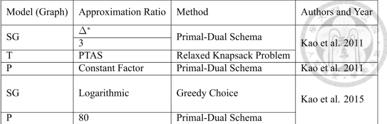
Kao and Lee [15] provided the first constant factor approximation on planar graphs. The al- gorithm is based on a perspective on the hierarchical structure, called General Ladder, of outer- planar graphs with primal-dual schema, and then extended to planar graphs. Kao et al. [14] presented logarithmic approximations with respect to both separable and inseparable demand mod- els on general graphs by iterative greedy choice. They gave a ln n-approximation for inseparable demand, and for separable demand model, they gave (2 ln n + 1)/(4 ln n + 2)-approximation algorithms for unweighted/weighted version. They also proved that this problem is W [1]-hard when parameterized by treewidth and solution size, regardless of demand assigning model.

Then they presented an exact fixed parameter tractable (FPT) algorithm for both demand models with respect to treewidth and the maximum capacity of the vertices. For planar graphs, they presented pseudo-polynomial-time approximation schemes for both demand models and proved a lower bound of (³₂ − ϵ) for the approximation ratio of any algorithm for planar graphs with inseparable demands, for any ϵ > 0, by the reduction from Partition, which is a well-known combinatorial problem that is known to be weakly NP-hard [9]. For separable demand model, they gave an 80-approximation algorithm by primal-dual schema under a standard framework due to Baker [1]. In Table 3.2, we show a summary of results of the capacitated domination problem.

(35)

3.2.2 Hard Capacity

For hard capacities, Chuzhoy and Naor [6] considered HCVC with unit demand. For unweighted HCVC, they gave a 3-approximation using randomized rounding with a specific patching procedure. They showed that the weighted version of HCVC is at least as hard as the set cover problem. Due to this reason, subsequent work on HCVC has focused on the unweighted version. For weighted capacitated set cover with unit demand, they presented a (ln δ + 1)- approximation by iterative greedy choice, where δ is the maximum size of the sets. This ap- proach further extends to a (ln max_Sf (S) + 1)-approximation for submodular set cover, which was proved by Wolsey [25]. Gandhi et al. [7] proposed a refined approach to [6] for unweighted HCVC with unit edge demand and obtained a 2-approximation. They added a preprocessing step in which they fixed the number of copies of certain capacity-1 vertices. After fixing the number of copies of these vertices they solved the relaxation of the integer linear program followed by randomized rounding. They also modify their alteration step that helps to bound the cost of the alteration step in a better way. Saha and Khuller [22] considered unweighted HCVC with general edge demands on multigraphs using randomized rounding. They provided a 34- approximation for the case of unit multiplicity and a 38-approximation for general multiplicities.

They also considered f -hypergraphs and proposed a max{6 · f, 65}-approximation. Recently, these results were improved by Cheung et al. [5], who provided a(

1 + 2/√ 3)

-approximation for general graphs and a 2· f-approximation for f-hypergraphs with unit demand. Their algorithms consist of a two-step process, each based on rounding an appropriate linear program.

In particular, for multigraphs, the analysis in the second step relies on identifying a matching structure within any extreme point solution. Kao et al. [17] gave a (∆_d+ 2)-approximation for unweighted capacitated domination problem with hard capacities by primal-dual schema. This result can be converted to a (δ + 2)-approximation for unweighted HCVC. We present it in sec- tion 4.3 Recently, Kao [13] presented an f -approximation for any f ≥ 2 and closed the gap of approximation for this problem. Kao provided a new rounding method, called Iterative Partial Rounding Scheme. In contrast to other rounding method, in which every vertex is rounded up with decent value at once, he only dealt with those that are structurally supported. Furthermore,

(36)

Model

Approximation Ratio Method Authors and Year Graph Demand Weight

SG UD UW 3 Randomized

Rounding

Chuzhoy and Naor 2002;2006 W At least as hard as the

set cover problem

SG UD UW 2 Randomized

Rounding Gandhi et al. 2003

MG GD UW 38 Randomized

Rounding

Saha and Khuller 2012

HG GD UW max{6 · f, 65}

MG UD UW (

1 + 2/√ 3)

Randomized

Rounding Cheung et al. 2014

HG UD UW 2f

HG GD UW δ + 2 Primal-Dual

Schema Kao et al.2015

HG GD UW f Iterative Partial

Rounding Kao 2017 Table 3.3: The summary of results of HCVC

instead of rounding up the variables aggressively to one, he rounded them partially to a fractional value by imposing stronger lower bound constraints on them. In Table 3.3, we give a summary of results of HCVC.

3.2.3 CVC with Relaxed Constraints

In this section, we review the related works for two variations of CVC, augmented cover and partial over.

Augmented Cover

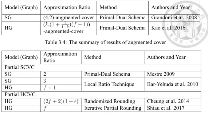
For augmented multiplicity constraints in weighted version, the proposed solutions in the literature all use primal-dual schema but use different approaches to raising variables in the dual linear program in their algorithms. Grandoni et al. [10] gave a (4,2)-augmented-cover for sim- ple graphs, which can be further extended to (f²,f )-augmented-cover for f -hypergraphs. By their algorithm, they raised just the variable g_e,v in each iteration. Kao et al. [18] improved it to (k,(1 + _1+k¹ )(f − 1))-augmented-cover for f-hypergraphs. Their variable raising policy is similar to that given in Guha et al. [11]. We show a summary of results of augmented cover in Table 3.4.

(37)

Model (Graph) Approximation Ratio Method Authors and Year SG (4,2)-augmented-cover Primal-Dual Schema Grandoni et al. 2008 HG (k,(1 + _1+k¹ )(f − 1))

-augmented-cover Primal-Dual Schema Kao et al. 2016 Table 3.4: The summary of results of augmented cover

Model (Graph) Approximation

Ratio Method Authors and Year

Partial SCVC

SG 2 Primal-Dual Schema Mestre 2009

SG 3

Local Ratio Technique Bar-Yehuda et al. 2010

HG f + 1

Partial HCVC

HG (2f + 2)(1 + ϵ) Randomized Rounding Cheung et al. 2014

HG f Iterative Partial Rounding Shiau et al. 2017

Table 3.5: The summary of results of partial cover Partial Cover

For partial SCVC, a 2-approximation for simple graphs was given by Mestre [21], based on a delicate primal-dual scheme developed for a gradually strengthened LP of this problem. This result can be extended to an f -approximation for hypergraphs. Bar-Yehuda et al. [4] presented a 3-approximation for simple graphs and (f + 1)-approximation for hypergraphs based on local ratio techniques and a specially designed charging scheme.

For partial HCVC for f -hypergraphs, Cheung et al. [5] gave a (2f +2)(1+ϵ)-approximation which runs polynomial in (|V |^1/ϵ|E|) time. They proposed a generic reduction from partial HCVC for f -hypergraphs to HCVC for (f + 1)-hypergraphs, with a small loss in the approxi- mation factor. Shiau et al. [23] improved it to a tight f -approximation using iterative rounding technique and a generalized analysis on the extreme points of the natural LP. We give a summary of results of augmented cover in Table 3.5.

(38)

(39)

Chapter 4 The Capacitated Vertex Cover Problem with Relaxed Constraints

In this chapter, we present our methods, algorithms and results about CVC. We use primal-dual with local charging scheme to solve a series of the HCVC problems. For unweighted version, we have a (δ + 2)-approximation algorithm. And for weighted version, we have obtained the following:

1. (k, (1 + _k₋₁¹ )(f − 1))-augmented-cover, which means we relax the multiplicity limit for a factor of k ≥ 2 and have a (1 +_k₋₁¹ )(f − 1)-approximation algorithm.

2. (1− ϵ, O(1/ϵ)f)-partial-cover for partial HCVC, which means the demand served is at least the ratio of 1− ϵ and we have an O(1/ϵ)f-approximation algorithm.

4.1 LP Relaxation and the Dual LP

Let Π = (V, E, d_e, w_v, c_v, m_v) be an input instance of HCVC. A natural LP relaxation of HCVC for an instance Π is given below in LP (4.1). There are two sets of variables, h_e,vand x_v, which correspond to the demand assignment function and the multiplicities of the vertices, respectively.

(40)

Minimize ∑

v∈V

w_v· xv (4.1)

∑

v∈e

h_e,v ≥ de, ∀e ∈ E

cv· xv − ∑

e∈E[v]

he,v ≥ 0, ∀v ∈ V

x_v ≤ mv, ∀v ∈ V

de· xv − he,v ≥ 0, ∀e ∈ E, v ∈ e

x_v, h_e,v ≥ 0, ∀e ∈ E, v ∈ e

The first inequality states that the demand of each edge has to be fully-served. The second inequality connects the multiplicity function and the demand assignment function. The third inequality places a constraint on the multiplicity of each vertex. The fourth inequality, which states that the multiplicity of a vertex cannot be zero if some demand is assigned to that vertex, is introduced to bound the integrality gap of the relaxation.

The dual linear program of the relaxation of LP (4.1) is given in LP (4.2). There are four sets of variables y_e, z_v, g_e,v, and η_v, which can be interpreted as a packing program as follows.

We want to raise the values of y_efor all e∈ E. However, the value of each yeis constrained by zv and ge,vthat are further constrained by wv for each v ∈ e.

(41)

Maximize ∑

e∈E

d_e· ye − ∑

v∈V

m_v· ηv (4.2)

c_v· zv + ∑

e∈E[v]

d_e· ge,v − ηv ≤ wv, ∀v ∈ V

y_e ≤ zv + g_e,v, ∀v ∈ V, e ∈ E[v]

y_e, z_v, g_e,v, η_v ≥ 0, ∀v ∈ V, e ∈ E[v]

The fourth set of variables, η_v, complicates the structure of the packing program in that it allows us to pack even more values into y_e because the raising of η_v offsets the raising of z_v. This presents a major challenge to bound the total cost given by our primal-dual schema.

4.2 A Primal-Dual Schema for HCVC

In this section, we present our extended primal-dual algorithm for HCVC. The algorithm that we present extends the framework developed for the soft capacity model [11, 16]. In the prior framework, the demand is assigned immediately as soon as the cost for these vertices is charged to the dual variables corresponding to the adjacent edges. In our algorithm, we keep some of decisions of demand assignment pending until we have sufficient capacity for the demands. In contrast to the primal-dual scheme used in [10], which always raises dual values in g_e,v, we raise the dual values g_e,vand z_v, depending on the amount of residual demand that v possesses in its incident edges. This ensures that, the cost of each multiplicity of a vertex is charged only to the demands that it serves.

To obtain a solid bound for this approach, however, we need to ensure that the vertices whose multiplicity limits are attained receive sufficient amount of demands to charge to. This motivates our flow-based procedure Self-Containment to make sure that we have sufficient

(42)

capacity for the demands for dealing with the pending decisions. During this procedure, a natural demand assignment is also made. We present our primal-dual algorithm in §4.2.1 and its analysis in §4.2.2.

4.2.1 The Algorithm

We present our extended primal-dual algorithm Dual-HCVC below. This algorithm takes as input an instance Π = (V, E, d, w, c, m) of HCVC and outputs a feasible primal demand as- signment h together with a feasible dual solution Ψ = (y_v, z_v, g_e,v, η_v) for Π.

The algorithm starts with an initial zero dual solution and eventually reaches a locally optimal solution. During the process, the values of the dual variables in Ψ are raised gradually and some inequalities will meet with equality. We say that a vertex v is saturated if the inequality c_v· zv+∑

e∈E[v]d_e· ge,v− ηv ≤ wv is met with equality.

Let E^ϕ :={e : e ∈ E, de > 0} be the set of edges with non-zero demand and V^ϕ :={v : v ∈ V, mv · cv > 0} be the set of vertices with non-zero capacity. For each v ∈ V , we use d^ϕ(v) = ∑

e∈E[v]∩E^ϕd_e to denote the total amount of demand in E[v]∩ E^ϕ. For intuition, E^ϕ contains the set of edges whose demands are not yet processed nor assigned, and V^ϕcorresponds to the set of vertices that have not yet been saturated.

In addition, we maintain a set S, initialized to be empty, to denote the set of vertices that have been saturated and that have at least one incident edge in E^ϕ. Intuitively, S corresponds to vertices with pending assignments.

The algorithm works as follows. Initially all dual variables in Ψ and the demand assignment h are set to be zero. We raise the value of the dual variable y_efor each e∈ E^ϕsimultaneously at the same rate. To maintain the dual feasibility, as we increase y_e, either z_v or g_e,v has to be raised for each v ∈ e. If d^ϕ(v)≤ cv, then we raise g_e,v. Otherwise, we raise z_v. In addition, for all v ∈ e ∩ S, we raise ηv to the extent that keeps v saturated.

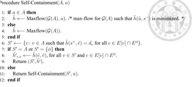
When a vertex u ∈ V^ϕ becomes saturated, it is removed from V^ϕ. Then we invoke a recursive procedure Self-Containment(S∪{u}, u), which is a flow-based procedure, to compute

(43)

a pair (S^′, h^′), where

• S^′is a maximal subset of S∪ {u} whose capacity, if chosen, can fully-serve the demands in E[S^′]∩ E^ϕ, and

• h^′ is the corresponding demand assignment function (from E[S^′]∩ E^ϕto S^′).

If S^′ = ∅, then we leave the assignment decision pending and add u to S. Otherwise, S^′ is removed from S and E[S^′] is removed from E^ϕ. In addition, we add the assignment h^′ to final assignment h to be output. This process repeats until E^ϕ = ∅. Then the algorithm outputs h and Ψ and terminates. A pseudo-code for this algorithm can be found in Figure 4.1.

We also note that, the particular vertex to saturate in each iteration is the one with the smallest value of w^ϕ(v)/ min{cv, d^ϕ(v)}, where w^ϕ(v) := wv− (cv· zv+∑

e∈E[v]de· ge,v− ηv) denotes the current slack of the inequality associated with v ∈ V^ϕ.

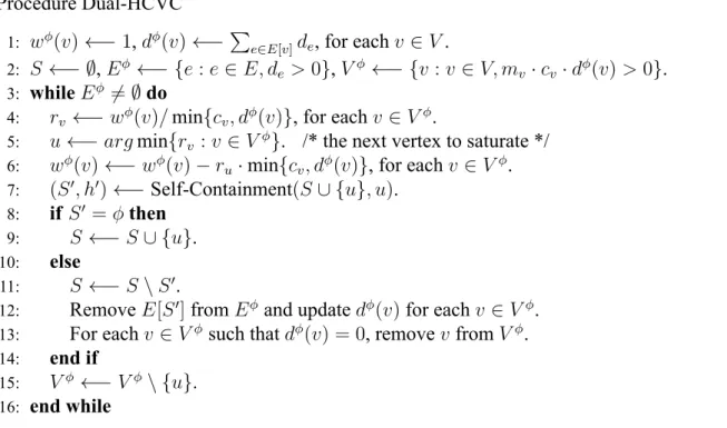
Procedure Dual-HCVC

1: w^ϕ(v)←− 1, d^ϕ(v)←−∑

e∈E[v]d_e, for each v ∈ V .

2: S ←− ∅, E^ϕ←− {e : e ∈ E, de > 0}, V^ϕ ←− {v : v ∈ V, mv· cv· d^ϕ(v) > 0}.

3: while E^ϕ̸= ∅ do

4: r_v ←− w^ϕ(v)/ min{cv, d^ϕ(v)}, for each v ∈ V^ϕ.

5: u←− arg min{rv : v ∈ V^ϕ}. /* the next vertex to saturate */

6: w^ϕ(v)←− w^ϕ(v)− ru· min{cv, d^ϕ(v)}, for each v ∈ V^ϕ.

7: (S^′, h^′)←− Self-Containment(S ∪ {u}, u).

8: if S^′ = ϕ then

9: S ←− S ∪ {u}.

10: else

11: S ←− S \ S^′.

12: Remove E[S^′] from E^ϕand update d^ϕ(v) for each v ∈ V^ϕ.

13: For each v ∈ V^ϕsuch that d^ϕ(v) = 0, remove v from V^ϕ.

14: end if

15: V^ϕ←− V^ϕ\ {u}.

16: end while

Figure 4.1: A pseudo-code for our Dual-HCVC process.

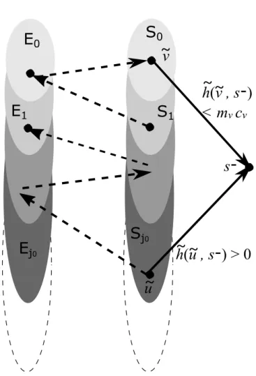
The Procedure Self-Containment(A, u). In the following we describe the recursive proce- dure Self-Containment(A, u). It takes as input a vertex subset A⊆ V and a vertex u ∈ V and

有容量的點覆蓋問題在放寬條件下之可近似性

國立臺灣大學電機資訊學院資訊工程學系 博士論文

Department of Computer Science and Information Engineering College of Electrical Engineering and Computer Science

National Taiwan University Doctoral Dissertation

有容量的點覆蓋問題在放寬條件下之可近似性 The Approximability of Capacitated Vertex Cover Problem

with Relaxed Constraints

杜海倫 Hai-Lun Tu

指導教授：李德財院士 Advisor: D.T. Lee, Academician

中華民國 108 年 1 月

January 2019

Acknowledgements

摘要

Abstract

Contents

List of Figures

List of Tables

Chapter 1 Introduction

1.1 Motivation

1.2 Background

1.3 Our Contributions

1.4 Organization of this Dissertation

Chapter 2

Definitions and Notation

2.1 Fundamental Graph Theory

v

v

v

v

v

e

e

e

e

e

e

e

2.2 The Capacitated Vertex Cover Problem

v

v

v

v

e

e

e

v

v

v

v

e

e

e

d

=5 d

=1

d

=2

c

=2 w

=3 m

=1 c

=3 w

=5 m

=2 c

=1 w

=10 m

=5 c

=1 w

=2 m

=3

(a)

v

v

v

v

e

e

e

d

=5 d

=1

國立臺灣大學電機資訊學院資訊工程學系博士論文