國立臺灣大學電機資訊學院電信工程學研究所 碩士論文
Graduate Institute of Communication Engineering College of Electrical Engineering and Computer Science
National Taiwan University Master Thesis
K-頻段輻射計量測及近場成像
K-band Radiometer Measurement and Near-Field Imaging
蔡昱墩 Yu-Tun Tsai
指導教授:瞿大雄 博士 Advisor: Tah-Hsiung Chu, Ph.D.
中華民國 106 年 7 月
July 2017
中文摘要
本論文係依據普朗克黑體輻射定律,使用 K 頻段輻射計量測物體產生之雜訊 功率。第一章介紹輻射計基本原理,第二章敘述輻射計之天線及接收機中頻及射頻 模組量測結果,並計算天線解析度及接收機等效雜訊溫度。第三章第一節敘述接收 機連接 20 dB 導波管天線為一輻射計,量測 50 負載、吸收體、鋁板及人手之雜 訊功率,並計算物體之雜訊溫度。第二節則敘述接收機連接 85 cm 碟形天線為一輻
射計,並安裝於二維平面掃描器,量測 1.38 公尺距離之近場物體 18 公分 18 公
分所計算之雜訊功率,量測數值經 Visual Basic 程式控制及量測,並以 MATLAB 程式顯示物體之成像,量測物體包含吸收體、20 dB 增益天線之輻射低功率以及發 熱之陶瓷電阻。
Abstract
In this thesis, a K-band radiometer is developed to measure the noise power coming from an object based on Plank’s blackbody radiation law. The basic radiometer theory is briefly introduced in Chapter 1. The measured results of a 85 cm dish antenna, IF and RF stages of a receiver are presented in Chapter 2 to give the antenna spatial resolution and receiver noise temperature. In Sec. 3.1 of Chapter 3, the receiver is connected with a 20 dB horn antenna as a radiometer to measure the noise power of four different objects to calculate their noise temperatures. In Sec. 3.2.2, a radiometer is developed to connect the receiver and a 85 cm dish antenna. The radiometer is mounted on a 18 cm 18 cm scanner as a near-field imaging system to measure the noise power from the test object at 1.385 m distance. The recorded result and image are controlled through a personal computer using Visual Basic and MATLAB programs. The near-field imaging several objects includes a low-power antenna, absorber and heated ceramic resistors.
Table of Contents
口試委員會審定書 ... #
中文摘要 ... i
Abstract ... ii
Table of Contents ... iii
List of Figures ... v
List of Tables ... viii
Chapter 1 Basic Theory ... 1
1.1 Brightness and Brightness Temperature ... 1
1.2 Equivalent Noise Temperature and Noise Figure ... 2
1.3 Antenna ... 5
1.3.1 Antenna Temperature... 5
1.3.2 Spatial Resolution ... 7
1.4 Receiver ... 8
1.5 Detection and Integration ... 10
Chapter 2 Radiometer Measurements ... 12
2.1 Antenna Near-Field Measurement ... 12
2.2 Receiver Measurement ... 20
2.2.1 RF Stage ... 20
2.2.2 IF Stage ... 23
2.2.3 Receiver ... 26
Chapter 3 Noise Power and Near-Field Imaging Measurements ... 32
3.1 Noise Power Measurements ... 32
3.2 Near-Field Imaging Measurements ... 36
3.2.1 Cable behind LNA Case ... 39
3.2.2 Cable after LNA Case ... 42
Chapter 4 Conclusion ... 46
References ... 47
Appendices ... 49
1.1 Measurement Program Using Visual Basic ... 49
1.2 Imaging Program Using MATLAB ... 62
List of Figures
Fig. 1.1 Radiometer consists of an antenna and a receiver. ... 1 Fig. 1.2 A lossy network with matched source and load. ... 4 Fig. 1.3 Spatial resolution on x-axis by moving (a) an antenna with x to give two (b)
unresolved, (c) just resolved, and (d) resolved patterns. ... 7 Fig. 1.4 (a) Receiver block diagram with (b)~(f) corresponding to each operational
spectrum. ... 9 Fig. 2.1 (a) Dish antenna, (b) NSI2000 near-field antenna measurement arrangement,
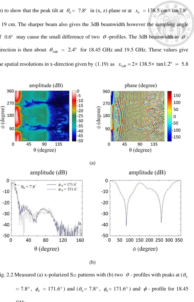
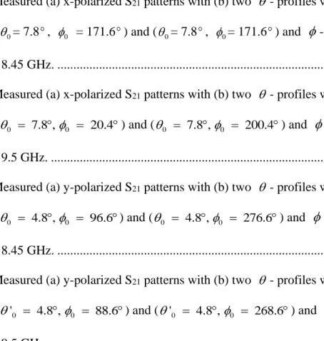
(c) its photograph and (d) coordination. ... 13 Fig. 2.2 Measured (a) x-polarized S21 patterns with (b) two - profiles with peaks at
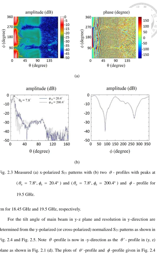
( = 7.80 , = 171.60 ) and ( = 7.80 , = 171.60 ) and - profile for 18.45 GHz. ... 15 Fig. 2.3 Measured (a) x-polarized S21 patterns with (b) two - profiles with peaks at
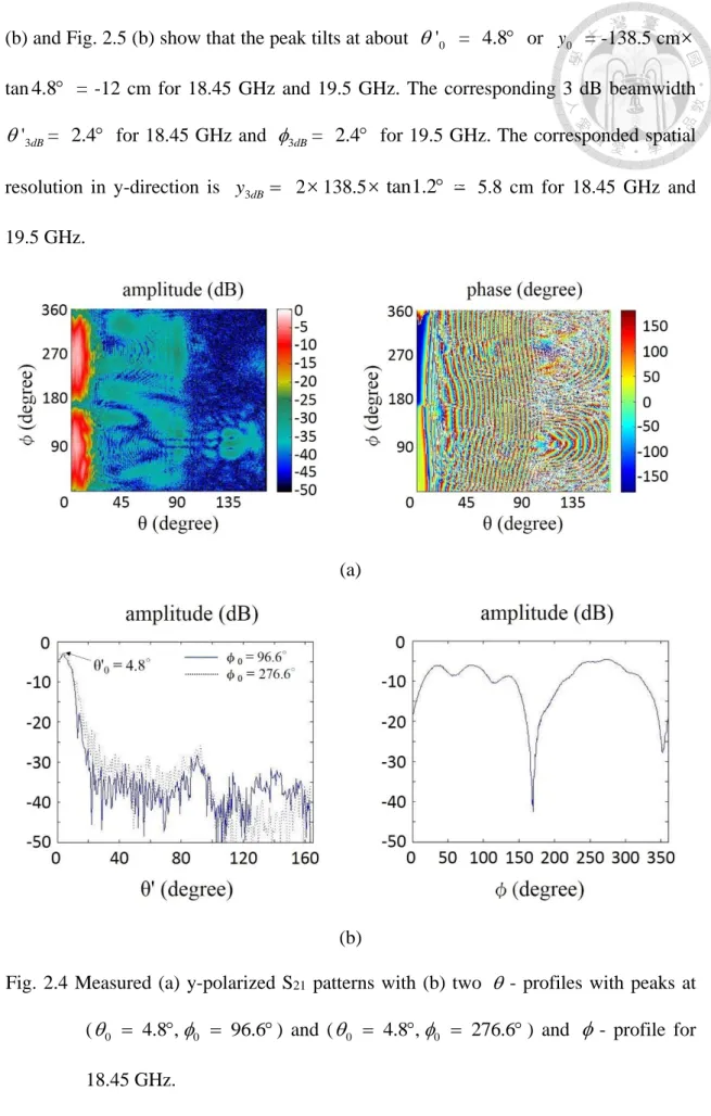
(0 7.8 , 0 20.4) and (0 7.8 , 0 200.4) and - profile for 19.5 GHz. ... 16 Fig. 2.4 Measured (a) y-polarized S21 patterns with (b) two - profiles with peaks at
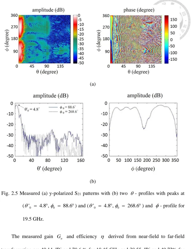
(0 4.8 , 0 96.6) and (0 4.8 , 0 276.6) and - profile for 18.45 GHz. ... 17 Fig. 2.5 Measured (a) y-polarized S21 patterns with (b) two - profiles with peaks at
('0 4.8 , 0 88.6) and ('0 4.8 , 0 268.6) and - profile for 19.5 GHz. ... 18 Fig. 2.6 Measured x-polarized holograms at z = 1.385 m for (a) 18.45 GHz and (b)
19.5 GHz. ... 19
Fig. 2.7 Measured far-field patterns at (a) 18.45 GHz and (b) 19.5 GHz. ... 20
Fig. 2.8 RF stage measurement arrangement. ... 21
Fig. 2.9 Measurement results of (a) a 30 dB attenuator and (b) noise figure and conversion gain of RF stage. ... 22
Fig. 2.10 IF stage measurement arrangements for (a) 1.2 GHz and (b) 150 MHz. ... 24
Fig. 2.11 Measured results of (a) a 70 dB attenuator, noise figure and gain of IF stage at (b) 1.2 GHz and (c) 150 MHz. ... 26
Fig. 2.12 Measurement arrangements of receiver for (a) 18.45 GHz and (b) 19.5 GHz. 27 Fig. 2.13 Measurement results of receiver noise figure and gain for (a) 18.45 GHz and (b) 19.5 GHz. ... 29
Fig. 2.14 Arrangement to compensate two attenuators 2 for the noise figure measurement. ... 30
Fig. 3.1 (a) Measurement arrangement and (b) its graphical user interface. ... 33
Fig. 3.2 Photographs of noise power measurement including (a) an absorber, (b) an aluminum plate, (c) a hand and (d) a 50 load. ... 34
Fig. 3.3 (a) Measurement arrangement and (b) its photograph. ... 37
Fig. 3.4 (a) Observed planes and (b) graphical user interface. ... 38
Fig. 3.5 Photographs of four objects including (a) an excited horn antenna, (b) absorber piles, (c) an aluminum plate and (d) a 250W lamp... 40
Fig. 3.6 Imaging results of (a) a low-power excited horn antenna and (b) absorber plies. ... 40
Fig. 3.7 Imaging results of (a) aluminum plate and (b) 250W lamp. ... 42
Fig. 3.8 (a) The LNA is connected after the dish horn and (b) its larger view. ... 42
Fig. 3.9 (a) A 20 dB horn antenna and (b) its imaging result. ... 43
Fig. 3.10 (a) Absorbers piles and (b) imaging result. ... 43
Fig. 3.11 (a) Photograph of ceramics resistors and (b) its circuit with IR
measured temperature values. ... 44 Fig. 3.12 (a) Heated ceramic resistors and (b) imaging result. ... 45
List of Tables
Table 2.1 Measured results of parabolic dish antenna. ... 19
Table 2.2 Setting values of PNA N5222A for RF stage measurement. ... 21
Table 2.3 Measurement results of noise figure and conversion gain of RF stage. ... 23
Table 2.4 Setting values of PNA 5222A for IF stage measurement. ... 24
Table 2.5 Measurement results of IF stage. ... 24
Table 2.6 Setting values of PNA5222A for receiver measurement. ... 28
Table 2.7 Receiver measurement results. ... 29
Table 3.1 Measurement results of noise power for four objects. ... 34
Chapter 1 Basic Theory
The objective of radiometer is to passively measure the noise power generated by the object brightness, to be explained in Sec. 1.1, in microwave region. Radiometer hardware basically consists of an antenna and a low noise with high gain receiver as illustrated in Fig. 1.1. The antenna is to collect the object radiation. The receiver is used to amplify the antenna received noise then detect and integrate the measured noise power.
There are few radiometer parameters involved. They include spatial resolution, integration time, and temperature resolution, which is also the radiometer sensitivity.
These terminologies will be discussed later in Chapter 2.
Fig. 1.1 Radiometer consists of an antenna and a receiver.
1.1 Brightness and Brightness Temperature
All natural objects whose temperatures are above absolute 0 K can emit electromagnetic energy. They also absorb and scatter the electromagnetic energy incident on them. In thermal equilibrium, a perfect absorber that absorbs all the incident energy and does not reflect is called a blackbody. According to Kirchhoff’s law of radiation, a perfect absorber emits the energy as the same as it absorbs. The radiation from a blackbody source is given by Planck’s law as [1]
3
2 /
2 1
1.
rad hf kT
B hf
c e
(1.1)
In (1.1) c 3108 m/s is the speed of light. f is frequency in Hz. h = 6.6310-34 J
s is Planck’s constant. k = 1.3810-23 J is Boltzmann’s constant. T in K is the absolute temperature of the blackbody. Brad in W m-2 Hz-1 is the radiation emitted by the blackbody and is also called brightness or brightness spectral density.
For microwaves in K-band from 18 GHz to 26 GHz, hf is much smaller than kT, therefore, one can use the first two terms of the Taylor series expansion approximation as
/ 1
hf kT hf
e kT (1.2)
or the Rayleigh-Jeans approximation to give (1.1) as
2
2
rad
B kT
(1.3)
where is the wavelength. When the object is not a blackbody, it partially reflects the incident energy. The measured brightness is smaller than that given in (1.3). Therefore the brightness temperature TB is defined as TBeT [2] where e is the object emissivity with 0 e 1 and depends on the body material. The object brightness Brad is then given as
2 2
2 2
rad B .
k k
B T eT
(1.4)
It indicates the brightness temperature distribution TB( , ) measured by a microwave radiometer can give a spatial description of the object observed in microwave region. This work has been developed in radio astronomy for years [3].
1.2 Equivalent Noise Temperature and Noise Figure
Planck’s blackbody radiation law can also be applied to electronic circuits. The following description is referred from [4]. The electronic components generate energy which is called thermal noise. Considering a resistor at physical temperature of T K, the
electrons in the resistor are in random motion, with a kinetic energy that is proportional to the temperature. This energy produces a random voltage across the resistor given by
/
4 .
n hf kT 1
V hfR
e
(1.5)
Vn in (1.5) is the root mean square value of random voltage spectrum in Volt Hz-1. R is the resistance in . By using (1.2) with f in K-band, (1.5) can be simplified as
4 .
Vn kTR (1.6)
This noisy resistor has the maximum power transfer when its load is matched to a resistor with the same value. The power spectrum delivered to the load is
2
2 .
4
n n
P V R kT
R (1.7)
Since the above noise power is independent of frequency, it has a power spectral density being constant with frequency. The noise power is then directly proportional to the bandwidth and given as
Pn kTB (1.8)
where B is the operational bandwidth. The noisy resistor is called a white noisy resistor.
For an arbitrary noisy source or network where noise power (thermal or nonthermal) is not strongly dependent of frequency over the bandwidth of interest, it can be characterized with an equivalent noise temperature as
o.
e
T N
kB (1.9)
In (1.9), No is the noise power delivered to a matched load.
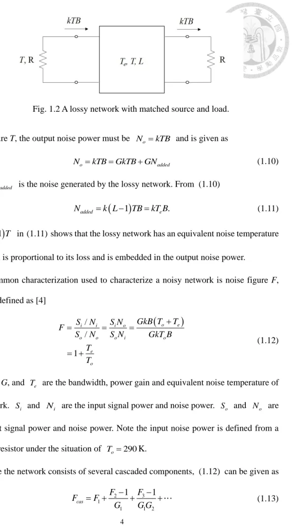
Consider a lossy network having power loss of L and it matches with source and load resistors at temperature T as shown in Fig. 1.2. The loss factor L is given by L = 1/G > 1 with G being the power gain. Since the entire system is in thermal equilibrium at the
Fig. 1.2 A lossy network with matched source and load.
temperature T, the output noise power must be No kTB and is given as
o added
N kTBGkTBGN (1.10)
where Nadded is the noise generated by the lossy network. From (1.10)
1
.added e
N k L TBkT B (1.11)
1
Te L T in (1.11) shows that the lossy network has an equivalent noise temperature Te which is proportional to its loss and is embedded in the output noise power.
A common characterization used to characterize a noisy network is noise figure F, which is defined as [4]
/ / 1
o e
i i i o
o o o i o
e
o
GkB T T S N S N
F S N S N GkT B
T T
(1.12)
Where B, G, and Te are the bandwidth, power gain and equivalent noise temperature of the network. Si and Ni are the input signal power and noise power. So and No are the output signal power and noise power. Note the input noise power is defined from a matched resistor under the situation of T o 290K.
Once the network consists of several cascaded components, (1.12) can be given as
2 3
1
1 1 2
1 1
cas
F F
F F
G G G
(1.13)
where Fcas is the overall noise figure. F1, F2, F3, G1, and G2 are the noise figure and gain of each component. The form of the overall equivalent noise temperature Tcas is then
2 3
1
1 1 2
e e
cas e
T T
T T
G G G
(1.14)
where Te1, Te2 and Te3 are the equivalent noise temperature of each component. For a cascaded system with high gain in each component, Fcas and Tcas are dominated by the characteristics of the first stage.
1.3 Antenna
The purpose of radiometer antenna is to effectively collect the brightness radiating from the observed object temperature. It connects to a radiometer receiver to measure the noise power.
1.3.1 Antenna Temperature
When an antenna points toward an object with the spatial distribution of brightness temperature TB
, given by (1.4), its received power spectrum Pr in WHz-1 is given by [1]
2
1 2 , ,
r 2 B r
P kT A d
(1.15)where
, 2
, , .
r
r
a r m
A d
A P
A
(1.16)
In (1.16), Ar
, is the receiving antenna cross section and2
r m 4 a
A G
is the maximum receiving antenna cross section with Ga being the antenna gain. Pa
, is the normalized receiving antenna radiation power pattern. The factor 12 is because the antenna receives only one polarization and the integral is overall the solid angle. Given the operation bandwidth B, the normalized received power against the background can then be written as
, ,
,
B a
r a
a
T P d
P k B kT B
P d
(1.17)where Ta is called the antenna temperature. The antenna output power Pr is usually expressed in terms of its antenna temperature Ta. It is obvious that the antenna received noise power is an integral of the object brightness temperature seen by the antenna multiplying the antenna radiation power pattern over the observation range. This thesis then uses this equation to give the image of the observed object brightness temperature
,TB by having the antenna radiation pattern to be a delta function at a certain direction
0, 0
. In our experiment, a parabolic dish antenna with 85 cm diameter is used.For a realistic antenna with dissipative loss, the antenna received power is reduced by the antenna efficiency , which is the ratio of the antenna output power to the input rad power. The received object brightness temperature will also be reduced by the factor of
. Note the thermal noise is generated by the antenna loss can be modeled as a lossless rad
antenna with a loss of L1/rad. The resulted antenna noise temperature TA is given by [5]
1
p
1
a
A rad a rad p
L T
T T T T
L L
(1.18)
where Tp is the antenna physical temperature. Hence the antenna noise temperature TA is a linear combination of the antenna temperature Ta related to the observed object brightness temperature TB
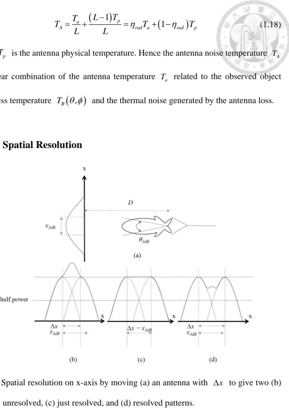
, and the thermal noise generated by the antenna loss.1.3.2 Spatial Resolution
Fig. 1.3 Spatial resolution on x-axis by moving (a) an antenna with x to give two (b) unresolved, (c) just resolved, and (d) resolved patterns.
Consider an antenna points to an object as shown in Fig. 1.3 (a) and the distance between antenna and object is D. The curve on the x-axis represents the magnitude of the antenna main beam projection. is half power beamwidth and 3dB x3dB is the projected width corresponding to with a distance of D. The spatial resolution along x-axis is 3dB
given by
3
3 2 tan
2
dB
xdB D
(1.19)
If the antenna is moved by x, which is smaller than x3dB, as shown in Fig. 1.3 (b), peaks of the original pattern (dotted lines) cannot be distinguished in the combined pattern (solid line), which is called the unresolved pattern. Once x is greater thanx3dB, as shown in Fig. 1.3 (d), two peaks can be distinguished from the combined pattern and they are resolved. For xis equal to x3dB, as shown in Fig. 1.3 (c), two patterns are just resolved. x3dB is then called the spatial resolution of the antenna along x-axis.
In our experiment, the parabolic dish antenna is moved in a planar scanner. The antenna spatial resolution in x-direction is then determined by in -direction. 3dB Similarly, one can define the antenna spatial resolution y3dB in cross x-direction (or y- direction).
1.4 Receiver
Once the object radiating noise power or antenna temperature is received by the antenna, the receiver then provides a very high gain about 100 dB with a low noise figure.
The noise power level for an object at 290 K observed by a receiver with bandwidth of 30 MHz is about No 290 Kk 30 MHz 1.210-10 mW = -99.2 dBm based on (1.8). The receiver amplification is provided over the RF and IF stages and the noise figure is determined by the receiver RF stage.
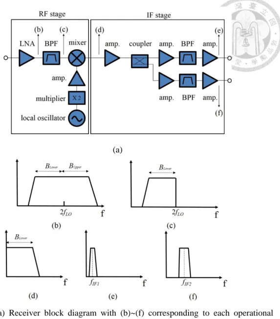
Fig. 1.4 (a) shows the block diagram of the receiver used in this thesis. The RF stage consists of a broad band low noise amplifier (LNA) and a bandpass filter to extract the lower sideband of the signal after LNA. The local oscillator provides a sinusoidal output,
(a)
Fig. 1.4 (a) Receiver block diagram with (b)~(f) corresponding to each operational spectrum.
whose frequency fLO = 9.825 GHz is doubled by a frequency multiplier and then amplified by an amplifier. A mixer is used to down convert the frequency from RF band to IF band. In IF stage, an IF amplifier increases the signal from the RF stage. A coupler offers a pair of signal paths and the signal in each path is amplified and filtered to fIF1 and fIF2 frequencies. This receiver was used for the ROCSAT-1 communication experiment [6] as a beacon receiver with fIF1 = 150 MHz and a communication receiver for fIF2 = 1.2 GHz. The corresponding RF frequency channels are 19.5 GHz and 18.45
GHz.
The receiver frequency allocation is presented in Fig. 1.4 (b)~(f) and the measured results will be given in the next Chapter. Fig. 1.4 (b) shows the LNA output spectrum, where BLower is the lower sideband and BUpper is the upper sideband. Fig. 1.4 (c) shows the output spectrum of bandpass filter in RF stage, whose upper sideband is removed. Fig.
1.4 (d) shows the mixer output spectrum. Fig. 1.4 (e) and (f) show the output spectra of the IF stage for two paths at fIF1 and fIF2.
1.5 Detection and Integration
To measure the observed noise power, a square-law detector is used through its property of diode nonlinearity. The diode output voltage is proportional to the receiver output power. From (1.9) and (1.18), the diode output voltage can be expressed as [2]
A rec rec rec
rec
V kT BG kT BG CP
(1.20)
In (1.20) TA is the antenna noise temperature. Trec is the receiver equivalent noise temperature. B and Grec are the receiver bandwidth and power gain. C is the factor for the receiver measured output noise power to be given in Chapter 3.
Because TA and Trec are random signals, V presents extremely high fluctuation.
Therefore, an integrator smooths the random signal by averaging in a specific time of . The longer integration time gives more smoothed value of V. It then needs more bandwidth to give more smoothed result. The temperature resolution or sensitivity of a radiometer is then given as [2]
.
A rec
sys
T T
T B
T B
(1.21)
As long as 1 B is large enough, the measured equivalent temperature after the integrator is close to Tsys. It is the summation of antenna noise temperature and receiver noise temperature. The object brightness temperature is embedded in the antenna noise temperature given by (1.17). Higher value of bandwidth and integration time will then increase the measurement accuracy.
In this thesis, the detection and integration is realized by using an Agilent U2000A power sensor. In the next Chapter, detail description of measured results of antenna and receiver will be presented to given receiver B, Grec, Trec and antenna , spatial resolution, pointing direction
0, 0
and gain G . Chapter 3 then gives noise power a measurements of radiometer for several objects. The corresponded antenna noise temperature TA and antenna temperature Ta will then be calculated.Chapter 2 Radiometer Measurements
In Chapter 1, (1.19) depicts that antenna spatial resolution corresponds to antenna beamwidth. In order to have a resolution in cm, antenna should have high gain with small 3dB beamwidth. In addition, receiver should have low noise figure in order to have low Trec. This chapter will present the measurement results of antenna, RF stage and IF stage of receiver. The measured receiver result also gives the value of bandwidth B, determined by the IF stage, to calculate integration time. In addition, the measured antenna results give antenna main beam pointing angle, spatial resolution and efficiency.
2.1 Antenna Near-Field Measurement
In this thesis, a parabolic dish antenna with 85 cm diameter used in ROCSAT-1 experiment [6] is shown in Fig. 2.1 (a) to give a small spatial resolution. The wooden support is used to fix a horn antenna, Continental Microwave PA42-8, with about 8 dB gain. The horn is operated at TE10 mode with linear polarization in x-direction as shown in Fig 2.1 (b) and (d). Its frequency range is in K-band from 18 to 26.5 GHz.
(a)
(b)
(c) (d)
Fig. 2.1 (a) Dish antenna, (b) NSI2000 near-field antenna measurement arrangement, (c) its photograph and (d) coordination.
Fig. 2.1 (b) and (c) is the NSI2000 [7] near-field antenna measurement arrangement and its photograph. A dual linear polarized log pyramidal receiving probe antenna, NSI- RF-DLP-03, at the top of an arm moved in -direction to give a circular trace in (x , z) plane in Fig. 2.1 (d). The range of is from to 165 and the radius r is 1.385 0 m. For each angle, the parabolic dish antenna is rotated in -direction to give a circular path in (x, y) plane. The range of is from to 360. The movement 0 then gives two linear polarized near-field radiation patterns of the parabolic dish antenna on a spherical coordinate with radius of 1.385 m through switching the polarization of receiving probe at x- and y-directions. The moving step of - and -rotations is set at
0.6 . The test frequency is set from 16 GHz to 20 GHz with a step of 0.5 GHz. An Agilent PNA-L N5232A is used to measure S21 values at the specified frequency between the receiving probe connected at port 2 and the parabolic dish antenna connected at port 1 at Fig. 2.1 (b). Note the two jumper at port 2 are properly changed to increase the receiver dynamic range by 15 dB [8].
Fig 2.2 and Fig. 2.3 show the measured x-polarized (or co-polarized) normalized S21
values given by the solid lines at frequencies of 18.45 GHz and 19.5 GHz. The distance of 1.385 m will be used later in the near-field imaging measurements for that between the parabolic dish antenna and the imaged object to be given in the next chapter. Both the amplitude patterns given in Fig 2.2 (a) and Fig 2.3 (a) indicate the parabolic antenna has a sharp tilted main beam by the solid lines at 0 7.8 and 0 171.6 for 18.45 GHz and 0 7.8 and 0 20.4 for 19.5 GHz. Since -direction corresponds to the rotation of parabolic dish antenna, the patterns at 0180 given in Fig. 2.2 (b) and Fig. 2.3 (b) basically repeat the same x-polarization. The plots of maximum -profile are at (0 7.8 , 0 351.6) and (0 7.8 , 0 200.4 ) in Fig 2.2 (b) and Fig 2.3
(b) to show that the peak tilt at = 0 7.8 in (x, z) plane or at x = 138.5 cm0 tan7.8
= 19 cm. The sharper beam also gives the 3dB beamwidth however the sampling angle of 0.6 may cause the small difference of two -profiles. The 3dB beamwidth in - direction is then about 3dB = 2.4 for 18.45 GHz and 19.5 GHz. These values give the spatial resolutions in x-direction given by (1.19) as x3dB 2138.5tan1.2 5.8
(a)
(b)
Fig. 2.2 Measured (a) x-polarized S21 patterns with (b) two - profiles with peaks at (0
= 7.8, = 171.60 ) and ( = 7.80 , = 171.60 ) and - profile for 18.45 GHz.
(a)
(b)
Fig. 2.3 Measured (a) x-polarized S21 patterns with (b) two - profiles with peaks at (0 7.8 , 0 20.4 ) and (0 7.8 , 0 200.4 ) and - profile for 19.5 GHz.
cm for 18.45 GHz and 19.5 GHz, respectively.
For the tilt angle of main beam in y-z plane and resolution in y-direction are determined from the y-polarized (or cross-polarized) normalized S21 patterns as shown in Fig. 2.4 and Fig. 2.5. Note -profile is now in -y-direction as the '- profile in (y, z) plane as shown in Fig. 2.1 (d). The plots of -profile and ' -profile given in Fig. 2.4
(b) and Fig. 2.5 (b) show that the peak tilts at about '0 = 4.8 or y = -138.5 cm0 tan4.8 = -12 cm for 18.45 GHz and 19.5 GHz. The corresponding 3 dB beamwidth
'3dB
= 2.4 for 18.45 GHz and 3dB= 2.4 for 19.5 GHz. The corresponded spatial
resolution in y-direction is y3dB 2138.5tan1.2 5.8 cm for 18.45 GHz and 19.5 GHz.
(a)
(b)
Fig. 2.4 Measured (a) y-polarized S21 patterns with (b) two - profiles with peaks at (0 4.8 , 0 96.6 ) and (0 4.8 , 0 276.6 ) and - profile for 18.45 GHz.
(a)
(b)
Fig. 2.5 Measured (a) y-polarized S21 patterns with (b) two - profiles with peaks at ('0 4.8 , 0 88.6 ) and ('0 4.8 , 0 268.6 ) and - profile for 19.5 GHz.
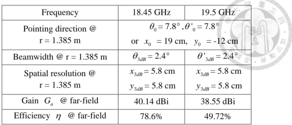
The measured gain G and efficiency a derived from near-field to far-field transformation are 40.14 dBi and 78.6 % for 18.45 GHz and 38.55 dBi and 49.72% for 19.5 GHz. The gain values are close to those of [6]. Table 2.1 summarizes the main beam pointing direction, beamwidth, spatial resolution, gain and efficiency of the 85 cm parabolic dish antenna.
Frequency 18.45 GHz 19.5 GHz Pointing direction @
r = 1.385 m
= 7.8 ,0 = 7.8 '0 or x = 19 cm, 0 y = -12 cm 0 Beamwidth @ r = 1.385 m 3dB= 2.4 '3dB= 2.4
Spatial resolution @ r = 1.385 m
x3dB= 5.8 cm y3dB= 5.8 cm
x3dB= 5.8 cm y3dB= 5.8 cm Gain G @ far-field a 40.14 dBi 38.55 dBi Efficiency @ far-field 78.6% 49.72%
Table 2.1 Measured results of parabolic dish antenna.
The main beam direction can also be verified from the holograms shown in Fig. 2.6 and the far field pattern shown in Fig. 2.7. Fig. 2.6 (a) and (b) show the measured x- polarized holograms at the distance of z = 1.385 m. The peak is shown close to x = 10 o cm and y = -10 cm which is close to the pointing direction given in Table 2.1. The 0 color scale is in dB. The spatial resolution in x- and y-direction are about x3dB = 5 cm and y3dB = 5 cm. The dashed square with a range of 20 cm20 cm will be the scanning range in the near-field imaging measurement to be presented in the next Chapter. The far
(a) (b)
Fig. 2.6 Measured x-polarized holograms at z = 1.385 m for (a) 18.45 GHz and (b) 19.5 GHz.
field pattern calculated from the measured near field data is shown in Fig. 2.7 for 18.45 GHz and 19.5 GHz. The pointing angles are at about (0 3 ,0 7.5 ) and (0 3 , ). The beam pointing angles are close to that given in Table 2.1. The 0 5 tilt of the main beam is due to the mislocations of horn antenna and back support of parabolic dish antenna as shown in Fig. 2.1 (c).
(a) (b)
Fig. 2.7 Measured far-field patterns at (a) 18.45 GHz and (b) 19.5 GHz.
2.2 Receiver Measurement
In this section, noise figure and power gain of receiver RF and IF stages are measured by an Agilent 4-port PNA N5222A. The two jumpers at port 2 of PNA are also properly changed to bypass the directional coupler to get 15 dB more power for the PNA receiver at port 2 as that given in Fig. 2.1 (b) [8].
2.2.1 RF Stage
The measurement arrangement for RF stage is shown in Fig. 2.8. The input and output ports of IF stage are terminated with 50 terminations. Since the RF stage has input P1dB -30 dBm [9], a 30 dB attenuator is connected at the RF stage input to
Fig. 2.8 RF stage measurement arrangement.
Frequency range 17.65 GHz to 19.64 GHz
Port 1 power level -13 dBm
IF bandwidth 600 kHz
Noise bandwidth 1.2 MHz
Average value 400
Ambient temperature 293.6 K
Table 2.2 Setting values of PNA N5222A for RF stage measurement.
prevent the RF stage from saturation. It also improves the RF stage input match to accommodate the match requirement of (1.7). The receiver DC bias is at 12 V and 0.748 A. PNA N5222A is operated under the “noise figure converters” measurement class using the cold source method [10] to measure the conversion gain and noise figure.
The setting values of PNA are given in Table 2.2. The frequency range is from 17.65 GHz to 19.64 GHz to give the IF frequency range from 10 MHz to 2 GHz. The input signal power level is -13 dBm to make sure that the RF stage and the PNA receiver at port 2 are operated in linear range. The local oscillation frequency of the RF stage is 19.65 GHz. The setting values of PNA noise bandwidth and average value are properly
(a)
(b)
Fig. 2.9 Measurement results of (a) a 30 dB attenuator and (b) noise figure and conversion gain of RF stage.
given in Table 2.2 to smooth the measured noise figure value based on (1.21).
Fig. 2.9 (a) shows the measured attenuation of 30 dB attenuator is 31.8 dB. This value is used to compensate the measured conversion gain and noise figure as shown in
Fig. 2.9 (b). The noise figure is about 3.16 dB and 5.02 dB for 18.45 GHz and 19.5 GHz, respectively. The conversion gain is about 31.38 dB and 25.33 dB for 18.45 GHz and 19.5 GHz, respectively. Measured results of noise figure and conversion gain are shown in Table 2.3. The equivalent noise temperature TRF of RF stage is calculated from measured noise figure using (1.12).
Frequency 18.45 GHz 19.5 GHz
Noise figure 3.16 dB 5.02 dB
Conversion gain 31.38 dB 25.33 dB
TRF 310.34 K 631.29 K
Table 2.3 Measurement results of noise figure and conversion gain of RF stage.
2.2.2 IF Stage
As shown in Fig. 2.10, a 70 dB attenuator is connected between the port 1 of PNA N5222A and the input port of IF stage since the IF stage has input P1dB -61dBm [9].
The PNA is operated under the “noise figure cold source” measurement class and its setting values are shown in Table 2.4. The frequency range is from 10 MHz to 2 GHz.
(a)
(b)
Fig. 2.10 IF stage measurement arrangements for (a) 1.2 GHz and (b) 150 MHz.
Frequency range 10 MHz to 2 GHz
Port 1 power level -13 dBm
IF bandwidth 5 kHz
Noise bandwidth 1.2 MHz
Average value 400
Ambient temperature 293.5 K
Sweep average for noise figure 4
Table 2.4 Setting values of PNA 5222A for IF stage measurement.
Frequency 1.2 GHz 150 MHz
Noise figure 6.87 dB 12.58 dB
Gain 68.16 dB 70.01 dB
3 dB bandwidth 104.03 MHz 35.697 MHz
TIF 1120.58 K 4962.89 K
Table 2.5 Measurement results of IF stage.
The input signal power level is -13 dBm to ensure that the IF stage and the PNA receiver at port 2 are operated in linear region. The setting values of noise bandwidth and average value are the same as those in RF stage except the sweep average is 4 to smooth the noise figure values.
Measured results are shown in Fig. 2.11. Fig. 2.11 (a) is the measured attenuation of 70.5 dB of a 70 dB attenuator to compensate the measured gain and noise figure. The measured values of noise figure in Fig. 2.11 (b) and (c) are given with a multiplication factor of 1 11220184.54 due to compensating the 70 dB attenuator given as
70.5
1010 11220184.54. (2.1)
Measured results of noise figure, gain and bandwidth of the IF stage for 1.2 GHz and 150 MHz are given in Table 2.5. The equivalent noise temperature TIF is calculated from measured noise figure using (1.12). For 1.2 GHz channel, results of IF stage are NF = 6.87 dB, G = 68.16 dB and B = 104.03 MHz. For 150 MHz channel, results of IF stage are NF = 12.58 dB, G = 70.01 dB and B = 35.697 MHz.
(a)
(b)
(c)
Fig. 2.11 Measured results of (a) a 70 dB attenuator, noise figure and gain of IF stage at (b) 1.2 GHz and (c) 150 MHz.
2.2.3 Receiver
To ensure the receiver and the PNA port 2 receiver are operated in linear region, receiver input power should to be below -106 dBm. This value is given by considering
(a)
(b)
Fig. 2.12 Measurement arrangements of receiver for (a) 18.45 GHz and (b) 19.5 GHz.
the summation of the input P1dB= -30 dBm of the RF stage, the input P1dB= -61 dBm of the IF stage and additional 15 dB gain of the Agilent 5222A port 2 receiver by changing two jumpers. Since this power level is less than the noise power of -93.8 dBm at 290 K with B = 104.03 MHz, a 70 dB attenuator is connected before the RF stage and a 20 dB attenuator is connected between the RF stage and the IF stage as shown in Fig. 2.12. In the measurement, the 70.5 dB attenuation is compensated for noise figure as given in (2.1). More detail to compensate the 20 dB attenuator will be discussed later.
The setting values of PNA are shown in Table 2.6. Measured receiver results are shown in Fig. 2.13 and Table 2.7. For 1.2 GHz channel, NF = 5.89 dB to give Trec =
Frequency 18.45 GHz 19.5 GHz
Port 1 power level -10 dBm -16 dBm
IF bandwidth 600 KHz 10 MHz
Noise bandwidth 1.2 MHz 1.2 MHz
Average value 400 400
Ambient temperature 293.6 K 293.6 K
Sweep average 4 4
Table 2.6 Setting values of PNA5222A for receiver measurement.
(a)
(b)
Fig. 2.13 Measurement results of receiver noise figure and gain for (a) 18.45 GHz and (b) 19.5 GHz.
Frequency 18.45 GHz 19.5 GHz
Noise Figure 5.89 dB 7.97 dB
Gain Grec 96.98 dB 96.96 dB
3dB bandwidth B 103.15 MHz 34.539 MHz
Trec 835.64 K 1527.18 K
Table 2.7 Receiver measurement results.
835.64 K using (1.12), Grec = 96.98 dB and B = 103.15 MHz. For 150 MHz, NF = 7.97 dB to give Trec = 1527.18 K , Grec = 96.96 dB and B = 34.539 MHz.
As described earlier the noise figure measurement in Fig. 2.12 includes a 20 dB attenuator connected between the RF stage and the IF stage and it is included in the results of Table 2.7. The following procedure is then given to compensate or subtract its effect on the receiver noise figure.
Shown in Fig. 2.14, each component has power gain G and noise figure i NF . i Attenuation 1 represents a 70 dB attenuator and attenuator 2 represents a 20 dB
Fig. 2.14 Arrangement to compensate two attenuators 2 for the noise figure measurement.
attenuator. The second and forth components represent the RF stage and the IF stage. The overall noise figure Fcas is given by (1.13) as
2 3 4
1
1 1 2 1 2 3
2 3 4
1
1 1 1 2 1 2 1 2 3 1 2 3
2 3 4 3
1 1
1 1 2 1 2 1 2 3 1 2
1 1 1
1 1 1
1 .
cas
F F F
F F
G G G G G G
F F F
F G G G G G G G G G G G G
F F F L
F L
G G G G G G G G G G
(2.2)
Since noise figure of a attenuator equals to its loss given by F1 = L1 =
1
1 G and
3 3
1 2 1 2
F L
G G G G , (2.2) can be written as
4
1 2
2 2 3
1 .
cas
F G F F
G G G
(2.3)
With one more measurement with a different attenuator 2, additional (2.3) can be written as
4
1 2
2 2 3
' 1 .
cas '
F G F F
G G G
(2.4)
Subtracting (2.3) by (2.4) gives
1 3 34
2 3 3
' '
' .
cas cas
F F G G G
F
G G G
(2.5)
Subtracting (2.5) by (2.3) gives
1 32 1
2 3 3
' '
1 .
'
cas cas
cas
F F G G
F F G
G G G
(2.6)
Adding (2.5) and (2.6) then gives
1 3 3 1 3 3
4 2
2 3 3
' ' 1 ' 1
1 .
'
cas cas
G G F G G G F G
F F
G G G
(2.7)
If attenuator 2 has a large attenuation to give G3 1 and G3' 1, (2.7) can be approximated as
1 3 3
4 2
2 3 3
' '
1 .
'
cas cas
G G F G F
F F
G G G
(2.8)
The left term before the equal sign is the overall noise figure of stage 2 and stage 4 by compensating the effect of attenuators 2. However, the noise figure or Trec in Table 2.7 include the additional effect of the 20 dB attenuator.
Chapter 3 Noise Power and Near-Field Imaging Measurements
In this chapter, the measured parabolic dish antenna and receiver are integrated as a radiometer mounted on a two-dimensional scanner to give near-field imaging of several objects. In Sec. 3.1, the receiver is connected to a 20 dB horn antenna to measure the noise power values of four different objects. A program written using Visual Basic performs the measurements. Sec. 3.2 then describes the near-field imaging measurements.
Resulted images are displayed by a program using MATLAB. Both programs are given in the appendixes.
3.1 Noise Power Measurements
The measurement arrangement is shown in Fig. 3.1 (a). A horn antenna with 20 dB gain is connected at the receiver input to collect the brightness radiating from the observed objects. An Agilent U2000A power sensor [11] is connected at receiver output to detect and integrate the received noise power. A personal computer controls the integration time and record the noise power through a USB interface. The program is written using Visual Basic with the graphical user interface as shown in Fig. 3.1 (b).
The measurement procedure is given as the following.
(1) Click the selection listing and choose USB port.
(2) Click ON to connect the personal computer with the power sensor.
(3) Click Initialize and Zero to reset and calibrate power sensor when the receiver is power off.
(4) Click Status and VISA Read to receive the message to ensure the connection is
(a)
(b)
Fig. 3.1 (a) Measurement arrangement and (b) its graphical user interface.
done.
(5) Enter the operation frequency and integration time then click Measure. The first and averaged power values are displayed on the screen.
Fig. 3.2 (a)-(c) show the photographs of three different objects sensed by the receiver and a 20 dB horn antenna. They are an absorber, an aluminum plate and a hand. Fig. 3.2 (d) shows the photograph of a 50 load connected at the receiver input for reference.
(a) (b)
(c) (d)
Fig. 3.2 Photographs of noise power measurement including (a) an absorber, (b) an aluminum plate, (c) a hand and (d) a 50 load.
The integration time is set at 40 seconds and each object are measured 5 times.
Measurement results are listed in Table 3.1 with the receiver for four observed objects.
The noise power given by 18.45 GHz is higher than that of 19.5 GHz because its bandwidth is about 3 time, or about 5 dB wider with about the same receiver gain Grec. Noise power measured from aluminum plate is the lowest and human hand has the largest
IF frequency 18.45 GHz 19.5 GHz
Absorber 2.516 mW 4 dBm 1.150 mW 0.61 dBm
Aluminum plate 2.395 mW 3.79 dBm 0.674 mW -1.7 dBm
Hand 2.557 mW 4.07 dBm 1.171 mW 0.69 dBm
50 load 2.518 mW 4.01 dBm 1.148 mW 0.6 dBm
Table 3.1 Measurement results of noise power for four objects.
noise power. This is because aluminum plate has low emissivity and temperature of human hand is higher than others. The measurement results of absorber and 50 load are very close as expected.
Using (1.20), the noise temperature of the 50 load can be calculated as the reference with its physical temperature and measured results of receiver noise temperature, bandwidth and gain given in Table 2.7. Calculated noise power values for 50 load are 9.04 dBm ( assuming T50= Tp = T = a T = 292.5 K) using (1.20) A ( k(T + a Trec)BGrec = 1.3810-23( 292.5 + 835.64 )103106109.7103 = 8.04 mW = 9.05 dBm) for 18.45 GHz and 6.34 dBm (1.3810-23( 292.5 + 1527.18 )34.5
106109.7103 = 4.34 mW = 6.38 dBm) for 19.5 GHz. The values are higher than measured results of 50 load given in Table 3.1. The measured noise power values for 50 at 2.518 mW and 1.148 mW give equivalent noise temperatures Tsys= 353.46 K
( Nsys/kBGrec = 3
23 6 9.7
2.518 10 1.38 10 103 10 10
) for 18.45 GHz and Tsys = 481.12 K (=
3
23 6 9.7
1.148 10 1.38 10 34.5 10 10
) for 19.5 GHz. These measured noise temperature values are smaller than those of T + a Trec giving before. To calculate the factors in (1.20), the factor values of measured noise power to calculated noise power C = 0.313 (= 2.518 / 8.04) and C = 0.264 (= 1.148 / 4.34) for 18.45 GHz and 19.5 GHz. Therefore the measured noise temperature values of hand are given as 311 K =38 C (= 3
23 6 9.7
2.557 10
0.313 1.38 10 103 10 10
835.64
) and 332 K = 59 C (= 3
23 6 9.7
1.171 10
0.264 1.38 10 34.5 10 10
1527.18) for 18.45 GHz and 19.5 GHz.
Similarly the measured noise temperature values of aluminum plate are given as 238
K (= 3
23 6 9.7
2.395 10
0.313 1.38 10 103 10 10
835.64) and -457 K (= 3
23 6 9.7
0.674 10
0.264 1.38 10 34.5 10 10
1527.18)
for 18.45 GHz and 19.5 GHz. The calculated noise temperature of aluminum at 19.5 GHz is less than 0 K is not reasonable due to the multi-scattering of aluminum plate and horn antenna. The measured noise temperature values of absorbers are similar to those of 50
loads. The temperature resolution given by (1.21) is 0.018 K (( T + a Trec )/ B =
( 292.5 + 835.64 )/ 103 10 640) for 18.45 GHz and 0.049 K (( 292.5 + 1527.18 ) / 34.5 10 640) for 19.5 GHz.
As the objects move about few centimeters away from the 20 dB horn antenna, the values of measured noise power are the same. One reason is that the background noise may dominate the antenna noise temperature T due to wide antenna beamwidth. Note a that the contrast between absorber and aluminum plate at 19.5 GHz is higher than that of 18.45 GHz. The near-field measurements given in the next section is then performed at this frequency.
3.2 Near-Field Imaging Measurements
(a)
(b)
Fig. 3.3 (a) Measurement arrangement and (b) its photograph.
In this section the parabolic dish antenna and receiver including the power sensor are mounted on a Sigma Koki three-axis stage [12] as shown in Fig. 3.3 (a) and (b). The observed object is located about 1.385 m from the dish antenna tilt angle about 30 from the vertical (V) direction in Fig. 3.3 (a). The three-axis stage moves in vertical and horizontal (H) directions for 18 cm 18 cm facing to the observed plane. The cable connected between dish horn and receiver has 2.23 dB loss at 19.5 GHz. Later in Sec.
3.2.2 the LNA in RF stage will be connected to the dish horn directly to reduce the effect by cable loss. The power sensor is connected at the receiver 150 MHz output port.
Absorber piles are located as the background with 120 cm 90 cm area.
The radiometer moves with its scanning area facing to the observed area as depicted in Fig. 3.4 (a). The dashed-line square marked by H-axis and V-axis is the area corresponding to the physical center of the dish antenna. X-axis and y-axis are the axes corresponding to Fig. 2.6 (b) with about 30 tilt angle due to the attachment of the dish antenna mounting plate to the three-axis stage. The solid square represents the plane mapped to the estimated main beam of dish antenna as explained in Sec. 2.1. Its center is
(a)
(b)
Fig. 3.4 (a) Observed planes and (b) graphical user interface.
at about x = 10 cm and y = -10 cm as given in Fig. 2.6 (b).
A personal computer is used to control SHOT-204MS controller moving the three- axis stage in a raster scan, integrate the power sensor reading values and record the averaged noise power. The program given in Sec. 3.1 is then revised to include the control
of three-axis stage. The related graphical user interface is shown in Fig. 3.4 (b). The measurement procedure is given as the following.
(6) Repeat steps 1 to 4 as those given in Sec. 3.1.
(7) Select the port number and click RS232 ON.
(8) Click Robot Status and receive the character “R” to ensure the connection is done.
(9) Click Robot Initialize to initialize the stage.
(10) Enter operation frequency, integration time, start position, stop position and interval number then click Start to begin the measurement.
3.2.1 Cable behind LNA Case
In this section, the cable of 2.23 dB loss at 19.5 GHz is located between the dish horn and the receiver. The observed object is placed at point A in Fig. 3.4 (a). The scanning area is 18 cm 18 cm in a raster scan with a step of 1cm. The operating frequency is19.5 GHz and the integration time is 12 second. Four different objects are observed and their photographs are as shown in Fig. 3.5 (a)-(d).
Fig. 3.5 (a) is a 20 dB gain horn antenna excited with Hewlett Packard 8320A source connected through a 60 dB attenuator and a 2.5 dB loss cable to give a low-power about -72.8 dBm. The 20 dB horn antenna and is tilted to match the polarization of the dish
(a) (b)
(c) (d)
Fig. 3.5 Photographs of four objects including (a) an excited horn antenna, (b) absorber piles, (c) an aluminum plate and (d) a 250W lamp.
(a) (b)
Fig. 3.6 Imaging results of (a) a low-power excited horn antenna and (b) absorber plies.
horn. Fig. 3.5 (b) is absorber piles and Fig. 3.5 (c) shows an aluminum plate. Fig. 3.5 (d) is a 250W lamp and its temperature is about200 C . The resulted images are presented with gray scale in Fig. 3.6 using a display program written by MATLAB.
Shown in Fig. 3.6 (a) of a low-power indicates the radiometer gives a brighter image at the upper right side. This is because the antenna is placed near point A (8.72 cm, 8cm) as illustrated in Fig. 3.4 (a). The largest measured power is close to 1.8 mW assumed to be the noise power to give about equivalent noise temperature Tsys = 754.35 K.
Considering the factor of 0.264 given in Sec.3.1, the noise power is 6.82 mW (1.8 mW / 0.264 ) to give equivalent noise temperature of Tsys= 2857.4 K. To subtract the receiver noise temperature of Trec= 1527.18 K, the equivalent noise temperature is T = 1330.21 a K. The measured lowest noise power is about 1.4 mW to give about equivalent noise temperature of Tsys= 586.7 K. Similarly by considering the factor, the noise power is 5.3 mW to give Tsys = 2222.42 K and T = 693.24 K. a
Fig. 3.6 (b) is the image of absorber piles. The noise power values around 1.29 mW to give equivalent noise temperature of Tsys = 541 K are lower than the lowest temperature given in Fig. 3.6 (a). By considering of the factor of 0.264, the noise power is 4.89 mW to give Tsys= 2047.8 K and T = 520.62 K.The upper side is colder than the a lower side. This is because the scanning starts from the right lower corner. The absorber gradually turns into thermodynamic equilibrium to the surrounding temperature to give about measured noise power to be 1.27 mW. By considering the factor of 0.264, the noise power is 4.81 mW to give Tsys = 2016 K and T = 488.9 K (a 216 C ) to be compared with the results in Fig. 3.10 (b) in Sec. 3.2.2.
Fig. 3.7 (a) has the similar imaging result as Fig. 3.6 (b) because the brightness temperature of aluminum plate is low and it also reflects the surrounding brightness temperature. The imaging result of a 250W lamp depicts that it seems to be warmer at the upper side with about of measured noise power of 1.28 mW. However, the measured noise power values are close to those of the absorber piles. Note the 2.23 dB loss cable connected before the receiver increases the receiver noise figure ( and noise temperature Trec) to increase the object noise temperature. Based on this reason, the receiver noise power is reduced by placing the LNA before the cable and measurements are repeated.
(a) (b)
Fig. 3.7 Imaging results of (a) aluminum plate and (b) 250W lamp.
3.2.2 Cable after LNA Case
(a) (b)
Fig. 3.8 (a) The LNA is connected after the dish horn and (b) its larger view.
The cable of 2.23 dB loss is replaced with another cable having 1.36 dB loss. The LNA is removed from receiver and connect after the feed horn of dish antenna as shown in Fig. 3.8. The observed object is shown in Fig. 3.9 (a) a 20 dB horn antenna with input power of -74.53 dBm at 19.5 GHz slightly smaller than that in Fig. 3.5 (a). Note it is shifted to the left side of H-axis and placed at the point A’ (17.7 cm, 9 cm) in Fig. 3.4 (a).
The integration time is 5 second. Fig. 3.9 (b) shows the imaging result. The measured noise power values are smaller than those given in Fig. 3.6 (a). The resulted image is tilted to the left lower side because the horn antenna is shifted to point A’. The largest and
(a) (b)
Fig. 3.9 (a) A 20 dB horn antenna and (b) its imaging result.
(a) (b)
Fig. 3.10 (a) Absorbers piles and (b) imaging result.
lowest measured power are close to 1.7 mW and 1.1 mW to give Tsys= 2698.65 K and
Tsys=1746.19 K, and T = 1171.47 K and a T = 219 K by considering the same factor of a 0.264. The dynamic range of T is three times more than that in Fig. 3.6 (a) with LNA a inside the receiver.
Fig. 3.10 shows the observed absorber piles and imaging result. Integration time is 12 seconds and the temperature resolution is about 0.09K with Tsys = 1819.68 K by considering the factor of 0.264. Comparing with Fig. 3.6 (b), the measured noise power is lower with further variation, because the receiver noise figure is lower by the moving
![Fig. 2.1 (b) and (c) is the NSI2000 [7] near-field antenna measurement arrangement and its photograph](https://thumb-ap.123doks.com/thumbv2/9libinfo/9608459.634018/24.892.159.794.97.1174/fig-nsi-near-field-antenna-measurement-arrangement-photograph.webp)