介電致動高分子在崩潰電壓下與其材料可逆性的討論與研究

(1)

國立臺灣大學工學院機械工程學研究所碩士論文

Department of Mechanical Engineering College of Engineering

National Taiwan University Master Thesis

介電致動高分子在崩潰電壓下與其材料可逆性的討論與研究 Dielectric Electroactive Polymers at Breakdown Voltage State and

Reversibility

張致國

Chih-Kuo Chang

指導教授：施文彬博士 Advisor: Wen-Pin Shih, Ph.D.

中華民國 100 年 2 月

Feb, 2011

(2)

i

(3)

誌謝

兩年多的碩士生涯，不長不短的日子，豐富了我人生閱歷。有幸能加入微型機械力學實驗室，更有幸能有老師施文彬教授的指導；老師對研究嚴謹認真的態度、對研究內容新穎的看法，深深影響了我，於論文付梓之際，非常感謝老師，

在研究上的細心指導及生活上的關心，讓我裨益良多，對未來的人生態度更有其助益。

感謝宜蘭大學胡毓忠教授，中興大學戴慶良教授，高雄大學施博仁教授在百忙之中抽空擔任學生的口試委員，並給予學生在論文與研究上許多寶貴的建議，使拙著漸趨完備。

感謝微機械力學實驗室燿全、明道、冠緯、梁道、鐸儒、承俊、倬昱學長、

泊耕、光甫同學及子方、耿華、宗樺、品淳、承暾、其融、阿圓、渝淇、端明學弟們的協助與建議，都是我能持續努力的動力。在實驗室生活的點點滴滴，是我人生中難得的經驗。

感謝 CL 及 FE 還有成景會的每一個人，因為有了你們，讓我的求學生涯點綴得更加豐富；感謝一直支持我的韋麒、阿軒、swercy、黃平，因為你們，我有了繼續向前的動力。

最後我要感謝我的母親和姊姊，因為你們提供衣食無缺的環境，以及包容與體諒，讓我能沒有後顧之憂的完成碩士學業。如果沒有您們，就不會有現在的我，

對您們真的是滿滿的感激。特別要感謝我的女朋友飛飛，因為有你的陪伴，我才能走得更加有力、更加平順，對於未來也更有方向。

還有，我的父親，因為你，賦予論文更非凡的意義。

致國

(4)

摘要

近年來，由於介電致動高分子材料(dielectric electroactive polymers, DEAPs)具有良好的力學性質、高介電係數及低成本的特性，讓其在做為致動器的範疇中受到相當的注目。然而，介電致動高分子材料的驅動特性會受驅動電壓大小及其幾何尺寸上限制的影響；隨著電壓的上升，因所受靜電力增加而使上下電極逐漸靠近，若發生吸附效應則兩電極最終會貼合。若介電致動高分子材料厚度較薄，則可以降低驅動電壓，並提升材料的可靠度；材料可靠度的研究是近來重要的課題。

本論文針對材料崩潰現象、吸附現象及其可逆性進行探討。實驗中給予一直流電壓，觀察電流及變形量隨時間與不同驅動電壓的變化情形。實驗結果顯示當電壓加至 2000Ｖ時，會有大電流出現，象徵此時即為崩潰現象發生的時刻；並由已推知的條件判斷式可以得到崩潰現象會發生在吸附效應之前。本實驗同時經由逐漸增加電壓至 1600V，再降回 0V，觀察其材料的可逆與重複性，並對其遲滯效應做一些探討。另一方面，本論文也透過靜電及超彈性材料的力分析提出力電耦合的材料模型。

關鍵字：介電致動高分子材料、吸附效應、超彈性、崩潰現象、可逆性、理 論模型

(5)

Abstract

Recently, there has been growing interest in actuators by using dielectric electroactive polymers, DEAPs due to their attractive properties of mechanism, low cost and high dielectric constant. However, operating characteristics of DEAPs are affected by applied voltage and the size of DEAPs. With increases applied voltage, because of increasing electric force, compliant electrodes of actuator are gradually close to each other. If the thickness of DEAPs decreases, applied voltage can be lower and reliability can be improved. The researches of reliability are important issues today. In our experiments, we focus on and discuss breakdown phenomenon, pull-in effect and reversibility of DEAPs material. In the experiment, we apply a DC voltage to DEA actuator and observe the alterations of displacement and current with time and the increase of applied voltage. In our results, it was found that the largest current is observed by computer when applied voltage is 2000V. This result signifies that breakdown phenomenon occurs at this time. According to discriminant of condition, breakdown phenomenon occurs before pull-in effect occurs. Meanwhile, with the increase of applied voltage from 0V to 1600V and then, decreases to 0V, we observe the reversibility of DEA material and also discuss its hysteresis. In addition, the mechanical-electrical coupling model for DEAPs is also successfully investigated by electrostatic analysis and hyper-elastic stress analysis.

Keywords: dielectric electroactive polymers, DEAPs, pull-in effect, hyper-elastic, breakdown phenomenon, reversibility, modeling

(6)

List of figures

Figure 1–1. The histogram shows DEAPs publications from 1999 to 2010. The number of publications has increased over the last few years. ... 2 Figure 1–2. Classification of electroactive polymers [9]. ... 4 Figure 1–3. Schematic illustrates principle of operation of dielectric elastomer with a compliant electrode. Applying a high voltage between the electrodes can produce a pressure which is symmetric in normal direction [3, 9, 11, 33, 38, 41-42]. ... 7 Figure 2–1. The relationship of stress and strain shows linearity before the strain does not reach yield point, and also shows the strain of breakdown,

s

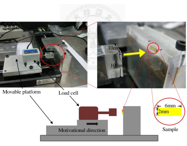
_R. As the system is unloading, the permanent deformation is obtained, and s is the _P permanent strain... 10 Figure 2–2. A schematic diagram of the Mooney-Rivlin model shows the dimension and principal stress t 、₁ t 、₂ t in ₃ X 、₁ X 、₂ X direction. ... 16 ₃ Figure 2–3. A schematic diagram of a linearly elastic model expresses extension in X ₂ direction of model when applied compression. ... 16 Figure 2–4. A schematic diagram of the dielectric elastomer model with a compliant electrode, shows the dimension, stretch and Maxwell stress ... 19 Figure 2–5. A schematic diagram of an electromechanical model. (a) No voltage drive (b) Applied a bias voltage. ... 22 Figure 2–6. The equilibrium point of electrostatic force and mechanical force [55]. ... 23 Figure 2–7. The relationship of normalized voltage and normalized thickness. ... 27 Figure 2–8. Dielectric elastomer electromechanical coupling system. (a) No voltage

(9)

applied on the sample. (b) Applied voltage ... 30 Figure 2–9. The capacitance experimental setup. (a) It is the experimental setup, using LCR meter (E498A) to measure capacitance of sample. (b) The electrodes of sample is separately clamped by clip. ... 32 Figure 2–10. Three type curves of stress and strain. (a) Single curvature. (b) One inflection point. (c) Two inflection point. The numbers of inflection point can determine the numbers of Mooney-Rivlin constant. ... 35 Figure 2–11. Mooney-Rivlin constant experimental setup. The figures above are separate photos of experimental setup and closed to sample. Below is the schematic figure of experimental setup. ... 35 Figure 2–12. Relationship of stress and strain with increases compression. ... 36 Figure 2–13. Normalized thickness vs. normalized voltage. This figure expresses pull-in effect of Mooney-Rivlin model. ... 38 Figure 2–14. A schematic diagram of the dielectric elastomer model with a compliant electrodes, shows that the current through the elastomer occurred between the compliant electrodes with applied voltage increases. ... 44 Figure 2–15. Normalize thickness vs. Normalize voltage. Shows that red line expresses as breakdown phenomenon and pull-in effect occur at the same time. In Ⅰ- region, slop of line is bigger than the slop of red line and expresses as breakdown phenomenon occurs before pull-in effect. Oppositely, slop of line is smaller than the slop of red line in Ⅱ- region and expresses as breakdown phenomenon occurs after pull-in effect. ... 44 Figure 3–1. Pre-strain stage setup. (a) Exploded view of pre-strain stage. (b) Schematic figure shows how to use the pre-strain stage. ... 47

(10)

Figure 3–3. Holding the sample VHB 4905 (10 mm10 mm0.5 mm) by pre-strain holder. It is no pre-strain. ... 49 Figure 3–4. Process of pre-strain. (a) Pre-strain= 200%, and maintain 2 hours. (c) Unscrew, and waiting for 2 hours. Sample almost backed to initial state, and the situation expresses that remnant stress is quite low. ... 50 Figure 3–5. Sputter coating machine (EMITECH K575X). ... 51 Figure 3–6. Sputter coating: gold (a) Positive side. (b) Opposite side. ... 52 Figure 3–7. (a) Sample stage is made of PMMA , and paste insulating tapes on stage. (b) To paste copper tapes to insulating tapes on both ends of stage. Coating Teflon which has low friction coefficient is helpful on experiment. (c) Schematic figure of sample stage. Size of stage is 50 mm20 mm5 mm, and the size of test sample is 6 mm2 mm0.5 mm. The copper tapes separately stick to compliant electrodes. ... 54 Figure 3–8. (a) Closed view of VHB 4905 actuator. (b) A optical image of the cross-section of VHB actuator. The surface electrodes are observed clearly.

The width of VHB is about 500 μm. ... 55 Figure 3–9. A schematic diagram of the whole experimental setup. The displacement of VHB actuator is measured by a laser displacement system (Keyence LK-G80). The USB high voltage generator (EMCO USB20P) applies DC voltage to the VHB sample by control of computer, and connects with the multimeter (Agilent 34410A). We can measure the electrical current by multimeter with series connection. ... 57 Figure 3–10. (a) A photograph of the experimental setup. (b) Test piece specification.

Notice that the displacement is measured at the center and the distance from the edge is 3mm. (c) A photograph of VHB actuator. ... 58

(11)

Figure 4–1. Displacement vs. Time and Current vs. Time. In upper figure, displacement increases with the increase of applied voltage. The minus sign of displacement indicates that the equivalent direction is compressive. When applied voltage increases to 2000 V, we observe sudden increasing current in lower figure. High current represents appearance of breakdown phenomenon. ... 61 Figure 4–2. Displacement vs. Voltage. The first sample is in experiment. With the increase of applied voltage from 0 V to 2000 V, displacement gradually becomes large. As applied voltage achieves 2000 V, breakdown phenomenon appears. The construction of this figure by compiles data from Figure 4–1. ... 62 Figure 4–3. Displacement vs. Voltage. The second sample is in experiment. With the increase of applied voltage from 0 V to 2000 V, displacement gradually becomes large. ... 62 Figure 4–4. Displacement vs. Voltage. The third sample is in experiment. With the increase of applied voltage from 0 V to 2000 V, displacement gradually becomes large. ... 63 Figure 4–5. Displacement vs. Voltage. The forth sample is in experiment. With the increase of applied voltage from 0 V to 2000 V, displacement gradually becomes large. ... 63 Figure 4–6. Displacement vs. Voltage, shows mean value of measurement and standard deviation. ... 65 Figure 4–7. Displacement vs. Voltage, shows mean value of measurement and standard

deviation. Red curve is the value of substituting experimental data to theory.65 Figure 4–8. Schematic figure of fringing electric field. ... 66

(12)

Figure 4–9. Normalized thickness vs. Voltage. With the increase of applied voltage from 0 V to 2000 V, displacement gradually becomes large. Figure illustrates that the result of experiment is close to theoretical value with decreases value of dielectric constant. When dielectric constant is 3.0, the result of experiment most fits theoretical value. ... 66 Figure 4–10. Normalized thickness vs. Normalized voltage, shows that red line expresses as breakdown phenomenon and pull-in effect occur at the same time. Green line is in Ⅰ- region, shoe that breakdown phenomenon occurs before pull-in effect due to experimental result. ... 69 Figure 4–11. Displacement vs. Voltage. The first test is in experiment. With the increase of applied voltage from 0 V to 1600 V, displacement gradually becomes large along upper path. Displacement gradually becomes small along lower path with the decrease of applied voltage from 1600 V to 0 V. The minus sign of displacement indicates that the equivalent direction is compressive.71 Figure 4–12. Displacement vs. Voltage. The second test is in experiment. With the

increase of applied voltage from 0 V to 1600 V, displacement gradually becomes large along upper path. Displacement gradually becomes small along lower path with the decrease of applied voltage from 1600 V to 0 V.

The minus sign of displacement indicates that the equivalent direction is compressive. ... 71 Figure 4–13. Displacement vs. Voltage. The third test is in experiment. With the increase of applied voltage from 0 V to 1600 V, displacement gradually becomes large along upper path. Displacement gradually becomes small along lower path with the decrease of applied voltage from 1600 V to 0 V.

The minus sign of displacement indicates that the equivalent direction is

(13)

compressive. ... 72 Figure 4–14. Displacement vs. Voltage. The forth test is in experiment. With the increase of applied voltage from 0 V to 1600 V, displacement gradually becomes large along upper path. Displacement gradually becomes small along lower path with the decrease of applied voltage from 1600 V to 0 V.

The minus sign of displacement indicates that the equivalent direction is compressive. ... 72 Figure 4–15. Displacement vs. Voltage, show mean value of measurement and error bar.

With the increase of applied voltage from 0 V to 1600 V, displacement gradually becomes large along upper path. Displacement gradually becomes small along lower path with the decrease of applied voltage from 1600 V to 0 V. The minus sign of displacement indicates that the equivalent direction is compressive. ... 74 Figure 4–16. Displacement vs. Voltage, shows mean value of measurement and error bar.

Red curve is the value of substituting experimental data to theory. ... 74

(14)

List of tables

Table 1-1. Summary of the advantages and disadvantages of the two major EAP groups

[9, 14, 20, 33]. ... 5

Table 2-1. Three different situations at equilibrium ... 25

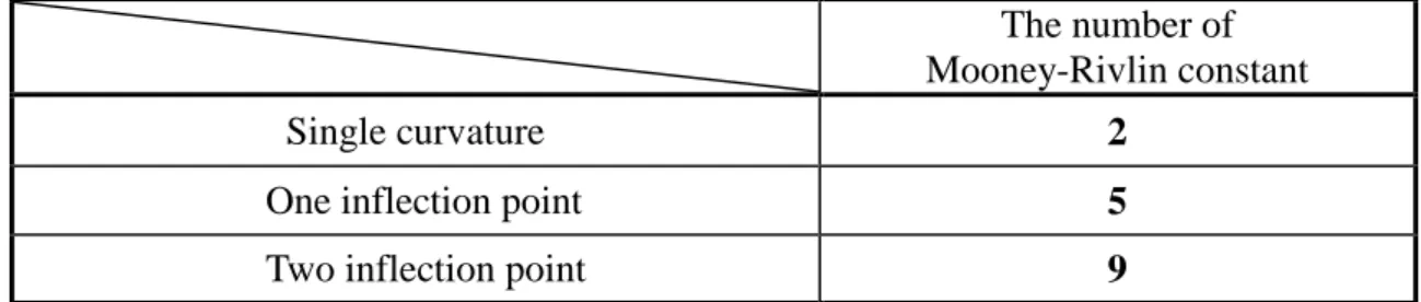
Table 2-2. The number of Mooney-Rivlin constant in three types. ... 33

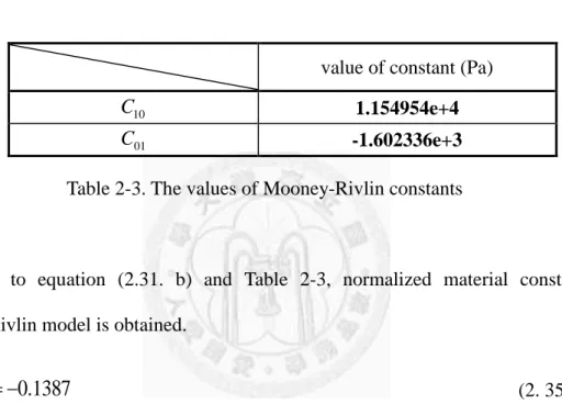
Table 2-3. The values of Mooney-Rivlin constants ... 34

(15)

List of symbols

V Applied voltage (V)

 Stress (MPa)

y Stress at yield point (MPa)

s Strain (%)

sy Strain at yield point (%)

sR Strain at breakdown point (%)

sP Permanent strain (%)

Y Young’s modulus (N/m²)

ti Principal(Cauchy) stress in X 、₁ X 、₂ X ₃ direction (MPa)

W Strain energy density function (J/ m³) C 10 Constant of Mooney-Rivlin model (Pa) C 01 Constant of Mooney-Rivlin model (Pa)

0

x i Initial length in X 、₁ X 、₂ X direction ₃ x i Final length in X 、₁ X₂ 、 X₃ direction

/ 0 i x xi i

  Normalized length in X 、₁ X 、₂ X direction ₃

V Normalized volume

1, 2

I I Strain invariants

0 Vacuum permittivity (F/m) = 8.85*10^-12(F/m)

r Dielectric constant (F/m)

 Poisson’s ratio (m³)

G Shear modulus (N/m²)

Pel Maxwell stress (N/m²)

C Capacitance of parallel-capacitor (F)

A Area of actuator cross thickness direction (mm²)

U Potential energy (J)

E Electric field (N/coul)

(16)

km Spring constant (N/m)

ke Equivalent spring constant of electricity (N/m) A 0 X - 1 X cross initial area of actuator (m₂ ²) g0 Initial gap between parallel-plates (m) g Displacement in thickness direction (m)

Fe Electrostatic force (N)

F m Mechanical force (N)

V P Pull-in voltage (V)

30 10/ 0

V

x C

^  Normalized voltage

01 10

C

 C Normalized material constant

A 0 X - 1 X cross initial area of actuator (m₂ ²) g0 Initial gap between parallel-plates (m) g Displacement in thickness direction (m)

10/ 0

e E

C 

 Normalized electric field

p Normalized voltage at pull-in

p Normalized thickness at pull-in

p p

p

e 

  Normalized electric field at pull-in

bd Normalized voltage at breakdown

bd Normalized thickness at breakdown

bd bd

bd

e 

  Normalized electric field at breakdown u e Energy density (J/ m³)

(17)

Chapter 1 Introduction

1.1 Background

Dielectric electroactive polymers (DEAPs) are materials for novel biomimetic actuators. They are composite materials consisting of film of dielectric polymer (such as silicones) and compliant electrodes. In comparison with other actuators (such as electromagnetic, piezoelectric [1] or shape memory ally [2] actuators) [3-8], attractive properties of DEAPs include large deformation, high speed of reaction, low cost, low elastic stiffness, high dielectric constant and relatively lightweight [9]. Therefore, they are suitable for medical and consuming applications [10]. In particular, DEAPs were shown to have better mechanical and electric performances [5, 8, 11-12]. Capabilities of DEAPs correspond to the performance of natural muscles, DEAPs actuators are often mentioned as artificial muscles [4, 8, 11, 13-16].

From 1999 to 2010, approximately 143 publications directly related to DEAPs have been published, including six books as summarized in Figure 1–1. It is noticed that there has been an obvious increase in the number of publications on DEAPs actuators over the last few years. In other words, the development of DEAPs has been getting considerable attentions recently. This result indicates that researchers have put their efforts on the analysis of working principle and applications about DEAPs which are important to us.

(18)

Figure 1–1. The histogram shows DEAPs publications from 1999 to 2010. The number of publications has increased over the last few years.

Year

Number of publications

Journal Conference Book

Histogram of DEAPs publications

(19)

1.2 Overview of Dielectric Electroactive Polymers 1.2.1 Brief history

Electroactive polymers (EAPs) have an alteration in shape which is applied by electric field. Their applications are mainly actuator and sensor. The researches of EAPs are traced back to 1880 when Roentgen observed alteration of length in a rubber-band by designed experiment of current test [4]. Then, in 1889, Secerdote proposed relative equation between strain and electric field by Roentgen’s experiment [14]. The breakthrough of research brought out the discovery of piezoelectric polymers in 1925.

However, due to relatively poor mechanical properties such as low strain and work output, main application is limited in sensors. In 1969, a material of DEAs, polyvinylidene fluoride (PVDF) which has large piezoelectric effect was proposed by Kawai et al. In 1980s, Millet and his coworkers presented the characteristics of polymer-metal composites. At the same time, electroactive polymers represented important conductive materials [17]. In the early 1990s, due to their attractive properties including large deformation and low driving voltage, ionic polymer-metal composites (IPMCs) are proposed [18-19].

There are various types of EAPs under investigation. Researchers mainly divided EAP materials into two groups, ionic and electronic EAPs as Figure 1–2 depend on their principle of operation [4, 9, 14]. Table 1-1 shows the summary of the advantages and disadvantages of the two major EAP groups. Our main objective of discussion is DEAPs.

DEAPs are composite materials consisting of film of dielectric polymer (such as silicones) and compliant electrodes. The dielectric polymers generally are sandwiched between two compliant electrodes. Electric force is generated by applied voltage which

(20)

squeezes the elastomer in the thickness direction and which cause the incompressible elastomer to expand in the area. In other words, they transform electric energy directly into mechanical work and produce large strain. First proposition for use as actuator by Pelrine et al. was proposed in 1998 [20]. Then, researchers proposed selection of DEAPs materials and analysis of their configurations [6, 21]. At the same time, the applications of DEAPs and development in technologies were also proposed [4, 22].

Moreover, simulation is also regarded as an important article in order to predict reliability and stability [23-26]. According to the statement above, directions of recent research are mainly applications, characteristics and simulating [27-32].

Figure 1–2. Classification of electroactive polymers [9].

(21)

EAP type Advantages Disadvantages

Electronic EAP

 Can operate in room conditions for a long time

 Rapid response (msec levels)

 Can hold strain under dc activation

 Induces relatively large actuation forces

 Large deformation

 Low cost

 Low elastic stiffness

 High dielectric constant

 Lightweight

 Requires high voltages (~150 MV/m). Recent development allowed for (~20 MV/m)

 Glass transition temperature is inadequate for low-temperature actuation tasks and, in the case of Ferroelectric EAP, high

temperature applications are limited by the Curie temperature.

 Due to associated electrostriction effect, a monopolar actuation is produced independent of the voltage polarity.

Ionic EAP

 large bending displacements

 Requires low voltage

 Natural bi-directional actuation that depends on the voltage polarity

 Except for CPs and NTs, ionic EAPs do not hold strain under dc voltage

 Slow response (fraction of a second)

 Bending EAPs induce a relatively low actuation force

 Except for CPs, it is difficult to produce a consistent material

 In aqueous systems, EAP suffer electrolysis at >1.23 V

 To operate in air requires attention to the electrolyte.

 Low electromechanical coupling efficiency.

Table 1-1. Summary of the advantages and disadvantages of the two major EAP groups [9, 14, 20, 33].

(22)

1.2.2 Working principle

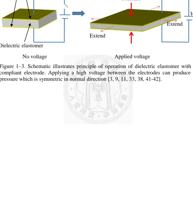
The dielectric polymers generally are sandwiched between two compliant electrodes and are regarded as the parallel-capacitor. The elastomers are almost incompressible but highly deformable. Applying a high voltage between the electrodes can produce a pressure which is symmetric in thickness direction, as shown in Figure 1–3. The pressure is called Maxwell stress [20, 32]. This pressure compresses DEA material between compliant electrodes and makes DEA material thinner; because of this, area of normal thickness is going to expand depending on incompressible volume.

Because of deformation, Cauchy stress is produced along the reverse thickness direction depending on a hyper-elastic model, Mooney-Rivlin model. Cauchy stress is produced by deformation so Cauchy stress also alters with applied voltage. Maxwell stress increases with applied voltage until Maxwell stress is equal to Cauchy stress. This situation is called force equilibrium. In the equilibrium point, we are going to discuss the pull-in effect [34-36] of electromechanical coupling system [30].

As electrostatic force equals to mechanical force, the electromechanical system is in equilibrium. For the discussion of system’s stability, considering three different situations at equilibrium, (i) stable, (ii) neutral stable, (iii) unstable. When gradient force is exactly equal to zero, the equilibrium situation is neutral stable. Neutral stable is a critical state between stable and unstable. Considering the physical meaning, the pull-in effect should occur in neutral stable. When pull-in effect occurs, the parallel electrodes should stick together.

In addition to pull-in effect, breakdown phenomenon [37-40] is also important.

With a high enough applied voltage, electrons can be freed from the atoms of dielectric elastomer, resulting in a high current through that material. The voltage is called breakdown voltage and the electric field is called breakdown electric field. Breakdown

(23)

phenomenon is going to make the properties of dielectric elastomer alter and destroy its structure. Thus, dielectric breakdown is an irreversible phenomenon. In chapter 2, we discuss these methods in-depth.

Figure 1–3. Schematic illustrates principle of operation of dielectric elastomer with a compliant electrode. Applying a high voltage between the electrodes can produce a pressure which is symmetric in normal direction [3, 9, 11, 33, 38, 41-42].

No voltage Applied voltage

Pressure

Extend

Extend V

Dielectric elastomer Complaint electrodes

(24)

1.3 Motivation and Purpose of research

In chapter 1.2.2, we simply introduce pull-in effect and breakdown phenomenon.

The DEA material exists between compliant electrodes, however, when pull-in effect occurs, the parallel electrodes should stick together. It is unreasonable due to incompressible property and mass conservation as it has the real material between compliant electrodes in our theoretical model. Because of this, if pull-in effect occurs in our model, it is unreasonable. If breakdown phenomenon occurs before pull-in effect, unreasonable situation does not occur. Because of this, we try to design our experiment and find the relationships of applied voltage, displacement, and current. Meanwhile, we derive the theory of the mechanical-electrical coupling model. Depending on theoretical and experimental results, we try to find which one occurs earlier.

The researches of reliability are important issues today. In our experiments, in addition to breakdown phenomenon, we also focus on reversibility [43]. Applied voltage which increases and decreases repeatedly act on DEA actuator and observe the alterations of displacement with time and increases applied voltage. Depending on this experiment, we can observe whether DEA actuator should be reversible or not.

In light of preceding concerns, this thesis has three purposes as follows: (a) to discuss breakdown phenomenon of DEA material which occurs before or after pull-in effect. (b) to discuss whether reversibility of DEA materials exist or not. (c) to propose a mechanical-electrical coupling model for predicting the deformation of DEAPs.

(25)

Chapter 2 Analytical model

2.1 Theory of elasticity 2.1.1 Introduction

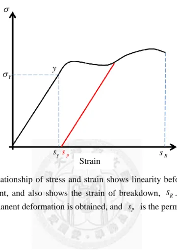
Usually, when considering a problem of general elastic material, we generally take only the linear part as the linear elastic material. Figure 2–1 can express the stress and strain on the relationship. With the increase of stress, we can observe the change of strain.

y expresses the yield point. Before strain reaches the yield strain,

s

_y, the stress is proportional to strain. The linear relationship of stress and strain [44] can be expressed as

= Ys

 (2. 1)

Where  is stress, s is strain, and Y is Young’s modulus.

According to Figure 2–1, it also illustrates the strain of breakdown,

s

_R. When reaching the breakdown point, the material behavior becomes unstable. The material cracks at the breakdown point. Because the behavior of materials alters over the yield point as the system is unloading, the relationship of stress and strain cannot maintain linearity. Because of the relationship of non-linearity, the permanent deformation is obtained, and s is the permanent strain. _P

For many materials, linear models do not accurately describe the observed material behavior. For example, the linear theory cannot be used in a rubber, which is a hyper-elastic material. Therefore, in the beginning of this chapter, we first briefly describe the theory of hyper-elastic materials and then discuss one of the hyper-elastic



(26)

models: Mooney-Rivlin model.

Figure 2–1. The relationship of stress and strain shows linearity before the strain does not reach yield point, and also shows the strain of breakdown,

s

_R. As the system is unloading, the permanent deformation is obtained, and s is the permanent strain. _P

s y

sy

Y

s R

s p

Strain

Stress



(27)

2.1.2 Hyper-elastic theory: Mooney-Rivlin model

In 18th century, James Bernoulli and Euler purposed the nonlinear elastic theory.

After they purposed the theory, Cauchy and Green were also separately purposed the elastic and hyper-elastic theory. The development is based on Green's theory which was simplified.

Hyper-elastic material’s relationship of stress-strain is derived from strain energy density function. When considering the hyper-elastic materials, we do not discuss Young's modulus, because Young's modulus alters with the strain and is not a constant value in this theory. Hyper-elastic theory not only provides a method of handling the material of this feature, but also constructs the physical model and describe its mechanical properties more easily.

Mooney-Rivlin model [45-46] is one of important hyper-elastic models.

Mooney-Rivlin model was obtained from the modified Neo-Hookean model. Scientists also identified the Neo-Hookean model as a special case of the Mooney-Rivlin model.

R. S. Rivlin et al [47]. proposed the general form of Mooney-Rivlin model:

2 2 2 2 2 2

2 1 2 3 2 1 2 3

1

[ _n( ⁿ ⁿ ⁿ 3) _n( ⁿ ⁿ ⁿ 3)]

n

W ^ A    B ^ ^ ^





       (2. 2)

Where W is the strain energy density function, A_2n and B_2n are the material constant of Mooney-Rivlin model, and ₁、₂、₃ are separately the normalized length in X 、₁ X 、₂ X direction: ₃

1 1

10

x

  x _{(2.2. a)}

2 2

20

x

  x _{(2.2. b)}

(28)

3 2

30

x

  x _{(2.2. c)}

Where x 、₁₀ x 、₂₀ x are separately the initial length, and ₃₀ x 、₁ x 、₂ x are separately ₃ the final length in X 、₁ X 、₂ X direction. ₃

According to equation (2. 2), we can take the first term for the equation as n1. Equation (2. 2) was simplified and rewritten as

2 2 2 2 2 2

10( 1 2 3 3) 01( 1 2 3 3)

W  C      C ^ ^ ^  (2. 3)

Where C₁₀ A₂ and C₀₁B₂ are the constants of the first order Mooney-Rivlin model, and determined from the experimental data.

Rivlin also argued that the strain energy must be a symmetrical even-powered function of the three principal stretches, and this kind of function can be expressed in terms of the strain invariants I and ₁ I which are defined below. ₂

2 2 2

1 1 2 3

I    (2.3. a)

2 2 2

2 1 2 3

I ^ ^ ^ (2.3. b)

Equation (2. 3) was rewritten as

10 1 01 2

( 3) ( 3)

W  C I   C I 

(2. 4)

Equation (2. 4) is the first form of Mooney-Rivlin model and is the common form to be used. Here we also propose several assumptions to facilitate the derivation: (i) incompressible volume (ii) isotropic (iii) uni-axial extension (compression). According to these assumptions, we can derive the above equations.

Due to Figure 2–2 and equation assumption (i) incompressible, V = constant , V is

(29)

volume of model.

1 2 3 = 1

   (2. 5)

And from assumption (ii) uni-axial extension (compression), we can assume that

3  and  ₁ ₂, we can rewrite equation (2. 5) as

1 2 3 1 1 3 1 2

3

1 1

1 ,

       

 

     (2. 6)

Substituting equation (2. 6) into (2. 3)

2

10 01 2

2 1

( 3) (2 3)

W C  C 

 

      (2. 7)

Cauchy stress is defined below.

i i

i

t  W p



  

 ^{(2. 8)}

Where

t

_i_and



_i are separately Cauchy stress and normalized length in X 、₁ X 、₂

X direction, 3 p is the hydration stress, W is the strain energy density function.

Substituting equation (2. 7) into (2. 8)

1 1

1

t  W p



  

 ^{(2.8. a)}

2 2

2

t  W p



  

 ^{(2.8. b)}

3 3

3

t  W p



  

 ^{(2.8. c)}

(2.8. c) - (2.8. b)

3 2 3 2

3 2

W W

t t  

 

 

  

  ^{(2.8. d)}

(30)

According to assumption (ii), and we can get the result:

t

₁

0  t

₂



Equation (2.8. d) can be rewritten as

2

3 10 01 2

2 2

( 2 ) (2 )

t  W C  C 

  

 

    

 (2. 9)

Equation (2. 9) can be expressed as the stress in

X

₃ direction from Figure 2–2, in that it is the normal stress in the Mooney-Rivlin model when considering a uni-axial stress.

When considering the stretch is tiny, equation (2. 9) can be expressed as below

3

10 2 01 3 10 01

1

2 4

lim t ( 4 ) (2 ) 6( )

Y C C C C

 

  



       

 (2. 9. a)

Where Y is Young’s modulus

As strain is relatively small, we can obtain the relationship of Young’s modulus and Mooney-Rivlin constant by equation (2. 9. a). We also consider the relationship of Young’s modulus and shear modulus, G.

2(1 )

G Y

 

 ^{(2. 9. b)}

In this equation,  is Poisson’s ratio, whose definition was expressed as

lateral axial

s

   s _{(2. 9. c)}

Where one strain s_lateral is in X or ₁ X direction, and another strain ₂ s_axial is in

X direction. 3 s_lateral and s_axial can be expressed as below due to Figure 2–3

2 20 20 2 20

20 20

( 1 1)

lateral

x x x x

s x x



 

    _{(2. 9. d)}

(31)

3 30 30 3 30

30 30

( 1)

axial

x x x x

s x x

 

 

    _{(2. 9. e)}

According to equation (2. 9. d) and (2. 9. e), equation (2. 9. c) can be rewritten as ( 1 1)

(1 )

( 1) = (1 )

 

   

 

   

(2. 9. f)

As the deformation is tiny, the value of Poisson’s ratio can be obtained by equation (2. 9. f).

1 1

(1 ) 1

lim lim

(1 ) 2

 

 

 

 

  

 (2. 9. g)

Substituting equation (2. 9. g) into (2. 9. b) according to equation (2. 9. a)

10 01

2( )

3

G  Y  C C (2. 9. h)

The above equation expresses the relationship of shear stress G and Mooney-Rivlin constant. R. S. Rivlin et al. proposed neo-hookean model, the model can be expressed as

2 2 2

1 2 3 1

( 3) ( 3)

2 2

hook

G G

W       I  (2. 9. i)

2 3,

( 2 2 )

hook 2

t G 



   (2. 9. j)

Where W_hook is the strain energy density of neo-hookean model. Comparison of equations (2. 9. i) and (2. 9. j) with (2. 7) and (2. 9), the result C₁₀G/ 2 can be obtained. According to equation (2. 9. h), we can find that neo-hookean model is a special case of Mooney-Rivlin model when C₀₁0.

(32)

energy density function. Hyper-elastic theory not only provides a method of handling the material of this feature, but also constructs the physical model and describe its mechanical properties more easily.

Figure 2–2. A schematic diagram of the Mooney-Rivlin model shows the dimension and principal stress t 、₁ t 、₂ t in ₃ X 、₁ X 、₂ X direction. ₃

Figure 2–3. A schematic diagram of a linearly elastic model expresses extension in X ₂ direction of model when applied compression.

X1

X3

X2

x3

x2

x30

x20

X1

X3

X2

t1

t2

 2

Principal stress

Compression

Extend Extend

(a) No compression (b) Compression

t3 Principal stress

(33)

2.2 Electromechanical analysis 2.2.1 Maxwell stress

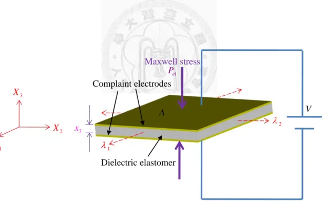
The dielectric polymers generally are sandwiched between two compliant electrodes and regarded as the parallel-capacitor. Applying a high voltage between the electrodes can produce a pressure which is symmetric in thickness direction (X ₃ direction), as show in Figure 2–4. The pressure is called Maxwell stress [6, 9, 20, 42, 48-49]. The derivation of Maxwell stress needs potential energy, U. The potential energy and capacitance of parallel-capacitor are separately defined as [50]

1 2

U  2 CV (2. 10)

0 3

r A

C x

   _{(2.10. a)}

Where C is the capacitance,



₀ is the vacuum permittivity (8.85  10^-12 C / N m ²  ² ),



r is dielectric constant, A is the area, V is the applied voltage between the electrodes, and

x

₃ is the thickness cross the compliant electrodes from Figure 2–3.

Substituting equation (2.10. a) to (2. 10)

0 2 3

1 2

rA

U V

x

   (2. 11)

According to incompressible volume, we can get the equation:

3 constant

V  A x  (2. 12)

In equation (2. 12), V is volume of model.

Equation (2. 12) (2. 12)can get the following equation by total differential.

(34)

3 3 0

dV  x dA  Adx  (2.12. a)

Equation (2.12. a) can be rewritten as

3 3

dx dA

x A

  _{(2.12. b)}

Potential energy U is also operated by total differential.

3 3

U U

dU dx dA

x A

 

 

  (2. 13)

Due to equation (2. 11) and (2.12. b), equation (2. 13) can be rewritten as

0 2 2 3 3

rA

dU V dx

x

   (2. 14)

The electrostatic pressure is defined as

3

1

el

P P dU

   A dx (2. 15)

According to equation (2. 14) and (2. 15), electrostatic stress, Maxwell stress, P is _el rewritten as

2 2 2

0 0 0

3 30

( ) ( )

el r r r

V V

P E

x x

     

       (2. 16)

In this equation, E is the electric field by applied voltage.The minus sign indicates that the equivalent pressure is compressive.

According to equation (2. 16), we can obtain the relationship of the variables.

Maxwell stress is proportional to square of the applied voltage and dielectric constant.

Maxwell stress is also inversely proportional to square of the depth across the electrodes.

As dielectric constant of material is larger and the applied voltage maintains constant, Maxwell stress increases with the value of dielectric constant, and vice versa. Similarly,

(35)

we hope that the applied voltage can be lower as Maxwell stress maintains constant.

From the statement above, a larger dielectric constant is necessary. Therefore, dielectric constant is an important factor of choosing the material. Maxwell stress is also affected by the geometric size of the model. If the thickness between compliant electrodes becomes thinner in the same Maxwell stress, applied voltage can be lower than the thicker thickness. In other words, Maxwell stress becomes larger in the same applied voltage. If Maxwell stress can be larger, the effect of compression is obvious, and it is good for us to establish the system of electromechanical coupling model. Depending on the statement above, thickness between compliant electrodes and dielectric are important factors for designing the experimental sample.

Figure 2–4. A schematic diagram of the dielectric elastomer model with a compliant electrode, shows the dimension, stretch and Maxwell stress

A

X1

X3

X2 x₃

 1

 2

Pel

V

Dielectric elastomer Complaint electrodes

Maxwell stress

(36)

2.2.2 Dielectric constant

TM TM

3M VHB 4905 which is chosen is an acrylic tape, and it has a higher dielectric constant [11-12, 41, 51-52]. Recently, the researches indicated deformation independent value of about 4.7 [12, 33, 41-42, 53]. This value was obtained by the capacitance experiment and the formula of parallel-capacitor with a dielectric [54].

0 3

r A

C x

   (2. 17)

In this equation, C is the capacitance,



₀ is the vacuum permittivity

(8.85  10^-12 C / N m ²  ² ),



_r is the dielectric constant, A is the area,

x

₃is the depth cross the compliant electrodes.

The capacitance C is obtained by the measurement of the capacitance. Area A and depth

x

₃ and the vacuum permittivity



₀ are known. Due to the statement above, we can obtain the dielectric constant



_r by equation (2. 17). The experiment of capacitance is going to be explained in chapter 2.4.1.

(37)

2.3 Construction of electromechanical model 2.3.1 Pull-in effect

Figure 2–5 is a schematic diagram of a parallel-capacitor which is supported by a mechanical spring whose force constant is k . Many electrostatic actuators typically _m include a deformable sheet which is supported by a mechanical spring. Mechanical spring is used to simulate dielectric layer between the electrodes. An important aim of this actuator is to achieve how much displacement the actuator does when applied to a bias voltage. We discuss this in Figure 2–5. First of all, we neglect the impact of gravity because the scale of an actuator is too small to affect it. When the bias voltage is applied between the electrodes, electrostatic force F can be expressed as below. _e

2 ' 2 '

2

0 0

( )

2( ) 2( )

e

V A V A

F U

g g g g

 

    

  (2. 18)

Where F is the electrostatic force, _e V is the applied voltage, g is the initial gap ₀ between the electrodes, g is the displacement in g direction, ^A^' is the area,  is the dielectric constant of dielectric layer between the electrodes.

According to equation (2. 18), electrostatic force, F increases with the decrease _e of compliant electrodes’ gap as applied a bias voltage between electrodes. Because of this, electrostatic force becomes obvious as the gap, and (g₀g) is very small.

The electrostatic force can also be expresses as an elastic spring system. We assume that F_e k g_e( ₀g), where k is the force constant of electricity. Equivalent _e spring constant of electricity can be expressed as the differential electrostatic force on the g direction. Due to equation (2. 18), we can obtain

(38)

2

3

( 0 )

e e

F V A

k g g g



  

  (2. 19)

Then the mechanical spring force can be expressed as

m m

F  k g (2. 20)

In equation (2. 20), mechanical force constant k does not alter with a small _m deformation.

Using the equation (2. 18) and (2. 20), we can obtain the Figure 2–6. In the Figure 2–6, one curve is the electrostatic force with alteration of the gap, another curve is the mechanical spring force with alteration of the gap. According to Figure 2–6, the relationship of mechanical spring force and alteration of the gap is linear, while the other one is not.

According to Figure 2–6, we can observe two points of intersection before reaching the equilibrium point. Although it has two points of intersection, two points are not both correct. Generally, the point of intersection closing the initial position is feasible.

Figure 2–5. A schematic diagram of an electromechanical model. (a) No voltage drive (b) Applied a bias voltage.

g0 k_m g

V Fe

Fm

g0g





(a) No voltage (b) Applied voltage

(39)

Figure 2–6. The equilibrium point of electrostatic force and mechanical force [55].

g0 g₀g F

3 2 1

Vp V V V

V1

V2

V3

Vp

Fe

Fm

Vp

V3

V2

V1

Increasing voltage

Critical point Initial position

(40)

As providing the particular applied voltage, the curve of electrostatic force and mechanical spring force intersect at tangent point to each other see Figure 2–6. This point shows that electrostatic force is equal to mechanical spring force and is canceled to each other. According to the point of intersection which is tangent point, the absolute values of gradient of two curves are the same. The particular voltage is called pull-in voltage, V_p. It is not stable state over pull-in voltage, in that the system is limited by pull-in voltage. According to equation (2. 19) and the statement above, the equation which was obtained can be expressed as

2

3

( 0 )

m e

k k V A

g g

  

 (2. 21)

Electrostatic force equals to mechanical spring force at the equilibrium point.

2

2( 0 )

e m m

F V A F k g

g g

   

 (2. 22)

Equation (2. 22) can be rewritten as

2 2 2k g g_m ( 0 g)

V A

  (2. 23)

Substituting equation (2. 23) to (2. 21), we can obtain the result.

0

1

g3g (2. 24)

According to equation (2. 24), the final gap between electrodes is one-third of the initial gap when the pull-in effect occurs. When substituting equation (2. 24) to (2. 23), we can obtain the pull-in voltage.

3

8 0

27

m p

V k g

A

 (2. 25)

We try to explain the pull-in effect by physical method. As electrostatic force is

(41)

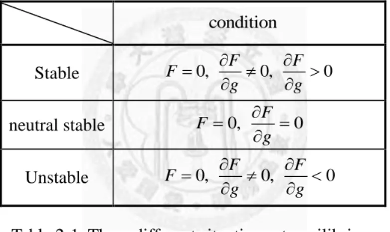
equal to mechanical spring force, the electromechanical system is in equilibrium. For the discussion of the system’s stability, we consider three different situations at equilibrium, (i) stable, (ii) neutral stable, (iii) unstable. When the condition is satisfied by gradient force which is greater than zero, the equilibrium situation is stable.

Oppositely, if gradient force is smaller than zero, the equilibrium situation is unstable.

When gradient force is exactly equal to zero, the equilibrium situation is neutral stable.

Neutral stable is a critical state between stable and unstable. We organize the statement into Table 2-1. Considering the physical meaning, the pull-in effect should occur in neutral stable.

Stable 0, F 0, F 0

F g g

 

  

 

neutral stable ^F ^0, ^F ⁰

g

  



Unstable ^F ^0, ^F ^0, ^F ⁰

g g

 

  

 

Table 2-1. Three different situations at equilibrium According to the statement above, we reconsider equation (2. 22)

2

2( 0 ) ^m

V A k g

g g

 _

 (2. 26)

Equation (2. 26) shows that the electrostatic force is equal to mechanical spring force.

Differential the force on g direction can be written as

2

3

( 0 ) ^m

V A k

g g

 _

 (2. 27)

Equation (2. 27) can be rewritten as

condition

(42)

3 2 2k g_m( 0 g)

V A

  (2. 28)

Substituting equation (2. 28) to (2. 27), we obtain the same result.

0

1 g3g

Substituting above equation to equation (2. 28), we also obtain the pull-in voltage.

3

8 0

27

m p

V k g

A



The equation (2. 26) can be dimensionless.

3

0 0 0

1-

2 _m

g g V

g g k g

A

 (2. 29)

Assuming x-y coordinate, x-axis is normalize voltage,

3

2 _m 0

V k g

A

, and y-axis is

normalize thickness,

0

g g ^.

We can see the figure in Figure 2–7.

In Figure 2–7, the red curve expresses that the sample is compressed with the applied voltage increases. This part is expectable. It reaches the critical point with the increasing voltage, and the pull-in effect should be observed at the point. At that time, the parallel sheets are going to stick together see Figure 2–6 and Figure 2–7. We are going to keep using the theory to derive the Mooney-Rivlin model.

(43)

Figure 2–7. The relationship of normalized voltage and normalized thickness.

Pull-in point

Normalized voltage

Normalized thickness

(44)

2.3.2 Elasticity and Maxwell stress combined

In Figure 2–8 (a), electromechanical coupling system is not driven. The initial depth across the compliant electrodes x is 0.5 mm, and the initial length ₃₀ x in ₁₀

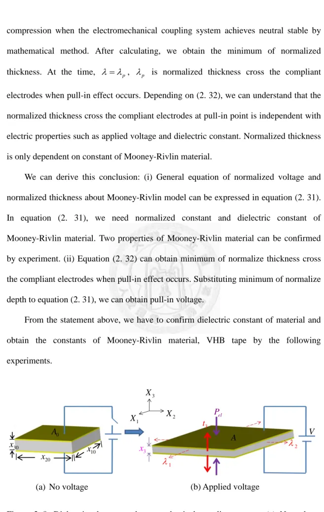
X direction is 2 mm, and the initial length 1 x in ₂₀ X direction is 6 mm. when ₂ applied voltage act on the system as Figure 2–8 (b), Maxwell stress is produced by applied voltage and gradually increases with applied voltage. At the same time, because of Maxwell stress is a compression, depth of dielectric elastomer across the compliant electrodes gradually becomes thinner. Because of incompressible volume, the depth is going to be compressed and the length expand in X and ₁ X direction when ₂ compression act on the system. Cauchy stress is produced by deformation. Because the deformation in direction of thickness comes from applied voltage, Cauchy stress also changes with applied voltage. Maxwell stress increases with applied voltage until Maxwell stress is equal to Cauchy stress. This situation is called force equilibrium. In the equilibrium point, we are going to discuss the pull-in effect of electromechanical coupling system.

Considering the physical meaning, the pull-in effect should occur at the point of force equilibrium, and three different situations at equilibrium, (i) stable, (ii) neutral stable, (iii) unstable. When gradient force is exactly equal to zero, the equilibrium situation is neutral stable. Neutral stable is a critical state between stable and unstable.

According to Table 2-1, we can obtain the conclusion in neutral stable. Equation (2. 9) and (2. 16) can be expressed as the equal by stress equilibrium from Figure 2–8. It can be written as below.

2 2

0 3 10 01 2

30

2 2

( ) ( 2 ) ( 2 )

el r

P V t C C

  x  

  

        (2. 30)

(45)

After applied voltage, deformation of material can be obtained. This deformation is the reason of producing Cauchy stress. Maxwell stress which is produced by applied voltage gradually increases until it is as large as Cauchy stress which increases by deformation of elastomer. When it is in force equilibrium, we can discuss the pull-in effect of Mooney-Rivlin model by Table 2-1. As Table 2-1, shows we can choose the state in neutral stable. In order to simplify the derivation, equation (2. 30) can be expressed as below by substituting dimensionless valuable.

2 2 3

(1 )( )

r

   

    (2. 31)

10 30

0

V x C







(2.31. a)

10 01

C

 C _{(2.31. b)}

Where  is normalized voltage, and



is normalized material constant of Mooney-Rivlin model. According to equation (2. 31), we need normalized material constant of Mooney-Rivlin model and dielectric constant in order to go the discussion about pull-in effect of Mooney-Rivlin. Because normalized material constant of Mooney-Rivlin model and dielectric constant are undetermined, two constants are separately obtained by experiments.

By differentiating on the normalized thickness  in X direction, the equation ₃ below can be derived from equation (2. 31).

3 2

4 3  1 0 (2. 32)

According to equation (2. 32), we also need normalized material constant of

介電致動高分子在崩潰電壓下與其材料可逆性的討論與研究

國立臺灣大學工學院機械工程學研究所 碩士論文

Department of Mechanical Engineering College of Engineering

National Taiwan University Master Thesis

介電致動高分子在崩潰電壓下與其材料可逆性的討論與研究 Dielectric Electroactive Polymers at Breakdown Voltage State and

Reversibility

張致國

Chih-Kuo Chang

指導教授：施文彬 博士 Advisor: Wen-Pin Shih, Ph.D.

中華民國 100 年 2 月

Feb, 2011

誌謝

摘要

Abstract

Contents

List of figures

s

List of tables

List of symbols

Chapter 1 Introduction

1.1 Background

1.2 Overview of Dielectric Electroactive Polymers 1.2.1 Brief history

1.2.2 Working principle

1.3 Motivation and Purpose of research

Chapter 2 Analytical model

2.1 Theory of elasticity 2.1.1 Introduction

s

s

s

2.1.2 Hyper-elastic theory: Mooney-Rivlin model



( 3) ( 3)

W  C I   C I 

t



t

0  t



X

2.2 Electromechanical analysis 2.2.1 Maxwell stress





x

2.2.2 Dielectric constant





x

x





2.3 Construction of electromechanical model 2.3.1 Pull-in effect

2.3.2 Elasticity and Maxwell stress combined



國立臺灣大學工學院機械工程學研究所碩士論文

指導教授：施文彬博士 Advisor: Wen-Pin Shih, Ph.D.