國立臺灣大學生命科學院生態學與演化生物學研究所 碩士論文
Institute of Ecology and Evolutionary Biology College of Life Science
National Taiwan University Master Thesis
臺灣西海岸中華白海豚族群之時空變異
Spatial Distribution and Temporal Variation of Indo-Pacific Humpback Dolphins (Sousa chinensis) in Western Taiwanese
Waters 郭毓璞 Yu-Pu Kuo
指導教授:周蓮香 博士
Advisor: Lien-Siang Chou, Ph.D.
誌謝
「不是最努力的一個,但絕對是最幸運的一個。」
這些年來,從一個茫然的二愣子到成一個能夠完成這篇論文在這裡寫謝辭的我,自知努 力程度絕對不足,小聰明也許有一點,但是最大的助力絕對是一路上遇到的各位貴人相助,
讓我的人生觀也在這碩班歷程中有所改變。
這篇論文的完成,首先要感謝這三年來一直相信我的潛力直到我在美國 SMM 大會開竅 後全力器重我的周蓮香教授,在架構上和用詞上幫我精雕細琢的郭秋雄老師,口試時給予我 諸多意見和鼓勵的邵廣昭、丁宗蘇、姚秋如三位老師,讓我學習到各種資料分析技能的李培 芬和謝志豪老師,更重要的是這些年來來自於漁業署、林務局、台電、台塑、國光石化等單 位的中華白海豚相關研究計畫讓我有資料可以分析,以及陪我行遍大江南北的楊留煜船長。
實驗室方面感謝分享了許多學術經驗和知識的大師兄祥麟,一路上犀利的鞭策著我的子 皓,在美國把我從深淵救回來上並總是花時間和我深談的欣怡,把 GIS 資料和技術交接給我 後仍經常好心回來幫忙的志慧,非常細心的建置了 Photo-ID 資料庫而且在最後幾個月被我遠 距諮詢了非常多次的維倫,在待人處世和關心社會上的榜樣明慶,在我茫然時給我很多幫助 和建議的陳瑩和惠雯,在口試預演時給我很多寶貴意見的 Anthony 和 Florence,當天幫我紀錄 和布置的羅婕與文達,幫助我處理很多行政事務讓我能專心在論文上的葉姊,在 PTT 上熱心 提供台大論文範本的阿德。出差方面則首先要感激海上的師父小章魚把我拉拔到獨當一面,
提供我許多生態攝影技巧和經驗的俊傑和昱閩,細心的忠斌,貼心的飛龍大哥,認真的象哥,
住過我心裡的思瑩,賦予我堅強和勇敢的蘇珊,給了我有益的人生歷練的圻鴻,接了我的班 的禹涵,提供並努力校正了無價資料的可愛妹妹侯雯,陪我一同到處下海的彥谷、張意等來 自各方的熱心志工們,一路上互相支援並一起闖入最終關卡的戰友彥頡與達勉,從資料分析 初期一路到最後的校閱都幫上大忙並給我無可取代的時光的 Peggy,幫我整理過資料或幫忙出 差收資料的家欣、彥樺、純如、凱盈、欣樺、幸娜等學生和志工們,有如我另一個家的協會 的雪倩、楊姊和淑紋姊和志工們,讓我能在走之前有幸帶到的貞儀。
友人方面則感謝在碩一甩了我讓我從中二畢業進化成孤僻而從此心無旁騖的小吳、最惹 我厭又讓人無法拒絕的孽緣仕翰、紅顏知己珮綺、小秉和梵弦、陪我耍廢耍憤青的潛之、宅
中文摘要
中華白海豚(Sousa chinesis)主要分布在印度東岸至澳洲東部的近岸淺水區 域,其中分布在臺灣西海岸的族群被認為是數量稀少且獨立封閉的族群,且在 IUCN 紅皮書上被列為「極度瀕危」等級。本研究採用海上穿越線調查法以及「標記-再 捕捉」法進行該族群豐度之估算,並分析其空間分佈和族群動態。穿越線設計方 面,除了 2008 年到 2012 年共執行 394 天趟的傳統平行海岸穿越線調查外,本研 究在 2012 年至 2013 年期間另外執行 26 天趟的 Z 字型穿越線調查以擴大調查範圍,
橫跨海豚所有可能棲地,最後進行兩種方式之比較。此外,就過去五年研究所累 積之 75 隻非嬰幼個體照片資料庫,採用標記-再捕法的「穩健設計模式」來估算 歷年族群豐度、死亡率、出生率之變化。海上調查 Z 字型穿越線的結果顯示中華 白海豚呈現近岸淺水分佈,出現於平均水深 7.9±0.79 (SE)公尺的水域,有些河 口偏好傾向,且其可能棲地範圍可能超出本調查之南北界。族群密度方面,相對 於 Z 字型調查估算結果為 0.103 隻/平方公里 (CV=42.0%),平行海岸線則為 0.31 隻/平方公里 (CV=11.5%);豐度估算方面,兩方法的結果則相當接近,分別為 64 隻 (95%CI: 29-144)或 68 隻 (95%CI: 54-85),因此就這個近岸淺水分布的小族 群,近岸平行海岸線可以視為一種合適的穿越線設計。族群的近五年間動態分析 方面,結果首度明確顯示族群數量從 2010 年的 75 隻下降到 2012 年的 64 隻,還 伴隨下滑的族群存活率和出生率,尤其是粗出生率從 2009 年的 7.14%到 2012 年急 遽下降至零。針對臺灣狀況如此危急的小族群,在區域性滅絕之前,急需針對此 警訊深入研究起因,並展開有效的保育行動。
關鍵字:中華白海豚、穿越線調查、標記-再捕捉法、分布、族群動態、保育
ABSTRACT
Indo-pacific humpback dolphins (Sousa chinensis, a.k.a. Chinese white dolphins), are widely distributed in inshore shallow waters between eastern India and Australia.
The population off the western coast of Taiwan is considered to be a small isolated population, categorized as “Critically Endangered” in the IUCN red list. The purpose of this thesis is to estimate the abundance of this population by two commonly used methods, the transect line survey and mark-recapture method, and to investigate the dolphins’ spatial distribution and population dynamics. Two designs of transect line surveys were used-- 394-day inshore parallel transect line surveys conducted between 2008 and 2012, and 26-day zigzag transect line survey was conducted between 2012 and 2013 that covered the whole possible habitat of this dolphin species, and their results were compared later. In addition, based on the photo-ID data assembled over the past 5 years’ researches that consisted of 75 identified individuals, a robust design mark-recapture method was used to estimate the yearly changes in abundance, as well as mortality and the crude birth rate. The results of zigzag transect lines confirmed that the Chinese white dolphins were concentrated in inshore shallow waters, with average water depths at 7.9±0.79(SE) m, showing some indication of preference for estuarine environments, while their potential habitat range could extend further north and south than previously assumed. The population density was estimated by the zigzag survey as
distribution of the Chinese white dolphins in Taiwan is limited to inshore shallow waters, the inshore parallel surveys could serve as an effective and valuable transect line design for density and abundance studies on this population. In addition, the analysis of the robust design mark-recapture model showed a significant declining trend in the dolphin’s population, with the annual abundance dropping from 75 individuals in 2010 to 64 individuals in 2012, while the survival and birth rates decreased. In particular, the present study revealed for the first time the dramatic drop of the animal’s crude birth rate from 7.14% in 2009 to zero in 2012. For a population as small as the one in Taiwan, this finding requires special attention, and further researches and effective conservation actions must be taken place soon before the Chinese white dolphin population in Taiwan becomes regionally extinct.
Keywords: Chinese white dolphins (Sousa chinensis), transect line, mark-recapture, distribution, population trend, conservation
CONTENTS
誌謝 ...i
中文摘要 ... ii
ABSTRACT ... iii
CONTENTS ... v
LIST OF FIGURES ... viii
LIST OF TABLES ... x
Chapter 1 General Introduction ... 1
1.1 Indo-pacific Humpback Dolphins... 1
1.2 Distribution and Habitat Preference ... 1
1.3 Anthropogenic Threats ... 3
1.4 Methods for Abundance Estimation ... 3
1.4.1 Transect line survey ... 4
1.4.2 Mark-recapture method ... 5
1.5 Worldwide Abundance Studies on Indo-Pacific Humpback Dolphins ... 6
1.6 Population Status in Taiwan Western Waters ... 7
1.7 Objectives of this study ... 8
References ... 10 Chapter 2 Population density and abundance estimation of Chinese white dolphins (Sousa chinensis) in the western coastal waters of
2.2.2 Survey Operation ... 25
2.2.3 Zigzag Transect Line Survey ... 26
2.2.4 Environmental Factors ... 27
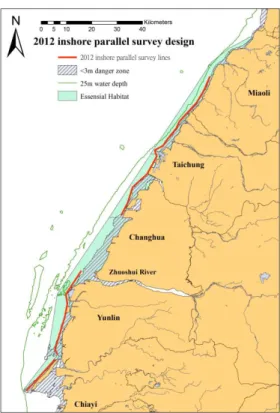
2.2.5 Inshore Parallel Transect Line Survey ... 27
2.2.6 Distance Sampling ... 28
2.2.7 Comparison among Nearby Populations ... 30
2.3 Results ... 31
2.3.1 Spatial Distribution ... 31
2.3.2 Density and Abundance Estimates from Zigzag Transect Lines ... 31
2.3.3 Environmental Factors ... 32
2.3.4 Density and Abundance Estimates from Inshore Parallel Transect Lines ... 33
2.3.5 Comparison with Studies on Nearby Populations ... 34
2.4 Discussion ... 35
2.4.1 General Distribution from the Zigzag Survey ... 35
2.4.2 Habitat Preference in the Study Area ... 36
2.4.3 Transect Line Assumptions ... 38
2.4.4 Density and Abundance Estimates ... 38
2.4.5 Annual Variation of Inshore Parallel Transect Estimates ... 41
2.4.6 Conservation Status and Implication ... 42
References ... 43
Chapter 3 Population trend of Chinese white dolphins (Sousa chinensis) in the western coastal waters of Taiwan-by mark-recapture method ... 66
3.1 Introduction... 68
3.2 Material and methods ... 72
3.2.1 Data Collection ... 72
3.2.2 The Robust Design Mark-recapture Method ... 73
3.2.3 Unmarked Ratio (𝜃) ... 74
3.2.4 Crude Birth Rate ... 75
3.2.5 Spatial and Temporal Variations in Population Estimates ... 76
3.3 Results ... 77
3.3.1 Data Description ... 77
3.3.2 Model Selection and Parameter Estimates ... 77
3.3.3 Unmarked Ratio and Corrected Population Size ... 78
3.3.4 Crude Birth Rate ... 79
3.3.5 Spatial and Temporal Variations in Population Estimates ... 79
3.4 Discussion ... 81
3.4.1 Mark-recapture Assumptions ... 81
3.4.2 Parameter Estimates ... 82
3.4.3 Variations in Reproductive Indicators ... 83
3.4.4 Spatial and Temporal Variations in Population Estimates ... 84
3.4.5 Conservation Implications ... 86
References ... 88
Chapter 4 Conclusion ... 98
LIST OF FIGURES
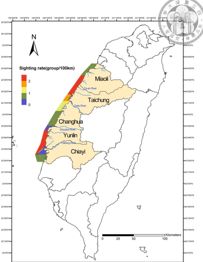
Fig. 1.1 Sighting rate of Chinese white dolphins in different areas off western
Taiwan waters (Chou 2011) ... 17
Fig. 1.2 Framework of this study ... 18
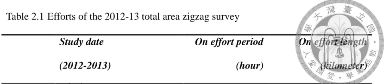
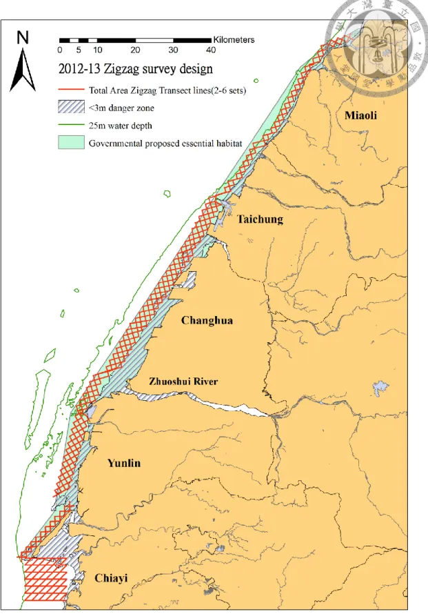
Fig. 2.1 Total area zigzag survey design in 2012-2013 ... 51
Fig. 2.3 Zigzag survey design’s defined study area in 2012-2013 ... 52
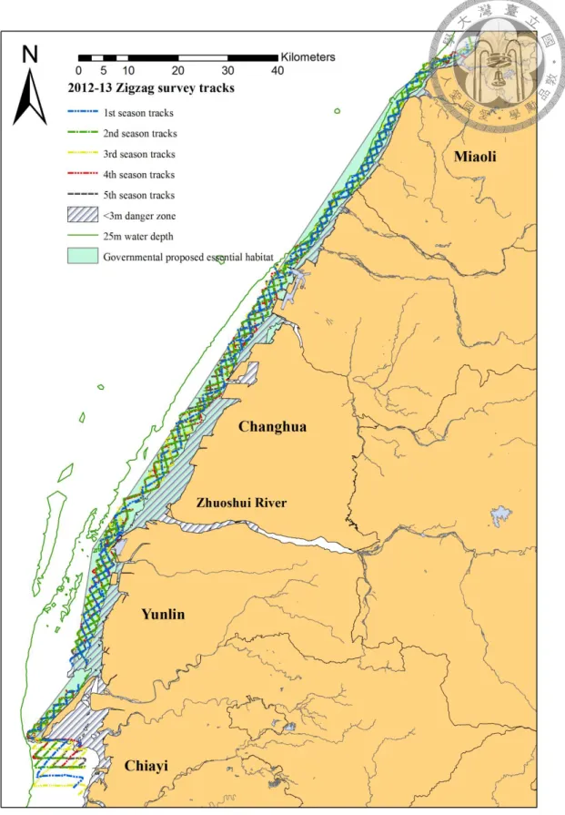
Fig. 2.4 Zigzag survey tracks of the five survey seasons in 2012-2013 ... 53
Fig. 2.5 Sighting points (n=23) of the five survey seasons in 2012-2013 ... 54
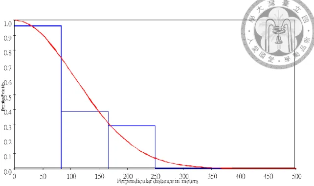
Fig. 2.6 Best fit model’s detection probability function (curve) and observed perpendicular distances (histogram) of the total area zigzag survey. ... 55
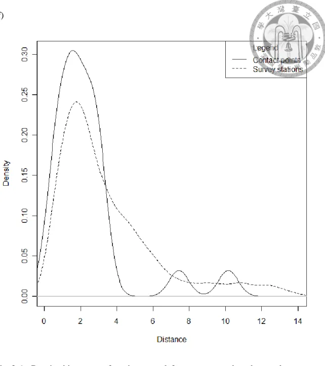
Fig. 2.7 Density histogram of environmental factors measured at the regular survey stations (dotted line) and at the contact points (solid line) during the 2012-13 zigzag survey: (a) Salinity (ppt), (b) Temperature (°C), (c) Water depth (m), (d) pH value, and (e) Turbidity (NTU) (f) Distance to shore (km)61 Fig. 2.8 Transect line design for inshore parallel surveys in (a) 2008, (b) 2009, (c) 2010, (d) 2011 and (e) 2012. ... 63
Fig. 2.9 Study area covered by inshore parallel surveys ... 64
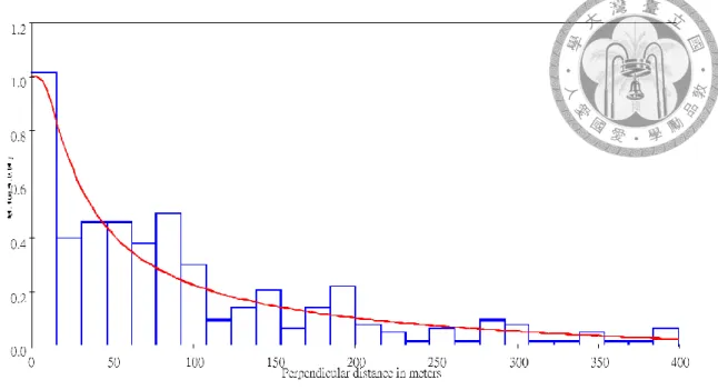
Fig. 2.10 Best fit model’s detection probability function (curve) and observed perpendicular distances (histogram) of the 2008-2012 inshore parallel survey. ... 65
Fig. 3.1 Monthly variation in survey trips between 2008 and 2012 ... 95
Fig. 3.2 Frequency distribution of various dolphin group sizes. ... 95 Fig. 3.3 Discovery curve of the Chinese white dolphins in Taiwan between 2007 and
2012 ... 96 Fig. 3.4 Frequency distribution of sighting rates of the 75 identified individuals of Chinese white dolphins in Taiwan ... 96 Fig. 3.5 Annual changes in dolphin population abundance with mean and 95%
confidence interval... 97
LIST OF TABLES
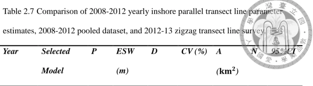
Table 1.1 Abundance estimates of Indian humpback dolphins (Sousa plumbea) worldwide ... 15 Table 1.2 Abundance estimates of Chinese white dolphins (Sousa chinensis) worldwide ... 16 Table 2.1 Efforts of the 2012-13 total area zigzag survey ... 46 Table 2.2 Parameter estimates of the zigzag transect line surveys ... 46 Table 2.3 Descriptive statistics of environmental factors measured from the survey stations of zigzag transect line surveys ... 47 Table 2.4 Descriptive statistics of environmental factors measured from the dolphin contact points of zigzag transect line surveys... 47 Table 2.5 Effort and study area of the 2008-12 inshore parallel survey ... 48 Table 2.6 Parameter estimates of the 2008-12 inshore parallel transect line surveys .. 48 Table 2.7 Comparison of 2008-2012 yearly inshore parallel transect line parameter estimates, 2008-2012 pooled dataset, and 2012-13 zigzag transect line survey. ... 49 Table 2.8 Comparison of density and abundance estimations of Chinese white dolphins in Chinese and Taiwanese waters... 50 Table 3.1 Results of the first six best models in robust design mark-recapture ... 91 Table 3.2 Annual estimates of abundance and other parameters based on the best model ... 91 Table 3.3 Annual estimates of abundance and other parameters based on the second best model with survivorship varying with time “S(t)” ... 92
Table 3.4 Annual crude birth rate (CBR) of the Chinese white dolphins in Taiwan .... 92 Table 3.5 Population abundances of the Chinese white dolphins in South China Seas estimated by the mark-recapture method ... 93 Table 3.6 Yearly estimates of population abundance of the Chinese white dolphins in Taiwan ... 94
Chapter 1 General Introduction
1.1 Indo-pacific Humpback Dolphins
Indo-Pacific humpback dolphins (also known as Chinese white dolphins, Sousa chinensis, Osbeck 1765) are widely distributed from African to Australian waters, and generally inhabit shallow waters near the shore with water depth less than 20 meters (Jefferson and Karczmarski 2001).
The taxonomy of Indo-Pacific humpback dolphins is still unsettled with little known information on genetics. Most taxonomists now consider the Indo-Pacific humpback dolphins to consist of two species by their geographical distribution: Indian humpback dolphins (Sousa plumbea, Cuvier 1829) from South Africa to the eastern coast of western Indian waters, and Chinese white dolphins (Sousa chinensis, Osbeck 1765) from eastern Indian waters to Australian waters (Jefferson and Van Waerebeek 2004). This two-species classification was adopted by the IUCN (Reeves et al. 2012).
However, recent mitochondrial DNA (mtDNA) studies showed that the Australian humpback dolphins are very different from these two species, indicating a unique evolutionary clade (Frère et al. 2008; Lin et al. 2010). Therefore, there remains some space for the discussion of their taxonomic status.
1.2 Distribution and Habitat Preference
Indo-Pacific humpback dolphins are mainly distributed in very shallow and inshore waters worldwide (Chen et al. 2008; Jefferson 2000; Karczmarski et al. 2000; Parra et al. 2004; Wang et al. 2004; Yeh 2011), with water depths no greater than 30 m (Atkins et al. 2004; Hung 2008; Parra et al. 2006; Wang et al. 2007). Water depth is considered
to be the key environmental factor limiting their distribution. In South Africa, Karczmarski et al. in 2000 proposed the 25 m isobaths as the critical water depth of the dolphin’s occurrence, and that the presence of dolphins was concentrated mainly at water depths less than 15m (Karczmarski et al. 2000; Parra 2006). In Hong Kong, the dolphins showed significant preference for steep benthic slopes (Hung 2008). In Taiwan, the maximum and standard deviation of water depth were known to be the key factors in habitat preference (Yeh 2011).
In addition, preferences at estuaries, harbor mouths, and even dredge channels were also reported (Atkins et al. 2004; Chen et al. 2009; Jefferson and Hung 2004;
Parra 2006; Parra et al. 2006). The preference was claimed to be associated with the dolphin’s feeding behavior (Hung 2008; Parra 2006) on estuarine-associated fish such as benthic croakers and epipelagic anchovies, cutlass fish, sardines, and mullets (Jefferson 2000; Barros et al. 2004). In Algoa Bay, South Africa, dense area use and feeding activities in rocky reefs provided another habitat preference clue (Karczmarski et al. 2000).
Regarding hydrological factors, surface temperature, salinity, and turbidity were commonly tested, but results were not consistent. In Hong Kong, the dolphin density was negatively correlated with sea surface temperature, salinity, and turbidity (Hung 2008). Similarly, around Brother’s Island, Hong Kong, the dolphin sighting rate was negatively correlated with salinity (Jefferson 2000). In Algoa Bay, it was reported that the distribution and group size of Chinese white dolphins fluctuated with sea surface
distribution (Hung 2008). Notably, all of these preferences for hydrological factors were considered to be indirect indicators of prey distribution, rather than the dolphins themselves (Karczmarski et al. 1999; Hung 2008).
1.3 Anthropogenic Threats
Because of the limited to inshore distribution, Chinese white dolphin populations face extensive anthropogenic disturbances (Jefferson et al. 2009;
Karczmarski et al. 1998; Ross et al. 2010). These anthropogenic threats could have direct or indirect impacts on Chinese white dolphins. Direct threats such as incidental catches, accidental bycatches, and vessel collisions from fisheries could cause injury or mortality in the population. Near shore industrial development will cause habitat degradation, pollution from sewage discharge, and noise, all of which will change the animal’s habitat preference, physiological and behavioral responses. And for indirect threats, which were mainly on prey competition among fisheries and dolphins, could cause long-term population sustainability problems.
1.4 Methods for Abundance Estimation
In population ecology, abundance estimation is an important task for understanding the species as well as its conservation status for management. In ecological field surveys, there are many standard ways to estimate abundance, e.g. territory mapping, drive count, point count, transect line, capture method, removal method, and mark-recapture method (Lancia et al. 1994).
In marine mammal research, transect line and mark-recapture methods are the two main ways that have been commonly adopted because of operational convenience. The transect line method estimates the abundance in an area, and the mark-recapture method estimates the abundance of the population itself. These methods have been widely applied in cetacean surveys around the world (Transect lines: Forcada and Hammond 1998; Kreb 2002; Slooten et al. 2006; Vidal et al. 1997; Mark-recapture: Gormley et al.
2005; Stensland et al. 2006; Wilson et al. 1999).
1.4.1 Transect line survey
The transect line survey is one type of distance-based sampling method (Buckland et al. 2005). In distance sampling, point count and transect line are two basic approaches, where the point count is suitable for clustered animals like in bird studies (Ralph et al. 1998), and transect line is often applied on ranging animals, especially marine mammals (Burnham et al. 1980). A standard transect line survey should systematically sample a specific study area by many straight lines, and counts the size of every sighted group, measuring the perpendicular distance from the transect lines to fit a detection probability model, so that the density can be estimated (Buckland et al.
1993).
When applying this kind of survey, there are some basic transect line assumptions that need to be considered: (1) Objects directly on the line or point are detected with
transect data and other environmental data such as weather, waves, ship types, and observers, Barlow et al. 2001 concluded that most of these factors could affect the ESW, which is worth considering when applying this survey method.
1.4.2 Mark-recapture method
The mark-recapture method can estimate the abundance itself, and can further investigate the reproductive (survival rate) and migratory (immigration/emigration rate) parameters. Traditionally, this method consists of three steps: capture, mark, and recapture. First, traps and nets are used to capture some individuals in the population. Then, by applying tags, collars, clipping, or bands on captured animals, these animals are marked and can be recognized later.
If the capture and recapture probabilities in subsequent capture processes are the same, then by calculating the proportion of marked individuals in the recapture group with respect to the number of marked individuals in the capture group, the population size can be easily estimated by this classic Lincoln-Peterson method (Amstrup et al. 2010).
To apply this method, some assumptions must be met: (1) All marks are unique. (2) Marks cannot change or be lost. (3) Marks are recognizable and correctly recorded and reported. (4) All animals in the population have the same probability of being captured. (5) The animals can survive and show no negative effects after the marking process. (6) The population is closed to births, deaths, immigration and emigration (for closed population models).
This classic formula can only work on idealistic closed populations with no population changes over the study period. But in most scenarios, the population is open and fluctuates with survivorship and mortality or migration from other subpopulations. Some modified models have been designed to address this problem, such as the Cormack and Jolly-Seber models for open populations (Nichols 1992).
Because the physical marking processes mentioned above would inevitably affect or hurt the animals, a passive capture and mark method, photo -identification, based on photo shooting and recognition of the natural markings of the animal is recommended in mark-recapture research, especially on small cetaceans (Würsig and Jefferson 1990; Hammond et al. 1990).
1.5 Worldwide Abundance Studies on Indo-Pacific Humpback Dolphins
Across the entire distribution area of Indo-Pacific humpback dolphins, many research teams have applied either the transect line survey or mark-recapture method to estimate the regional abundance of the populations. Table 1.1 and Table 1.2 summarize the worldwide abundance estimates with the method applied and 95%CI. As shown,
less than 300 individuals, as quite low for small cetaceans.
1.6 Population Status in Taiwan Western Waters
In Taiwan, Indo-Pacific humpback dolphins (hereafter Chinese white dolphins) are widely distributed in the shallow waters along the western Taiwanese coast (Yeh 2011) and are believed to be isolated from populations in adjacent waters such as Xiamen and Hong Kong (Wang et al. 2008). The very first studies on Chinese white dolphins by Wang et al. (2004, 2007) indicated that Chinese white dolphins were distributed across the inshore waters from Tongxiao (通宵) to Taixi (台西), along approximately 100 km of coastline, and that the dolphins occurred within about 2 km from the shore.
According to studies conducted by Lien-Siang Chou in recent years, not only the habitat range was expanded to Longfong (龍鳳) harbor of Miaoli (苗栗) County to Jiangjun (將軍) harbor of Tainan (台南) County, but also reported that there were two “hotspots”
with high sighting rates, from Baishatun (白沙屯) to the Changbin Industrial Park (彰濱 工業區), and from Liuqing Industrial Park (六輕工業區) to the Waisanding Sandbar (外傘頂洲) (Fig. 1.1, Chou 2011; Yeh 2011).
The abundance of this population has been estimated by various studies. It was first estimated to consist of 99 individuals (CV=51.6%) by Wang et al. (2007) using the transect line survey method, and in 2012 was estimated to be 74 individuals (CV=4%) by the mark-recapture method. Lien-Siang Chou’s team has further identified a great majority of the members in this population based on the dolphins’ photo data, including 71 identified individuals and 27 calves born between 2006 and 2010 (Chang 2011), and estimated the abundance to be 75 individuals by the mark-recapture method (Yu et al.
2010). Overall, the Taiwanese population should be closed and contained less than 80
individuals. The conservation status of this special regional population is so critical that it was listed in the IUCN Red List of Threatened Species as “critically endangered”
(Reeves et al. 2008).
After a recent study conducted by Lien-Siang Chou’s team, most of the individuals (excluding calves) in Taiwan’s dolphins population were identified, and social interactions and reproductive parameters were estimated (Chang 2011). In addition, an ecological modeling study has marked out some influential environmental factors: water depth, salinity and distance to shore (Yeh 2011), that may affect the Chinese white dolphins’ distribution, which was also supported by the study in South Africa (Karczmarski et al. 2000). Ko's study (2011) showed significant overlapping between fishery intensity and Chinese white dolphins’ presence. Nevertheless, heavy scar rates from both anthropogenic (42%) and natural (25.4%) threats implied a significant impacts on the population (Lin 2012).
For conservation management on this small population, an “essential habitat” of Chinese white dolphins with 763 𝑘𝑚2 was proposed by the Forestry Bureau off the western coast of Taiwan in the year of 2011 (Shao and Chou 2012). Considering management on such a large protect area, a specific approach for the detailed information on habitat ranging, spatial distribution and abundance estimates will be very critical for further researches and practical conservation acts design, and may benefit to the sustainability of this small and vulnerable population.
estimate the abundance of Chinese white dolphins in Taiwan (Fig. 1.2). A newly designed zigzag transect line survey was deployed across the whole possible habitat range. Besides the analysis on their spatial distribution and habitat preferences, population density and abundance were estimated based on the data collected from zigzag survey from 2012 to 2013 as well as previous inshore parallel surveys between 2008 and 2012. Regarding the mark-recapture method, by applying robust design model, abundance and some reproductive parameters were estimated by each year to determine the population trend. Finally, I hope to find a good method for long-term monitoring program of this local population after comparing various estimation methods.
References
Amstrup, Steven C, Trent L McDonald, and Bryan FJ Manly. 2010. Handbook of Capture-recapture Analysis. Princeton University Press.
Atkins, Shanan, Neville Pillay, and Victor M Peddemors. 2004. “Spatial Distribution of Indo-Pacific Humpback Dolphins (Sousa chinensis) at Richards Bay, South Africa: Environmental Influences and Behavioural Patterns.” Aquatic Mammals 30 (1): 84–93.
Barlow, Jay, T Gerodette, and Jaume Forcada. 2001. “Factors Affecting Perpendicular Sighting Distances on Shipboard Line-transect Surveys for Cetaceans.” Journal of Cetacean Research and Management 3 (2): 201–212.
Barros, Nélio B, Thomas A Jefferson, and ECM Parsons. 2004. “Feeding Habits of Indo-Pacific Humpback Dolphins (Sousa chinensis) Stranded in Hong Kong.”
Aquatic Mammals 30 (1): 179–188.
Buckland, S. T., D. R. Anderson, K. P. Burnham, and J. L. Laake. 1993. Distance Sampling: Estimating Abundance of Biological Populations. London: Chapman
& Hall.
Buckland, Stephen T., David R. Anderson, Kenneth P. Burnham, and Jeffrey L. Laake.
2005. “Distance Sampling.” In Encyclopedia of Biostatistics.John Wiley & Sons, Ltd..
Burnham, Kenneth P., David R. Anderson, and Jeffrey L. Laake. 1980. “Estimation of Density from Line Transect Sampling of Biological Populations.” Wildlife Monographs (72) (April 1): 3–202. doi:10.2307/3830641.
Cagnazzi, Daniele De Biasi, Peter L. Harrison, Graham J. B. Ross, and Peter Lynch.
2011. “Abundance and Site Fidelity of Indo-Pacific Humpback Dolphins in the Great Sandy Strait, Queensland, Australia.” Marine Mammal Science 27 (2):
255–281. doi:10.1111/j.1748-7692.2009.00296.x.
Chang, W. L. 2011. “Social Structure and Reproductive Parameters of Indo-Pacific Humpback Dolphins (Sousa chinensis) Off the West Coast of Taiwan.” Master thesis, National Taiwan University.
Chen, Bingyao, Dongmei Zheng, Guang Yang, Xinrong Xu, and Kaiya Zhou. 2009.
“Distribution and Conservation of the Indo–Pacific Humpback Dolphin in China.” Integrative Zoology 4 (2): 240–247.
doi:10.1111/j.1749-4877.2009.00160.x.
Chen, Bingyao, Dongmei Zheng, Feifei Zhai, X. Xu, P. Sun, Q. Wang, and G. Yang.
2008. “Abundance, Distribution and Conservation of Chinese White Dolphins (Sousa chinensis) in Xiamen, China.” Mammalian Biology – Zeitschrift Für Säugetierkunde 73 (2) (March 15): 156–164.
doi:10.1016/j.mambio.2006.12.002.
Chen, Tao, Samuel K. Hung, Yongsong Qiu, Xiaoping Jia, and Thomas A. Jefferson.
Asian Marine Biology 14: 49–59.
Durham, Ben. 1994. “The Distribution and Abundance of the Humpback Dolphin (Sousa chinensis) Along the Natal Coast, South Africa”. University of Natal.
Forcada, Jaume, and Philip Hammond. 1998. “Geographical Variation in Abundance of Striped and Common Dolphins of the Western Mediterranean.” Journal of Sea Research 39 (3–4) (June): 313–325. doi:10.1016/S1385-1101(97)00063-4.
Frère, C. H., P. T. Hale, L. Porter, V. G. Cockcroft, and M. L. Dalebout. 2008.
“Phylogenetic Analysis of mtDNA Sequences Suggests Revision of Humpback Dolphin (Sousa spp.) Taxonomy Is Needed.” Marine and Freshwater Research 59 (3): 259–268.
Gormley, Andrew M., Stephen M. Dawson, Stephen M. Dawson, Elisabeth Slooten, and Stefan Bräger. 2005. “Capture-Recapture Estimates of Hector’s Dolphin
Abundance at Banks Peninsula, New Zealand.” Marine Mammal Science 21 (2):
204–216. doi:10.1111/j.1748-7692.2005.tb01224.x.
Guissamulo, Almeida, and Victor G. Cockcroft. 2004. “Ecology and Population
Estimates of Indo-Pacific Humpback Dolphins (Sousa chinensis) in Maputo Bay, Mozambique.” Aquatic Mammals 30 (1) (January 1): 94–102.
doi:10.1578/AM.30.1.2004.94.
Hammond, Philip S, Sally A Mizroch, and Gregory P Donovan. 1990. Individual Recognition of Cetaceans: Use of Photo-identification and Other Techniques to Estimate Population Parameters: Incorporating the Proceedings of the
Symposium and Workshop on Individual Recognition and the Estimation of Cetacean Population Parameters. Vol. 12.International Whaling Commission.
Hung, SK. 2008. “Habitat Use of Indo-pacific Humpback Dolphins (Sousa Chinensis) in Hong Kong”. Doctoral dissertation, University of Hong Kong.
Jaroensutasinee, Mullica, SuwatJutapruet, and KrisanadejJaroensutasinee. 2011.
“Population Size of Indo-Pacific Humpback Dolphins (Sousa chinensis) at Khanom, Thailand.” Walailak Journal of Science and Technology (WJST) 7 (2):
115–126.
Jefferson, TA, and K Van Waerebeek. 2004. “Geographic Variation in Skull Morphology of Humpback Dolphins (Sousa spp.).” Aquatic Mammals 30: 3.
Jefferson, Thomas A, and Samuel K Hung. 2004.“A Review of the Status of the
Indo-Pacific Humpback Dolphin (Sousa chinensis) in Chinese Waters.”Aquatic Mammals 30 (1): 149–158.
Jefferson, Thomas A. 2000. “Population Biology of the Indo-Pacific Hump-Backed Dolphin in Hong Kong Waters.”Wildlife Monographs (144) (October 1): 1–65.
doi:10.2307/3830809.
Jefferson, Thomas A., Samuel K. Hung, and Bernd Würsig. 2009. “Protecting Small Cetaceans from Coastal Development: Impact Assessment and Mitigation Experience in Hong Kong.” Marine Policy 33 (2) (March): 305–311.
doi:10.1016/j.marpol.2008.07.011.
Jefferson, Thomas A., and Leszek Karczmarski. 2001. “Sousa chinensis.” Mammalian Species (January 1): 1–9. doi:10.1644/1545-1410(2001)655<0001:SC>2.0.CO;2.
Karczmarski, L., V. G. Cockcroft, and A. McLachlan. 1999. “Group Size and Seasonal Pattern of Occurrence of Humpback Dolphins Sousa chinensis in Algoa Bay, South Africa.” South African Journal of Marine Science 21 (1): 89–97.
doi:10.2989/025776199784126024.
Karczmarski, L., V.G. Cockcroft, A. McLachlan, and P.E.D. Winter. 1998.
“Recommendations for the Conservation and Management of Humpback
Dolphins Sousa chinensis in the Algoa Bay Region, South Africa.” Koedoe - African Protected Area Conservation and Science 41 (2) (February 19).
doi:10.4102/koedoe.v41i2.257.
Karczmarski, Leszek. 2000. “Conservation and Management of Humpback Dolphins:
The South African Perspective.” Oryx 34 (3): 207–216.
doi:10.1046/j.1365-3008.2000.00120.x.
Karczmarski, Leszek, Victor G. Cockcroft, and Anton Mclachlan. 2000. “Habitat Use and Preferences of Indo-Pacific Humpback Dolphins Sousa chinensis in Algoa Bay, South Africa.” Marine Mammal Science 16 (1): 65–79.
doi:10.1111/j.1748-7692.2000.tb00904.x.
Karczmarski, Leszek, Paul E. D. Winter, Victor G. Cockcroft, and Anton Mclachlan.
1999. “Population Analyses of Indo-Pacific Humpback Dolphins Sousa
chinensis in Algoa Bay, Eastern Cape, South Africa1.” Marine Mammal Science 15 (4): 1115–1123. doi:10.1111/j.1748-7692.1999.tb00880.x.
Ko, M. C. 2011. “The Potential Competition for Preys Between Sousa chinensis and the Coastal Fisheries of Western Taiwan”. Master thesis, National Taiwan
University.
Kreb, Danielle. 2002. “Density and Abundance of the Irrawaddy Dolphin, Orcaella brevirostris, in the Mahakam River of East Kalimantan, Indonesia: a
Comparison of Survey Techniques.” RAFFLES BULLETIN OF ZOOLOGY 50:
85–96.
Krebs, Charles J. 1994. Ecology: The Experimental Analysis of Distribution and Abundance. 4th ed. New York: HarperCollins.
Lancia, Richard A, James D Nichols, and Kenneth H Pollock. 1994. “Estimating the Number of Animals in Wildlife Populations.” Research and Management Techniques for Wildlife and Habitats. The Wildlife Society, Bethesda, Maryland, USA: 215–253.
Lin, M. C. 2012. “Studies on the Scars of Humpback Dolphins, Sousa chinensis, in Taiwan”.Master thesis, National Taiwan University.
Lin, Wenzhi, Ruilian Zhou, Lindsay Porter, Jialin Chen, and Yuping Wu. 2010.
“Evolution of Sousa chinensis: A Scenario Based on Mitochondrial DNA Study.”
Molecular Phylogenetics and Evolution 57 (2) (November): 907–911.
doi:10.1016/j.ympev.2010.07.012.
Meyler, S. V., F. Hugo, and R. Crouthers. 2012. “Abundance and Distribution of
Indo-Pacific Humpback Dolphins (Sousa chinensis) in the Shimoni Archipelago, Kenya.” http://41.215.122.106:80/dspace/handle/0/5262.
Nichols, James D. 1992. “Capture-Recapture Models.”BioScience 42 (2) (February 1):
94–102. doi:10.2307/1311650.
Parra, Guido J, Peter J Corkeron, and Helene Marsh. 2004. “The Indo-Pacific
Humpback Dolphin, Sousa chinensis (Osbeck, 1765), in Australian Waters: a Summary of Current Knowledge.” Aquatic Mammals 30 (1): 197–206.
Point Counts. DIANE Publishing.
Reeves, RR, M.L. Dalebout, TA Jefferson, L. Karczmarski, K. Laidre, G.
O’Corry-Crowe, L. Rojas-Bracho, et al. 2008. “Sousa chinensis. In: IUCN 2008”. IUCN Red List of Threatened Species.
Reeves, RR, M.L. Dalebout, TA Jefferson, L. Karczmarski, K. Laidre, G.
O’Corry-Crowe, L. Rojas-Bracho, et al. 2012. “Sousa chinensis. In: IUCN 2012”. IUCN Red List of Threatened Species.
Ross, Peter S., Sarah Z. Dungan, Samuel K. Hung, Thomas A. Jefferson, Christina Macfarquhar, William F. Perrin, Kimberly N. Riehl, et al. 2010. “Averting the Baiji Syndrome: Conserving Habitat for Critically Endangered Dolphins in Eastern Taiwan Strait.”Aquatic Conservation: Marine and Freshwater Ecosystems 20 (6): 685–694. doi:10.1002/aqc.1141.
Shao, K.T., and L. S. Chou. 2012. “Mapping of the essential habitat of Chinese white dolphins (Sousa chinensis)”. 100 林發-08-保-17. Forestry Bureau, Council of Agriculture. {In Chinese}
Slooten, Elisabeth, Stephen Dawson, William Rayment, and Simon Childerhouse. 2006.
“A New Abundance Estimate for Maui’s Dolphin: What Does It Mean for
Managing This Critically Endangered Species?” Biological Conservation 128 (4) (April): 576–581. doi:10.1016/j.biocon.2005.10.013.
Stensland, Eva, Ida Carlén, Anna Särnblad, Anders Bignert, and Per Berggren. 2006.
“Population Size, Distribution, and Behavior of Indo-Pacific Bottlenose (Tursiops aduncus) and Humpback (Sousa chinensis) Dolphins Off the South Coast of Zanzibar.” Marine Mammal Science 22 (3): 667–682.
doi:10.1111/j.1748-7692.2006.00051.x.
Sutaria, D, and TA Jefferson. 2004. “Records of Indo-Pacific Humpback Dolphins (Sousa chinensis, Osbeck, 1765) Along the Coasts of India and Sri Lanka: An Overview.” Aquatic Mammals 30 (1): 125.
Vidal, Omar, Jay Barlow, Luis A. Hurtado, Jorge Torre, Patricia Cendón, and Zully Ojeda. 1997. “Distribution and Abundance of the Amazon River Dolphin (Inia geoffrensis) and the Tucuxi (Sotalia fluviatilis) in the Upper Amazon River.”
Marine Mammal Science 13 (3): 427–445.
doi:10.1111/j.1748-7692.1997.tb00650.x.
Wang, John Y, Shih Chu Yang, Samuel K Hung, and Thomas A Jefferson. 2007.
“Distribution, Abundance and Conservation Status of the Eastern Taiwan Strait Population of Indo-Pacific Humpback Dolphins, Sousa chinensis.” Mammalia 71 (4): 157–165.
Wang, John Y, Samuel K Hung, and S-C Yang. 2004. “Records of Indo-Pacific Humpback Dolphins, Sousa chinensis (Osbeck, 1765), from the Waters of Western Taiwan.” Aquatic Mammals 30 (1): 189–196.
Wang, John Y, Samuel K Hung, Shih Chu Yang, Thomas A Jefferson, and Eduardo R Secchi. 2008. “Population Differences in the Pigmentation of Indo-Pacific Humpback Dolphins, Sousa chinensis, in Chinese Waters.” Mammalia 72 (4):
302.
Wang, John Y., Shih Chu Yang, Pedro F. Fruet, Fabio G. Daura-Jorge, and Eduardo R.
Secchi. 2012. “Mark-Recapture Analysis of the Critically Endangered Eastern Taiwan Strait Population of Indo-Pacific Humpback Dolphins (Sousa chinensis):
Implications for Conservation.” Bulletin of Marine Science 88 (4): 885–902.
doi:10.5343/bms.2010.1097.
Wang, JY, SC Yang, and RR Reeves. 2007. “Conservation Action Plan for the Eastern
Taiwan Strait Population of Indo-Pacific Humpback Dolphins.” National
Museum of Marine Biology and Aquarium, Checheng, Pingtung County, Taiwan 4.
Wells, Jeffrey V., and Milo E. Richmond. 1995. “Populations, Metapopulations, and Species Populations: What Are They and Who Should Care?” Wildlife Society Bulletin 23 (3) (October 1): 458–462. doi:10.2307/3782955.
Wilson, Ben, Philip S. Hammond, and Paul M. Thompson. 1999. “Estimating Size and Assessing Trends in a Coastal Bottlenose Dolphin Population.” Ecological Applications 9 (1) (February 1): 288–300.
doi:10.1890/1051-0761(1999)009[0288:ESAATI]2.0.CO;2.
Würsig, Bernd, and Thomas A Jefferson. 1990. “Methods of Photo-identification for Small Cetaceans.” Reports of the International Whaling Commission 12 (Special Issue): 43–52.
Yeh, C. H. 2011. “Distribution Prediction and Ranging Pattern of Indo-Pacific Humpback Dolphins (Sousa chinensis) in Taiwan.” Master thesis, National Taiwan University.
Yu, H. Y., T. H. Lin, W. L. Chang, S. L. Huang, and L. S. Chou. 2010. “Using the Mark-recapture Method to Estimate the Population Size of Sousa chinensis in Taiwan.” Workship on Population Connectivity and Conservation of Sousa chinensis off Chinese Coast, Nanjing, China.
Zhou, Kaiya, Xinrong Xu, and Chao Tian. 2007. “Distribution and Abundance of Indo‐
Pacific Humpback Dolphins in Leizhou Bay, China.” New Zealand Journal of Zoology 34 (1): 35–42. doi:10.1080/03014220709510061.
Table 1.1 Abundance estimates of Indian humpback dolphins (Sousa plumbea) worldwide
Region Country Method Abun dance
95%CI Reference
Eastern Indian Ocean
Algoa Bay South Africa M-R 466 447-485 Karczmarski et al. 1999;
Karczmarski 2000
KwaZulu-Nat al
South Africa M-R 160–
165
134-229 Durham 1994;
Jefferson and Karczmarski 2001
Maputo Bay Mozambique M-R 105 31-151 Guissamulo and Cockcroft 2004 South coast
of Zanzibar
Tanzania M-R 58-65 56-79,
62-102
Stensland et al.
2006 Shimoni
Archipelago
Kenya M-R 104 67-160 Meyler et al.
2012
Arabian Sea
Gulf of Kachchh
India TSL 78 N.A. Sutaria and
Jefferson 2004
Coast of Goa India TSL 842 N.A. Sutaria and
Jefferson 2004
*M-R: Mark-recapture method, TSL: Transect line survey
Table 1.2 Abundance estimates of Chinese white dolphins (Sousa chinensis) worldwide
Region Country Method Abun dance
95%CI Reference
Great Barrier Reef region
Moreton Bay Australia M-R 119–
163
81-166, 108-251
Corkeron et al.
1997
Sandy Strait Australia M-R 148 133-165 Cagnazzi et al.
2011 Cleveland Bay Australia M-R 34–54 24-49,
38-77
Parra et al.
2006
South China Sea
Khanom Thailand M-R 49 N.A. Jaroensutasine
e et al. 2011 Hong Kong& east
Pearl River Estuary
China TSL 1504 N.A. Jefferson and
Hung 2004 Hong Kong& east
Pearl River Estuary
China M-R 753 635-943 Jefferson and
Hung 2004 Pearl River
Estuary
China M-R 2517-
2555
N.A. Chen T. et al.
2010
Xiamen China TSL 87 N.A. Chen B. Y. et
al. 2008
Xiamen China M-R 76 34-109 Chen B. Y. et
al. 2009
Hepu China TSL 39 17-92 Chen B. Y. et
al. 2009 Dafengjang
estuary
China TSL 114 21-604 Chen B. Y. et
al. 2009
Leizhou Bay China M-R 237 189-318 Zhou et al.
2007
Taiwan Strait Taiwan TSL 99 37-266 Wang et al.
2007
Taiwan M-R 54-74 42-70,
68-80
Wang et al.
2012
Taiwan M-R 75-80 69-81,
74-89
Yu et al. 2010
*M-R: Mark-recapture method, TSL: Transect line survey
Fig. 1.1 Sighting rate of Chinese white dolphins in different areas off western Taiwan waters (Chou 2011)
General introduction of Indo-Pacific humpback dolphins, abundance estimation (Chapter 1)
Transect line surveys (Chapter 2)
Mark-recapture method (Chapter 3)
Zigzag transect lines
Habitat preference
Distribution
Density and abundance
Inshore parallel transect lines
Density and abundance
Annual variation
Abundance
Survivorship
Unmarked ratio
Crude birth rate
Population trend
Chapter 2 Population density and abundance
estimation of Chinese white dolphins (Sousa chinensis) in the western coastal waters of Taiwan-by transect line surveys
ABSTRACT
In order to more accurately estimate the density and abundance of a critically endangered population of Chinese white dolphins (Sousa chinensis) off the western coast of Taiwan, I collected data from two types of transect line surveys, and compared their results with each other as well as with previous reports. From 2008 to 2012, the inshore parallel line surveys completed 17,257 km of effort to cover the area densely utilized by the population, while the zigzag surveys in 2012-2013 contained 2,053 km of effort and covered the whole possible habitat of the species. Although the inshore parallel line survey cost much less, it was handicapped by incomplete coverage of the possible habitat. The results of zigzag surveys showed that the dolphin distribution still occurred only in inshore shallow waters, with some preference for estuaries. In addition, sightings at the latitudinal boundaries indicated that the north-south boundary of the dolphin habitat range may extend further north or south than the area surveyed so far.
The population density was estimated as 0.103 (individual/km2) with CV=42.0% by zigzag surveys, and 0.31 (individual/km2) with CV=11.5% by inshore parallel surveys.
The population abundance was estimated as 64 individuals (95%CI: 29-144), and 68 individuals (95%CI: 54-85) by the two methods respectively. These two survey methods reached similar results and further confirmed that the distribution pattern of this
population was very narrow and parallel to the shoreline. Therefore, inshore parallel surveys can serve as an effective sampling design for a dolphin population spatially distributed in a narrow-stripe and parallel to shore. Over 5 years of monitoring, a significant abundance drop by 17% in 2012 was evident. This information requires urgent attention and action on conservation plans.
2.1 Introduction
Chinese white dolphins (also Indo-Pacific hump-back dolphins, Sousa chinensis) are widely distributed in the shallow waters along western Pacific and India Ocean.
With their habitats so close to land and so easily impacted by various anthropogenic activities, this species has received extensive attention from the conservation communities (Karczmarski 1997; Jefferson 2000; Parra et al. 2004; Reeves et al. 2012).
One population of this species occurs along the western coast of Taiwan, and in the red book of International Union for Conservation of Nature (IUCN) its status has been listed as “Critically Endangered” (CR) (Reeves et al. 2008). Information about this population was first formally reported by Wang et al. (2004), followed by further, sustained studies (Wang et al. 2007; Chou 2006, 2007, 2008, 2009, 2010, 2011a, 2011b;
Shao and Chou 2012). The latest findings indicated that Chinese white dolphins were distributed in a very narrow strip of inshore waters from Longfong (龍鳳) harbor of Miaoli (苗栗) County to the southern end of Jiangjun (將軍) harbor of Tainan (台南) County, along Taiwan’s western coastline for approximately 200km and with maximum width of about 6 km from the shore near major estuaries. Within this range, two
“hotspots” were identified with high sighting rates: the northern one located in the area from Baishatun (白沙屯) of Miaoli County to the Changbin Industrial Park (彰濱工業 區) of Changhua (彰化) County, and the southern one, from the Liuqing Industrial Park (六輕工業區) to the southern tip of Waisanding Sandbar (外傘頂洲) of Yunlin (雲林) County (Chou 2011b). In addition, some environmental factors, e.g. water depth, salinity and distance to shore showed significant relationship with the spatial distribution of this dolphin population (Yeh 2011), while heavy rainfall as well as tidal cycle influenced their moving patterns in the estuarine area near Xinhuwei River (Lin et
al. 2013).
Population abundance is the key background information for effective conservation planning. In Taiwan, the abundance of Chinese white dolphins has been estimated by various studies. It was first estimated to consist of 99 individuals (CV=51.6%) by Wang et al. (2007) using the method of transect line survey. Lien-Siang Chou’s team, based on the dolphins’ photo data, has further identified a great majority of the members in this population that include 71 identified individuals and 27 calves born between 2006 and 2010 (Chang 2011).
To estimate their abundance, transect line survey has been commonly used on many populations of Chinese white dolphins, including those in India (Sutaria and Jefferson 2004), Hong Kong (Jefferson and Hung 2004), and Xiamen (Chen et al. 2008). Transect line survey is a systematic sampling method used to estimate the animal’s density and abundance in a study area by considering the surveyed miles, the group size of the encountered animals, and the perpendicular distance from the encounter point to the survey lines (Buckland et al. 1993, 2001, 2004, 2005). Typical strip transect lines design employs a set of straight parallel lines vertical to the shore and the animal’s density gradient (Thomas et al. 2007). These lines are drawn uniformly across the study area to ensure “equal coverage probability” (Dawson et al. 2008), and to obtain effective estimates, the sampling should be systematically even across the entire study area (Du Fresne et al. 2006).
Since 2006, Lien-Siang Chou’s team has conducted a series of research on Chinese
studies continued to use the inshore parallel survey-line design that extended from Miaoli in the north to Chaiyi (嘉義) in the south. This particular kind of survey did not follow the typical transect line survey method described above, as the standard strip transect lines, rather than parallel to the shore, should be vertical to the shore and the animal density gradient (Thomas et al. 2007). But since the standard strip transect line survey was costly to operate, using the modified inshore parallel line survey could adequately survey the previously identified long narrow range of the Chinese white dolphins in western Taiwanese waters, taking into consideration their low sighing rate and the challenges of financing the field work and manpower The modified survey remained viable since, based on either existing studies on Taiwan’s population (Wang et al. 2004, 2007) or those in Australia and South Africa (Karczmarski et al. 2000; Parra 2006), the inshore areas with a water depth less than 15 m were known to be a preferred habitat for Chinese white dolphins.
In addition, the inshore parallel line survey was good for collecting large quantities of dolphin photos in a relatively short time frame. Over 120,000 photos were collected since 2006 to establish the photo identification database for population dynamics and social interaction research (Chang 2011), while a large amount of environmental data was collected for ecological modeling on the dolphins’ presence preference (Yeh 2011).
Still, in order to obtain more accurate estimate on density and abundance of this population, operating a survey design that meets the requirements of transect lines remains desirable. However, when using typical strip transect lines vertical to shore in an ocean, one problem is the time spent changing course during “off” efforts as the survey boat leaves the transect lines (Dawson et al. 2008), rendering the surveys costly.
In order to reduce the waste of time and effort, a variant zigzag transect line design provided an economical and efficient alternative approach to investigating the density
and abundance of the animal without deviating from the essential transect line survey assumptions. There were three kinds of zigzag survey design: equal angle, equal area, and adjusted-angle (Strindberg and Buckland 2004), all of which were developed for even distribution of the survey effort across the study area and for reduction of off-effort time when changing between transect lines.
In this study, an equal-angle zigzag design was employed to survey the whole range of possible habitats of the Chinese white dolphin off the western coast of Taiwan.
Based on this survey design, I explored first the general spatial distribution variance and habitat preference of the Chinese white dolphin with respect to environmental factor data. Second, density and abundance of this population were estimated. Finally, the estimates of the zigzag survey design were compared to those of the previous, inshore parallel-line design to consider their respective effectiveness and to determine the most viable method to study this vulnerable population in Taiwan.
2.2 Material and Methods 2.2.1 Study Area and Period
To examine the dolphins’ habitat, the survey design covered the coastal area from Miaoli to Chiayi county (Longitude range: 23°30′0" − 24°44′0", Fig. 2.1), and from water depths of 3 m, which was the least in which a survey boat can operate, to 25 m, which was considered to be a critical depth for Chinese white dolphins’ distributions in the world (Karczmarski 2000; Atkins et al. 2004; Parra et al. 2006 ) However, in southern Taiwan where the topology of the ocean floor is marked by wide and shallow continental shelves, the outer limit was fixed to the dolphins’ essential habitat as proposed by the government, which is currently being planned by the Taiwan Forest Bureau (Fig. 2.1).
A complete survey spanning 5-6 days was employed once a season, in approximately 3-month intervals, to determine seasonal distribution patterns.
2.2.2 Survey Operation
While a survey was operating on the survey line, it was considered to be
“on-effort”, with two visual observers covered a 90 degree vision field, each on the left and right sides of the boat, and a third observer positioning in the middle to cover 180 degrees. Each of the observers generally surveyed the sea surface for the dolphins’ cue primarily with the naked eye, but was also equipped with a pair of binoculars (Fujinon 7X50 or Zeiss 8X30) for distant objects. All the positions rotated every 20 minutes to avoid observation fatigue. If any observer encountered a group of dolphins, it was considered as a sighting point. The GPS position was marked with GPSmap 60CSx (Garmin Corp. Taiwan), the absolute angle between the boat and the dolphins, measured
by the compass inside the binocular, and the distance of the animal from boat, estimated by experienced crew.
At this juncture the effort turned “off,” as the boat moved from the survey line and approached the dolphin group. When close enough, the contact point was set, environmental factors were measured, and the survey team then tracked the group slowly, recorded behavior, and estimated the group size. The total tracking time was limited to about 30 minutes, then a departure point was set, and the boat turned back to the survey line, with the crew returning to their last observation positions. Once the boat was back on track, the effort was considered to be “on” again, and the survey resumed.
2.2.3 Zigzag Transect Line Survey
This study employed the equal-angle zigzag transect line survey method, specifically using lines at a 45° angle to shore to achieve good coverage in the study area while reducing the expenses on survey. To get even coverage across the entire study area, 2-6 sets of zigzag transect lines were drawn for each area (Fig. 2.1). In Miaoli, because the slope is steep, two sets of transect lines were needed to cover the area. Between Taichung (台中) and Yunlin, there were four sets of transect lines due to the large continent shelf. For Waisanding Sandbar, only two sets of transect lines were needed to get similar coverage. Finally, for Chiayi country, the angle of the zigzag transect line was different from above, since the topology there was very different from
“Buffer” in ESRI program ArcGIS 9.3, and the was estimated to be 626 km2 (Fig. 2.2).
2.2.4 Environmental Factors
In the zigzag survey between 2012 and 2013, six environmental factors were measured: water depth, salinity, temperature, pH value, turbidity, and distance to shore.
During the survey, survey stations were set every ten minutes, and in situ environmental factors were measured, including water depth from the captain’s echo sounder, sea surface salinity, and temperature measured by YSI 30 (YSI, U.S.A.), pH value measured from YSI 60 (YSI, U.S.A.), and turbidity measured from Hach 2100Q (Hach, U.S.A.).
When a group of animals was sighted and the contact point was set, these environmental factors were also measured. After the surveys, with the gps coordinate data of these survey points and contact points, the distances to shore were measured by the tool “Near”
in ESRI program ArcGIS 9.3.
In addition to the environmental data that served as independent variables, the presence/absence of Chinese white dolphins was also considered as dependent variables.
All of these variable data were put into the MGET toolbox (Roberts et al. 2010) in ArcGIS 9.0 to plot density histograms for an analysis of the characteristics of the dolphins’ preferred habitat.
2.2.5 Inshore Parallel Transect Line Survey
In this study the dataset from the previous inshore parallel transect line survey design was also used for comparing the estimates on density and abundance with those from the zigzag transect line survey design. Estimates were also applied to each year’s data to examine temporal density and abundance dynamics.
From 2008 to 2012, a large amount of inshore parallel transect line survey trips were made. As some of the earlier surveys in 2008 had no measurable perpendicular distance, these data were excluded from the dataset. Additionally, standard strip transect lines, which were vertical to the shore, were deployed in Chiayi County between 2008 and 2009 due to its special local topology; these data were therefore also excluded for consistency in the dataset. For each year, due to the difference of research projects, the survey regions were quite different, making the survey lines range different (Fig. 2.7).
The study area of the parallel transect line surveys was defined by covering most of the survey tracks (often the same lines) with a 250m extension, and estimated to be 220.06 km2 by the ESRI program ArcGIS 9.0 (Fig. 2.8).
2.2.6 Distance Sampling
When using distance sampling (Buckland et al. 2001) some basic survey assumptions must be met:
1. Dolphins on the line were detected with probability one, g(0) = 1.
2. Dolphins were detected at their initial location, prior to any movement towards or away from the boat.
3. Distances and angles were measured accurately.
4. Surveys were sampled according to some random transect lines.
5. Group sizes were counted accurately.
If the survey data collection met the assumptions above, the population density was
𝑛 = Numbers of on-effort sightings
𝑓̂(0) = Probability density function at zero perpendicular distance 𝐸̂(𝑠) = Expected value of group size
𝐿 = The length of transect-line surveyed
The estimated abundance (N) was the estimated density multiplied by the study area size (A):
N=𝐷̂ × 𝐴
The associated coefficient of variation (CV) of every parameter was also estimated.
The overall CV was estimated as the square root of the sum of the squared CVs of the other parameters as shown:
CV=√𝐶𝑉2(𝑛𝐿) + 𝐶𝑉2[𝑓(0)] + 𝐶𝑉2[𝐸̂(𝑠)]
When estimating these parameters in Distance 6.0, it was necessary to obtain the size of the study area, the length of the transect-line surveyed, the perpendicular distance to the transect line, and the group size of the sightings. When calculating the perpendicular distance to the transect line, a trigonometry formula was used:
Y=R×sinθ
Y=Perpendicular distance from sighting to transect line R=Estimated distance between boat and dolphins θ=Angle between boat and dolphins
After putting the data into the program, nine detection models were used to estimate the density and other parameters. The main distribution models are half-normal, uniform, and hazard rate, with cosine, simple polynomial, or without adjustments.
Based on Akaike’s information criterion with correction (AICc; Burnham and Anderson 2002) and the estimation process, the best-fit model was selected. In addition, because
some outlier data with great perpendicular distances estimation could bias the estimation of the detection probability function, it was necessary to truncate some of the data for more accurate estimation. For this study, four data truncation options were set:
>400m, >500m, >600m, and no truncation. The resulting estimate with the least coefficient variance (CV) was selected to be the best truncation principle in each dataset.
2.2.7 Comparison among Nearby Populations
As there are other Chinese white dolphin populations along the southeastern coast of China and systematic transect line surveys have been widely deployed recently to study them, a comparison of those results and this study’s findings was made to further shed light on the conservation status of Taiwan’s population.
2.3 Results
2.3.1 Spatial Distribution
Between 2012 and 2013, 26 zigzag survey trips were made over four seasons (Table 2.1), with 2053 kilometers of on-effort distance accomplished (see survey tracks in Fig. 2.3) and 23 schools of Chinese white dolphins sighted. Among these sightings, 21 were on-effort sightings, which were included for population density and abundance estimation.
Although the results of the one-year zigzag survey of the entire study area could not accurately depict the complete distribution of Chinese white dolphins due to the small sample size (n=23), all of the sightings in this survey were distributed inshore, with an average distance from the shore as 2.4 km (95%CI range=1.34-3.46 km, Table 2.4), and the distribution seemed to favor the estuarine area (Fig. 2.4), although not all estuaries. In addition, both the northern limit of Jhonggang River (中港溪) in Miaoli and the southern limit of Bajhang River (八掌溪) in Chiayi reported sightings.
2.3.2 Density and Abundance Estimates from Zigzag Transect Lines
For the zigzag survey’s density estimation, sightings with a perpendicular distance greater than 500m were excluded from dataset because the estimated CV was the least among other truncation options. Among the 9 models, the least AICc model was half-normal without adjustment (Fig. 2.5), which estimated the effective strip width (ESW) to be 136.09m, density to be 0.103 (individual/km2), and the abundance to be 63 individuals (95%CI: 29-144). The coefficient of variance of the density and abundance was 42.0% (see Table 2.2 for detail).
2.3.3 Environmental Factors
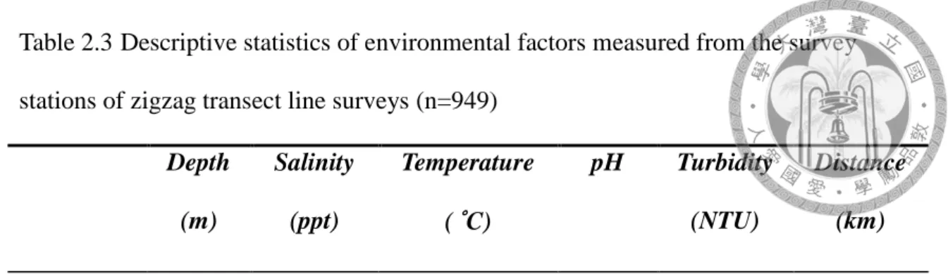
Six environmental factors, e.g. water depth, salinity, temperature, pH value, turbidity, and distance to shore were measured both from the regular survey stations (n=949) as well as from the dolphin contact points (n=23). The average, SE, and 95%
CI range of 6 variables were shown in Table 2.3 and Table 2.4 respectively. The difference between survey stations and dolphins’ contact points environmental characteristics were significant in water depth and distance to shore (Wilcoxon rank sum test, p<0.05), with average of water depth at 7.9 m (95%CI range=6.0-9.7 m) and distance to shore at 2.4 km (95%CI range= 1.3-3.5 km). The frequency distributions of these six factors were compared between datasets of survey stations and contact points of dolphins (Fig. 2.6).
For salinity, both datasets peaked at 31-35 parts per thousand (ppt), but the presence data also showed three minor peaks around 25-30 ppt, indicating an estuarine environment. The temperature distribution exhibited two peaks, indicating the summer and winter seasons of the survey, with a smaller curve for contact points in summer. No major peaks were found in the water depth records, indicating that the sampling stations had an even topology as expected by survey design, but the contact points data was significantly different (Wilcoxon rank sum test, p<0.05) from the survey stations’ data with peaks below 10 meter in depth. Both pH value datasets showed similar patterns with pH around 8 as alkaline, but the contact points curve was a little higher in overall
distance to shore of survey stations distributed from 0 to 15 km, and mostly focused below 6 km. And the distance of contact points were significantly different from survey stations (Wilcoxon rank sum test, p=0.03), and were densely distributed at inshore areas, but there were two points with distance at 7 km and 10 km, which were at Chuoshui River (濁水溪) and most eastern Chiayi water, respectively (Fig. 2.4).
2.3.4 Density and Abundance Estimates from Inshore Parallel Transect Lines
In total 17,257 kilometers of on-effort distance were covered over 394 inshore parallel transect line surveys from 2008 to 2012. The efforts and study area varied from year to year because of the different research projects (Table 2.5). The efforts were abundant between 2008 and 2009, and 2009 in particular held the highest record with the largest surveyed area. From 2010 to 2012, the effort amount and study area remained relatively similar as opposed to the much more intensive surveys of 2008-2009 described above.
To estimate population density, sightings with a perpendicular distance greater than 400m were truncated because the CV was the least among other truncation options.
Among the 9 models, the least AICc model was Hazard-rate without adjustment (Fig.
2.9), which estimated the effective strip width to be 113.63m, density to be 0.31, and the abundance to be 68 (95%CI: 54-85). The coefficient of variance of density and abundance was 11.5% (see Table 2.6 for detail).
Aside from the pooled data, specific estimations of each year were also applied for temporal variation. The truncation principle was the same as above, set at distance
>400m with the least CV. After properly selecting the best-fit models, some key