應用數位相機量測開裂處之應力集中係數

應用數位相機量測開裂處之應力集中係數

計畫類別： 個別型計畫

計畫編號： NSC92-2211-E-006-066-

執行期間： 92 年 08 月 01 日至 93 年 07 月 31 日 執行單位： 國立成功大學土木工程學系（所）

計畫主持人： 朱聖浩

計畫參與人員： 劉淑秀

報告類型： 精簡報告

處理方式： 本計畫可公開查詢

中 華 民 國 93 年 11 月 1 日

應用數位相機量測開裂處之應力集中係數

Measuring stress intensity factors by digital camera

計畫編號：92-2211-E-006-066- 執行期間：2003.08.01 至 2004.07.31

計畫主持人：朱聖浩 國立成功大學土木工程學系教授

關鍵字

數位影像，裂縫，開裂處變位，數位相機，試驗，有限元素法，最小二乘法，應力集中係數。

中文摘要

本論文使用數位相機配合實體顯微鏡來量測試體變位，並用最小二乘法求解開裂處之應力集中係數，

量測試體可為均向性及異向性材料。一般而言，量測的方法很多，但須複雜的步驟或昂貴的儀器，由於 近年來數位相機發展一日千里及物美價廉，其解析度配合實體顯微鏡已可用來量測變位。首先在試體上 貼上基準點，然後使用數位相機配合實體顯微鏡，將變位前後之影像紀錄，由變位前後之影像比對，得 到各點之變位，配合類似有限元素法由變位求應力之步驟，求的開裂處之應力集中係數。本研究之優點 為(1)試驗方法及試體之準備均不複雜，(2)不須使用防振設施，例如防振台等。有限元素法及數位相機 試驗均證明本法正確且精確度不差。

Keywords

Computer image, Crack, Crack opening displacement, Digital camera, Experiment, Finite element method, Least-squares method, Stress intensity factors.

Abstract

This project developed a least-squares method to evaluate the mixed-mode stress intensity factors (SIFs) of a cracked material using the computer images from the digital-camera experiment. This experiment measures the crack opening displacement (COD) and then evaluates SIFs by using the least-squares method. The attractions of this method include: (1) specimen preparation and experiment procedures are not complicated and (2) the isolation of the micro-vibration is not necessary in the experiment. Both finite element simulations and laboratory experiments were applied to validate the current least-squares method with acceptable accuracy, if the even terms of the Irwin’s equation are removed.

1. Introduction

The main purpose of this project is to evaluate in-plane stress intensity factors (SIFs), KI

and K_II, for a centrally-cracked steel plate using the computer images from digital-camera experiments. In the past several years, digital-camera or charge-coupled device (CCD) experiments have been used to fracture mechanics. McNeill et al. (1987) used the computer image correlation of deformed white light speckle patterns in the crack tip to find the SIF.

Experimental data for mode-I cracked body problems were presented and compared their study with acceptable analytical results. Nahm et al. (1996) applied the remote measurement system and image processing technique to study the growth behavior of small surface fatigue cracks in 1Cr -1Mo-0.25V steel. The measurement error of the system appeared to be 0.8%

and the system could measure down to 30 mu m of surface fatigue crack length. Chao et al.

(1998) applied the digital image processing to obtain the deformation fields around a propagating crack tip from photographic films recorded by a high-speed Cranz-Schardin camera. The in-plane displacements and strains determined from the process were then used to computer the dynamic SIF. Semenski and Jecic (1999) used the reflection method of caustics for application to cracks in mechanically anisotropic materials. To find the exact position of caustics, the experimental images were analyzed by the simple boundary value method and a more sophisticated differential method, which is accomplished by shifting the real image onto the gradient image. Takahashi et al. (2000) presented experimental results

which demonstrate restraint of fatigue crack growth in an Al-Mg alloy by wedge effects of fine particles. In their paper, in situ observations of fatigue cracks were performed for the two cases using a CCD microscope, with a magnification of x1000. The crack length and the crack opening displacement (COD) at the notch root were measured. Machida (2000) measured the point-by-point measurement of in-plane displacement using the pointwise filtering approach of speckle photography. Young's fringes patterns were taken by a CCD and analyzed by the image-processing system. Then, stress-intensity factors were evaluated using the displacement data obtained using speckle photography by applying the least-squares method. Lin (2002) used the digital image and multimedia technology projected in a modified laser shadow spot set-up to engage in a model of the crack growth. With a video CCD camera and frame grabber analyzing, a series of images of laser shadow spot during crack growth was used to evaluate the SIF. Oda et al. (2004) analyzed full field infrared radiometry based on thermoelastic and thermoplastic theory for the non-contact evaluation of stress and deformation distributions in mechanically dissimilar material systems. A CCD camera was employed to investigate the crack tip opening displacement (CTOD) for steel plates loaded in uniaxial tension perpendicular to the weld line.

In the literature, determining mixed-mode SIFs using computer images is limited. This study investigates the accuracy of the least-squares method incorporating the image processing technique to solve mixed-mode fracture problems, and micro-vibration isolation is not necessary during the current experiment.

2. Calculating SIFs using least-squares method

The least-squares method has been applied to the thermoelastic experiments and the finite element method for isotropic and composite materials (Ju, 1996; Ju et al., 1997; Ju, 1998; Ju and Rowlands, 2003). In this study, the similar least-squares method incorporating the displacement filed of the isotropic material from the finite element analysis and the digital camera was employed.

2.1 Least-squares method using finite element results

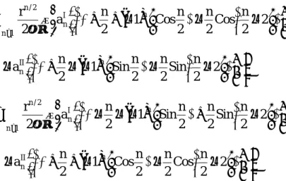
Figure 1 shows an isotropic Infinite plate containing a sharp crack, where x and y are the coordinates of an arbitrary point while the original point of interest is located at the crack tip and the crack surface is in the negative x direction; u and v are the displacement in x and y directions, respectively; r and θare the polar coordinates. The in-plane displacements, u and v, of a cracked isotropic and linear-elastic plate are (Irwin, 1957)

∑

^∞

( )

= 



 

θ



 





−

−



θ



 





κ + + − µ ×

=

1 n

I n n 2 / n

2 2 Cos n 2 n 2 Cosn 2 1

a n 2 u r

( )



 

 

 

θ



 





−

−



θ



 





κ + − −

−

2

2 Sin n 2 n 2 Sinn 2 1

a^II_n n ⁿ (1)

∑

^∞

( )

= 



 

θ



 





− +



θ



 





κ − − − µ ×

=

1 n

I n n 2 / n

2 2 Sin n 2 n 2 Sinn 2 1

a n 2 v r

( )





 

θ



 





−

−



θ



 





κ + + −

−

2

2 Cos n 2 n 2 Cosn 2 1

a^II_n n ⁿ (2)

where

_µ

is shear modulus,

_{κ =} 3 ₋ 4 _ν for plane stress and κ = ( 3 − ν ) /( 1 + ν ) for plane strain, ν is Poisson’s ratio and a and

^I_n

a are parameters to be determined. Particularly, the first

^II_n

terms of parameters are the function of SIFs as follows:

= π 2

a

₁^I

K

^I

and

= π 2

a

₁^II

K

^II

(3)

When the first N terms are selected, the matrix forms of equation (1) and (2) are

[ ^A

¹

^A

²

^{... A}

^N

^B

¹

^B

²

^{... B}

^N

] [ ^a

^1I

^a

^I2

^{... a}

^IN

^a

^1II

^a

^II2

^{... a}

^IIN

]

^T

u =

or u=[A]{a} (4)

[ ^C

¹

^C

²

^{... C}

^N

^D

¹

^D

²

^{... D}

^N

] [ ^a

^1I

^a

^2I

^{... a}

^IN

^a

^1II

^a

^II2

^{... a}

^IIN

]

^T

v =

or v=[C]{a} (5)

where ( ) ^{2 ,}

2 Cos n 2 n 2 Cos n 2 1

n 2

A r

ⁿ

2 / n

n 



_θ



 





₋

−



θ



 





_{κ + + −}

= µ (6)

( ) ^{2 ,}

2 Sin n 2 n 2 Sin n 2 1

n 2

B r

ⁿ

2 / n

n 



_θ



 





₋

−



θ



 





_{κ + − −} µ

= −

( ) ^{2 and}

2 Sin n 2 n 2 Sin n 2 1

n 2

C r

ⁿ

2 / n

n 



_θ



 





₋ +



θ



 





_{κ − − −}

= µ

( ) ^{2 .}

2 Cos n 2 n 2 Cos n 2 1

n 2

D r

ⁿ

2 / n

n 



_θ



 





₋

−



θ



 





_{κ + + −} µ

= −

The error for m nodes with u and v displacements from numerical simulations or experimental measurement is

( ) (

i i

)

²

m 2

1 i

i

i

[ a ] u [ C ] [ a ] v ]

A

[ − + −

= π ∑

=

(7) where u

_i

, v

_i

, [A]

_i

and [C]

_i

are the u, v, [A] and [B] of equations (4) and (5) at node i obtained

from finite element analyses or the experiments.

To minimize the error by using ∂π / ∂ { a } , one obtains

[K]{a

}

={F} (8)

where

_i

m

1 i

T i i T

i

[ A ] [ C ] [ C ] ]

A [ ] K

[ ∑

=

+

= is a symmetric matrix, and {F}=

_i^T

m

1 i

i T i

i

[ A ] v [ C ]

∑ u

=

+ .

In this least-squares method, the parameters N, R

_max

and R

_min

can be adjusted; N is the number of terms in equations (4) and (5), R

_max

and R

min

are the maximum and minimum radius, respectively, of the area from which data will be included. This study uses N=1 to 8, R

max

=the crack length and R

min

=0.01 mm.

2.2 Least-squares method using crack opening displacements from experiments

In the digital-camera experiment of this study, a number of small square symbols on the

project are attached on the specimen with the y-distance,

Δ

y, from the crack surface as

shown in Fig.1. Then, the crack opening displacements (COD) at the symbols in x and y

direction are measured. From equations (4) and (5), the COD between symbols in x and y directions, u ∆ and v ∆ , can be arranged as follows:

[ ^U

¹

^U

²

^{... U}

^N

] [ ^a

^1II

^a

^II2

^{... a}

^IIN

]

^T

u =

∆ or ∆ u = [ U ]{ a

^II

} (9)

[ ^V

¹

^V

²

^{... V}

^N

] [ ^a

^1I

^a

^I2

^{... a}

^IN

]

^T

v =

∆ or ∆ v = [ V ]{ a

^I

} (10)

where ( ) ^{2 ,}

2 Sin n 2 n 2 Sin n 2 1

n

U r

ⁿ

2 / n

n 



_θ



 





₋

−



θ



 





_{κ + − −} µ

= − (11)

( )

_^



_θ



 





₋ +



θ



 





_{κ − − −}

= µ 2

2 Sin n 2 n 2 Sin n 2 1

n

V r

ⁿ

2 / n

n

and

r and θ are located on the non-negative-y-coordinate region.

In the experiment,

Δ

y of Fig.1 is considerably small. If it is zero, θ in equation (11) equals π , which causes zero of U

_n

and V

_n

for even terms. This condition produces large error of the least-squares method. Alternative is to neglect the even terms of equation (9) and (10) as follows:

[ ^U

¹

^U

³

^U

⁵

^U

⁷

^{... U}

^N

] [ ^a

^1II

^a

^II3

^a

^II5

^a

^II7

^{... a}

^IIN

]

^T

u =

∆ or ∆ u = [ U ]{ a

^II

} (12)

[ ^V

¹

^V

³

^V

⁵

^V

⁷

^{... V}

^N

] [ ^a

^1I

^a

^I3

^a

^I5

^a

^7I

^{... a}

^IN

]

^T

v =

∆ or ∆ v = [ V ]{ a

^I

} (13)

where N is odd.

Using the same least-squares method for m pairs of displacement symbols, one obtains

[K

_U

]{a

^II

}={F

_U

} and [K

_V

]{a

^I

}={F

_V

} (14)

where ∑ ∑ ∑ ∑

=

=

=

=

=

=

=

=

^m

1 i

T i i V

m

1 i

T i i U

m

1 i

i T i V

m

1 i

i T i

U

] [ U ] [ U ] , [ K ] [ V ] [ V ] , {F } u [ U ] and {F } v [ V ] .

K

[ (15)

3. Illustration of digital camera experiment 3.1 Specimens

Three A36 steel specimens (300 mm long, 45 mm wide and 6 mm thick) were used in the digital-camera experiment. The central crack is inclined at 0

^o

, 30

^o

or 50

^o

with respect to the horizontal. The cracks (total length 2a=30 mm by 0.3 mm wide) were prepared by electrical discharge machining (EDM). Figure 2 shows one of the specimens with the crack angle of 30

^o

. Along the crack line, two papers containing two lines of square black symbols were attached on the specimen with

Δ

y of 0.5 mm (Fig.1). The length between two symbol centers is 25/69 mm, and the square symbol size is about 0.2 mm. The paper with the thickness of 0.109 mm is commonly used for laser printers. Those square black symbols were printed using a laser printer with the resolution of 600 dpi.

3.2 Digital camera, stereo microscope and illuminant

The Fuji S2 Pro Digital Camera connected to a stereo microscope was used in the experiment as shown in Fig.3. This camera with 4,256x2,848-pixel maximum resolution is controlled by a camera shooting software in a personal computer using a direct IEEE1394 cable connection. The shutter speed of 1/125 second and ISO-800 were set in the experiment.

The image is saved in the uncompressed TIFF file. The magnification of the stereo

microscope is from 7 to 45 times. In the experiment, the working distance between the

specimen surface and the microscope edge is about 100 mm with the magnification of 40 times, which can cover the image area of 3 mm by 2 mm for the whole resolution of 4,256x2,848-pixel. The digital camera and stereo microscope are supported on a tripod and allow the adjustment on both horizontal and the vertical directions. The illuminant is two optical-fiber lights transferred from a 20V-150-W halogens lamp.

3.3 Experimental procedures

The experiment was performed using the Inston-8800 servohydraulic testing machine with a load cell of 100-KN capacity under load control without vibration isolation schemes. The procedures for the experiment are listed below:

(1) Mount the specimen (see Fig.2) and adjust the microscope-digital-camera system to obtain an image with the area of 3 mm by 2 mm approximately (8 square symbols in the x direction (Fig.4)). At the first time, the image is located near the crack tip.

(2) Set to zero load, and take a picture from the digital camera using the camera shooting software in a personal computer. Then increase load to 10, 15 and 20 kN (stress of 37.04, 55.56 and 74.07 N/mm

²

) to take pictures, respectively. All the pictures are stored with the TIFF format.

(3) Adjust the tripod, so the microscope-digital-camera system is allowed to move to the next section for observation (gradually move to the crack center), and then repeat procedure (2) . After the image near the crack center is taken, stop the test.

3.4 Evaluation of displacements from computer images

After the experiment, a Fortran program CCD3 (http//myweb.ncku.edu.tw/~juju/index.htm) can be used to calculate the x and y centers of the square symbols of each picture. The displacements at the centers of those square symbols are obtained from their coordinate difference between the W-load and zero-load pictures, where W is the load of 10, 15 or 20 kN used in this project. Thus, CODs in x and y directions are calculated from the displacement difference between upper and bottom square symbols. The procedures of the program CCD3 are illustrated as follows:

(1) Read the TIFF file and obtain the red, green and blue (RGB) values at each pixel (totally, 4,256x2,848 pixels). Subroutine RIMAGE (about 120 statements) in CCD3 program performs this procedure.

(2) This step finds the region of each square symbol. Since the RGB values of the pixels in a square symbol are much different from those of other place. The CCD3 program finds the regions that have the similar RGB value of the square block. The programming algorithm is similar to the polygon filling of the computer graphics. Subroutine GP (about 100 statements) in CCD3 program performs this procedure. Since the symbol area and size are known, too large or too small regions that are noises or wrong regions will be skipped.

(3) Calculate the x and y centers of each region of the square symbol for this current picture.

We must note that the size of the square symbol is too small (about 0.2 mm), so it is often not a good square shape. This situation will not cause trouble, since the CCD3 program can find the region that has the certain RGB values, and the square shape is not necessary.

(4) Go to step 1 for the next picture. Until finishing the last picture, stop the program.

Figure 4a and 4b shows the images (TIFF files) taken from the digital camera for the

specimen with the crack angle of 30

^o

under the loads of 0 and 20 kN. Figure 4c shows the

positions of square symbols under 0 and 20 kN using the CCD3 program. The displacement

of each symbol can be clearly seen in Fig.4c.

4 Numerical validation

Numerical experiments were conducted initially using the finite element analysis.

These finite element predictions provide the input for equation (8) as well as the simulated experimental input COD values for equation (14). Eight-node quadrilateral isoparametric elements were utilized in the finite element meshes; furthermore, quarter-point singular isoparametric elements (Henshell and Shaw, 1975) were employed around the crack tip. All numerical experiments assume linear-elastic, plane-stress conditions. The applied stress, S, in each case is unity and the material is steel (Young’s modulus E=204 Gpa and Poisson’s ratio v=0.29).

The problem is a center slant cracked rectangular plate subjected to uniform unixial tensile stress as shown in Fig.5a. The SIFs of this problem were solved by Kitagawa and Yuuki (1977) using the modified mapping collocation method. The crack angle ( α ) is set to 15

^o

, 30

^o

or 60

^o

, and the crack length over the specimen width (a/W) is set to 0.4, 0.6 or 0.7.

The finite element mesh near the crack of α ⁼³⁰

^o

and a/W=0.7 is shown in Figs.5b. The error of the least-squares method and the equivalent SIFs are defined as follows:

f Re

LS f Re

K K

Error K −

= (16)

) a S /(

K

F_I

=

_I^LS

π ^and

F_II

=

K_II^LS/(S

π

a)

⁽¹⁷⁾ where

K^Ref

is the stress intensity factor K

I

or K

II

obtained from the reference (Kitagawa and Yuuki, 1977),

K^LS

is that calculated from the least-squares method, S is the applied stress at far field and a is the crack length.

4.1 Accuracy of the least-squares method using finite element results

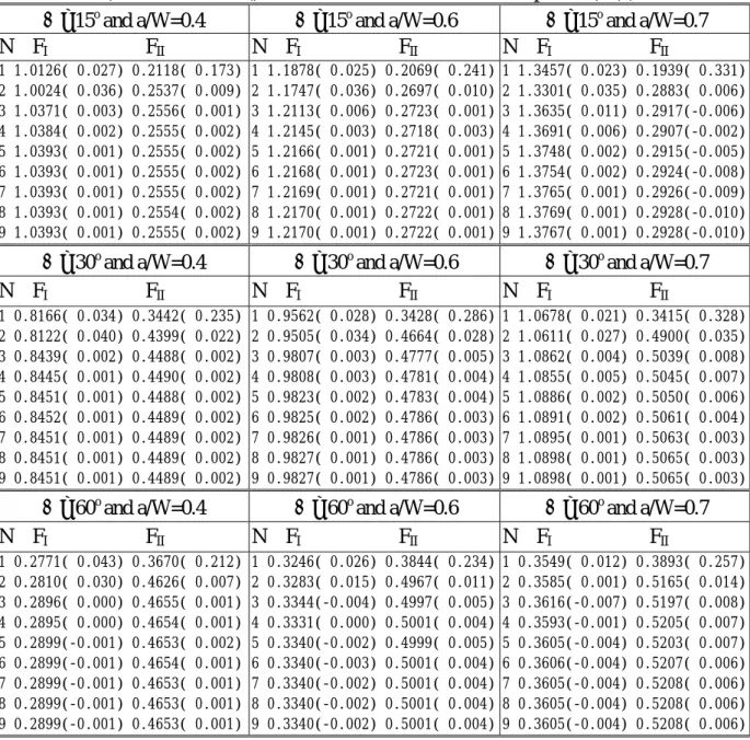
The variations of SIFs affected by N (from 1 to 9) were investigated as shown in Table 1 using equation (8), where the SIFs of Table 1 are averaged under R

_max

=2mm, 5 mm and 10 mm and R

_min

=0.01 mm. Table 1 indicates that the least-squares results agree well with the referenced SIFs except N

≦

2. This means that the least-square method incorporating the finite element result can evaluate the SIFs accurately for N

≧

3. Moreover, the accuracy is also independent of R

max

. For practice, R

max

should be smaller than the crack length to avoid including other singular data and R

_min

can equal a very small value to only exclude the singularity at the crack tip.

4.2 Accuracy of the least-squares method using simulated COD values

The least-squares method of equations in section 2.2 is used with the simulated COD from finite element results. Since experimental input values usually contain some scatter error, those simulated COD data from finite element analyses were subsequently modified according to the following equation.

S=S

_original

(1+RAN*P

_factor

) (18)

where values of S computed by equation (18) now become the input for the least-squares method, such that S

_original

is the ‘perfect’ x- or y-COD obtained from the finite element analysis; RAN is a random value between –1 and 1, and P

_factor

is a user-selected factor. In this study P

_factor

is set to 0, 0.1 and 0.4, in which 0.4 means that the maximum error over S

original

can extend to 40%.

The variations of SIFs affected by P

_factor

(0, 0.1 and 0.4), N (from 1 to 9) and

Δ

y (0, 0.25

and 0.5 mm; Fig.1) were investigated under the combinations of three crack angles of 15

^o

, 30

^o

or 60

^o

and three a/W of 0.4, 0.6 or 0.7, so there are total 9 cases for a certain P

factor

, N and

Δ

y.

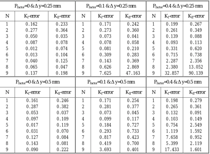
First, equations (9), (10) and (14) are used, which means that the even terms are not removed.

At this condition, equation (14) is singular for

Δ

y=0 and no solution can be obtained. For

Δ

y=0.25 and 0.5 mm, Table 2 shows the averaged errors of least-squares results, where the averaged error is the mean error value (equation (16)) of the 9 cases (the combinations of three crack angles and three a/W). Table 2 shows the following features:

(1) For P

factor

=0 and N=1 or 2, the errors are large and generally the calculated SIFs cannot be used. For N>2, the errors are still much larger than those of Table 1, which means that the least-squares results are not stable when equations (9) and (10) are applied.

(2) When a small scatter error is given (P

factor

=0.1), the errors of least-squares results increasing proportional to N are considerably large except for N=3. For a larger scatter error (P

_factor

=0.4), the condition is even worse.

(3) Generally, the errors are larger for smaller

Δ

y. The reason is because a smaller

Δ

y produces more singular result of equation (14).

Table 1. Least-squares results and errors of numerical experiments (The value inside () means the error calculated from equation (16).) 15

o

=

α and a/W=0.4 α = 15

^o

and a/W=0.6 α = 15

^o

and a/W=0.7 N F

I

F

II

N F

I

F

II

N F

I

F

II 1 1.0126( 0.027) 0.2118( 0.173)

2 1.0024( 0.036) 0.2537( 0.009) 3 1.0371( 0.003) 0.2556( 0.001) 4 1.0384( 0.002) 0.2555( 0.002) 5 1.0393( 0.001) 0.2555( 0.002) 6 1.0393( 0.001) 0.2555( 0.002) 7 1.0393( 0.001) 0.2555( 0.002) 8 1.0393( 0.001) 0.2554( 0.002) 9 1.0393( 0.001) 0.2555( 0.002)

1 1.1878( 0.025) 0.2069( 0.241) 2 1.1747( 0.036) 0.2697( 0.010) 3 1.2113( 0.006) 0.2723( 0.001) 4 1.2145( 0.003) 0.2718( 0.003) 5 1.2166( 0.001) 0.2721( 0.001) 6 1.2168( 0.001) 0.2723( 0.001) 7 1.2169( 0.001) 0.2721( 0.001) 8 1.2170( 0.001) 0.2722( 0.001) 9 1.2170( 0.001) 0.2722( 0.001)

1 1.3457( 0.023) 0.1939( 0.331) 2 1.3301( 0.035) 0.2883( 0.006) 3 1.3635( 0.011) 0.2917(-0.006) 4 1.3691( 0.006) 0.2907(-0.002) 5 1.3748( 0.002) 0.2915(-0.005) 6 1.3754( 0.002) 0.2924(-0.008) 7 1.3765( 0.001) 0.2926(-0.009) 8 1.3769( 0.001) 0.2928(-0.010) 9 1.3767( 0.001) 0.2928(-0.010)

30

o

=

α and a/W=0.4 α = 30

^o

and a/W=0.6 α = 30

^o

and a/W=0.7 N F

_I

F

_II

N F

_I

F

_II

N F

_I

F

_II

1 0.8166( 0.034) 0.3442( 0.235) 2 0.8122( 0.040) 0.4399( 0.022) 3 0.8439( 0.002) 0.4488( 0.002) 4 0.8445( 0.001) 0.4490( 0.002) 5 0.8451( 0.001) 0.4488( 0.002) 6 0.8452( 0.001) 0.4489( 0.002) 7 0.8451( 0.001) 0.4489( 0.002) 8 0.8451( 0.001) 0.4489( 0.002) 9 0.8451( 0.001) 0.4489( 0.002)

1 0.9562( 0.028) 0.3428( 0.286) 2 0.9505( 0.034) 0.4664( 0.028) 3 0.9807( 0.003) 0.4777( 0.005) 4 0.9808( 0.003) 0.4781( 0.004) 5 0.9823( 0.002) 0.4783( 0.004) 6 0.9825( 0.002) 0.4786( 0.003) 7 0.9826( 0.001) 0.4786( 0.003) 8 0.9827( 0.001) 0.4786( 0.003) 9 0.9827( 0.001) 0.4786( 0.003)

1 1.0678( 0.021) 0.3415( 0.328) 2 1.0611( 0.027) 0.4900( 0.035) 3 1.0862( 0.004) 0.5039( 0.008) 4 1.0855( 0.005) 0.5045( 0.007) 5 1.0886( 0.002) 0.5050( 0.006) 6 1.0891( 0.002) 0.5061( 0.004) 7 1.0895( 0.001) 0.5063( 0.003) 8 1.0898( 0.001) 0.5065( 0.003) 9 1.0898( 0.001) 0.5065( 0.003)

60

o

=

α and a/W=0.4 α = 60

^o

and a/W=0.6 α = 60

^o

and a/W=0.7 N F

I

F

II

N F

I

F

II

N F

I

F

II 1 0.2771( 0.043) 0.3670( 0.212)

2 0.2810( 0.030) 0.4626( 0.007) 3 0.2896( 0.000) 0.4655( 0.001) 4 0.2895( 0.000) 0.4654( 0.001) 5 0.2899(-0.001) 0.4653( 0.002) 6 0.2899(-0.001) 0.4654( 0.001) 7 0.2899(-0.001) 0.4653( 0.001) 8 0.2899(-0.001) 0.4653( 0.001) 9 0.2899(-0.001) 0.4653( 0.001)

1 0.3246( 0.026) 0.3844( 0.234) 2 0.3283( 0.015) 0.4967( 0.011) 3 0.3344(-0.004) 0.4997( 0.005) 4 0.3331( 0.000) 0.5001( 0.004) 5 0.3340(-0.002) 0.4999( 0.005) 6 0.3340(-0.003) 0.5001( 0.004) 7 0.3340(-0.002) 0.5001( 0.004) 8 0.3340(-0.002) 0.5001( 0.004) 9 0.3340(-0.002) 0.5001( 0.004)

1 0.3549( 0.012) 0.3893( 0.257) 2 0.3585( 0.001) 0.5165( 0.014) 3 0.3616(-0.007) 0.5197( 0.008) 4 0.3593(-0.001) 0.5205( 0.007) 5 0.3605(-0.004) 0.5203( 0.007) 6 0.3606(-0.004) 0.5207( 0.006) 7 0.3605(-0.004) 0.5208( 0.006) 8 0.3605(-0.004) 0.5208( 0.006) 9 0.3605(-0.004) 0.5208( 0.006)

Table 2. Averaged errors of least-squares results using equations (9), (10) and (14) (averaged error is the mean value of equation (16) for the 9 cases from the combinations of

three crack angles and three a/W.)

P_factor=0 &Δy=0.25 mm P_factor=0.1 &Δy=0.25 mm P_factor=0.4 &Δy=0.25 mm

N K_I-error K_II-error N K_I-error K_II-error N K_I-error K_II-error 1

2 3 4 5 6 7 8 9

0.162 0.277 0.050 0.087 0.012 0.013 0.040 0.065 0.137

0.233 0.364 0.035 0.078 0.074 0.104 0.125 0.047 0.198

1 2 3 4 5 6 7 8 9

0.171 0.273 0.073 0.078 0.081 0.309 0.143 0.626 7.625

0.242 0.360 0.041 0.058 0.210 0.283 0.369 2.869 47.163

1 2 3 4 5 6 7 8 9

0.199 0.261 0.139 0.093 0.331 0.715 2.287 2.380 32.857

0.267 0.349 0.088 0.113 0.620 0.738 2.356 13.052 90.139

P_factor=0 &Δy=0.5 mm P_factor=0.1 &Δy=0.5 mm P_factor=0.4 &Δy=0.5 mm

N K_I-error K_II-error N K_I-error K_II-error N K_I-error K_II-error 1

2 3 4 5 6 7 8 9

0.161 0.287 0.053 0.097 0.017 0.031 0.127 0.143 0.090

0.246 0.382 0.037 0.109 0.119 0.070 0.084 0.081 0.222

1 2 3 4 5 6 7 8 9

0.171 0.281 0.073 0.099 0.184 0.293 0.817 0.419 3.693

0.254 0.377 0.045 0.117 0.727 0.733 0.423 0.700 0.401

1 2 3 4 5 6 7 8 9

0.198 0.265 0.132 0.103 0.754 1.119 7.658 5.399 17.433

0.279 0.361 0.091 0.149 2.549 1.592 0.952 2.119 1.601

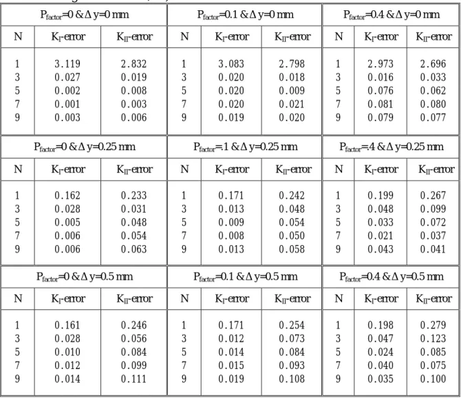
Then, equations (12), (13) and (14) are used, which means that the even terms are removed. At this condition, equation (14) will not be singular for

Δ

y=0. Table 3 shows the averaged errors of least-squares results, which indicate the following features:

(1) For P

factor

=0 and N=1, the error is large and generally the calculated SIFs cannot be used.

For N

≧

3, the errors are small and similar to those of Table 1, which means that the least-squares results are stable when even terms are removed.

(2) Although the least-squares errors increase slowly proportional to P

factor

, they are not sensitive to the scatter errors. This means that the least-squares method using equations (12) and (13) can average the scatter errors of the input data. When scatter errors are large but averaged values of them are small, which means that the measured data are located positively and negatively along the correct data, the errors of this least-squares method can be small too.

(3) Generally, the error is larger for a larger

Δ

y. The reason is because the least-squares method using equations (12) and (13) that remove the zero terms is only correct for

Δ

y=0.

When

Δ

y increases, the approximation intensity of the least-squares method using

equations (12) and (13) will also increase. Thus, when

Δ

y is not large, the accuracy of

this least-squares method can be acceptable.

Table 3. Averaged errors of least-squares results using equations (12), (13) and (14) (averaged error is the mean value of equation (16) for the 9 cases from the combinations of three crack angles and three a/W.)

P_factor=0 &Δy=0 mm P_factor=0.1 &Δy=0 mm P_factor=0.4 &Δy=0 mm

N K_I-error K_II-error N K_I-error K_II-error N K_I-error K_II-error 1

3 5 7 9

3.119 0.027 0.002 0.001 0.003

2.832 0.019 0.008 0.003 0.006

1 3 5 7 9

3.083 0.020 0.020 0.020 0.019

2.798 0.018 0.009 0.021 0.020

1 3 5 7 9

2.973 0.016 0.076 0.081 0.079

2.696 0.033 0.062 0.080 0.077

P_factor=0 &Δy=0.25 mm P_factor=.1 &Δy=0.25 mm P_factor=.4 &Δy=0.25 mm

N KI-error KII-error N KI-error KII-error N KI-error KII-error 1

3 5 7 9

0.162 0.028 0.005 0.006 0.006

0.233 0.031 0.048 0.054 0.063

1 3 5 7 9

0.171 0.013 0.009 0.008 0.013

0.242 0.048 0.054 0.050 0.058

1 3 5 7 9

0.199 0.048 0.033 0.021 0.043

0.267 0.099 0.072 0.037 0.041

P_factor=0 &Δy=0.5 mm P_factor=0.1 &Δy=0.5 mm P_factor=0.4 &Δy=0.5 mm

N K_I-error K_II-error N K_I-error K_II-error N K_I-error K_II-error 1

3 5 7 9

0.161 0.028 0.010 0.012 0.014

0.246 0.056 0.084 0.099 0.111

1 3 5 7 9

0.171 0.012 0.014 0.015 0.019

0.254 0.073 0.084 0.093 0.108

1 3 5 7 9

0.198 0.047 0.024 0.040 0.035

0.279 0.123 0.085 0.075 0.100

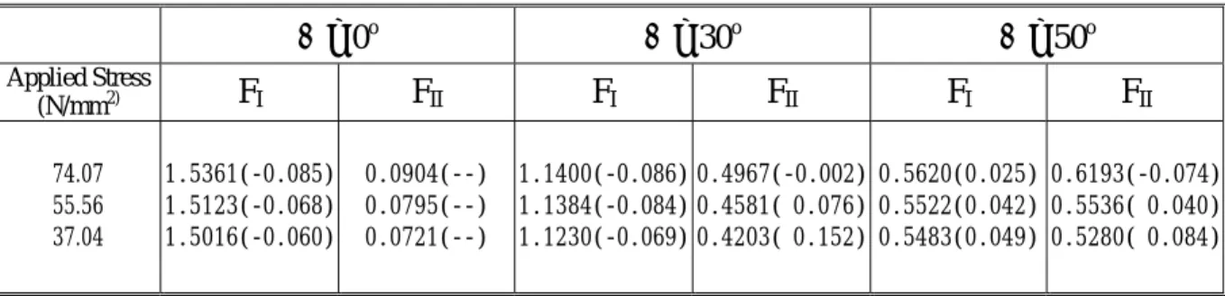
5. Experimental results

In this section, the least-squares method is applied to evaluate the SIFs of the

experiments illustrated in section 3. Figure 6 shows parts of the CODs measured by the digital

camera and calculated by the finite element method. This figure indicates that the two results

are in good agreement. For the digital-camera experiment, the least-squares results are the

averaged values under N=3, 5 and 7 using equations (12), (13) and (14) (even terms are

removed). The referenced SIFs for comparison as shown in Table 4 are calculated using the

least-squares method of equation (8) with the condition of R

_max

=5 mm, R

_min

=0.01 mm and

N=8. Table 5 shows the experimental results evaluated by the least-squares method. This table

indicates that the SIF error of the digital-camera experiment is about 8%, which should be

acceptable for the mixed-mode fracture problem. From out further investigation, most of the

errors or scatters of experiment results are due to the distortion of the microscope. This

condition can sometimes produce about 2-pixel difference between a certain location. The

micro-vibration and illumination of the experimental system are not dominated. Thus, to

improve the experimental accuracy, it is suggested that a precise micro-scope or a distortion

calibration procedure be used.

Table 4. Least-squares SIFs using finite element analyses for specimens in Fig.2 0

o

=

α α = 30

^o

α = 50

^o

F

I

F

II

F

I

F

II

F

I

F

II

1.416 0.000 1.050 0.4958 0.5786 0.5765

Table 5. Least-squares SIFs using experimental results for specimens in Fig.2 (The value inside () means the error calculated from equation (16), where K

^Ref

is obtain from Table 4.)

0

o

=

α α = 30

^o

α = 50

^o

Applied Stress

(N/mm²⁾

F

I

F

II

F

I

F

II

F

I

F

II

74.07 55.56 37.04

1.5361(-0.085) 1.5123(-0.068) 1.5016(-0.060)

0.0904(--) 0.0795(--) 0.0721(--)

1.1400(-0.086) 1.1384(-0.084) 1.1230(-0.069)

0.4967(-0.002) 0.4581( 0.076) 0.4203( 0.152)

0.5620(0.025) 0.5522(0.042) 0.5483(0.049)

0.6193(-0.074) 0.5536( 0.040) 0.5280( 0.084)

6. Conclusion

This project developed a least-squares method to find the mixed-mode SIFs of the isotropic material using the digital-camera experiment, in which two papers containing two lines of square black symbols were attached on the specimen along the crack. Then, a digital camera connected to a stereo microscope was used to measure the displacement of each symbol so that the CODs of the crack can be evaluated. Finally, the least-squares method was applied to calculate SIFs using the measured CODs. Finite element simulations and laboratory experiments were performed to validate that the accuracy of the current least-squares method is acceptable if the even terms of the Irwin’s equation (Irwin, 1957) are removed. The advantages of this method include: (1) specimen preparation and experiment procedures are not complicated and (2) the isolation of the micro-vibration is not necessary, if the shutter speed is appropriately arranged, and normally 1/60 to 1/125 second can be set when a servohydraulic testing machine is used.

References

Chao, Y.J., Luo, P.F. and Kalthoff, J.F., 1998. An experimental study of the deformation fields around a propagating crack tip. Experimental Mechanics 38, 79-85.

Henshell, R.D. and Shaw, K.G., 1975. Crack tip elements are unnecessary. International Journal for Numerical Method in Engineering 9, 495-509.

Irwin, G.R., 1957. Analysis of stresses and strains near the end of a crack traveling a plate Trans. ASME Journal of Applied Mechanics.

Ju, S.H., 1996. Simulating stress intensity factors for anisotropic materials by the least squares method. International Journal of Fracture 81, 283-297.

Ju, S.H., J.R. Lesniak and B.I. Sandor, 1997. Finite element simulation of stress intensity factors via the thermoelastic technique. Experimental Mechanics SEM 37, 278-284.

Ju, S.H., 1998. Simulating three-dimensional stress intensity factors by the least-squares Method. International Journal for Numerical Method in Engineering 43, 1437-1451.

Ju S.H. and Rowlands R.E., 2003. Thermoelastic Determination of K_I and K_II in an

Orthotropic Graphite/Epoxy Composite. Journal of Composite Materials 37,2011-2025 .

Kitagawa, H. and Yuuki, R., 1977. Analysis of Arbitrarily shaped crack in a finite plate using conformal mapping, 1^st report-construction of analysis procedure and its applicability. Trans. Apan Soc. Mech. Engrs 43,

4354-4362.

Lin CS, 2002. Pilot-type scientific experimental device using optical method and computer vision

technology. INDILAN Journal of Pure & Applied Physics 40, 816-827 NOV.

Machida K, 2000. Study of stress-analyzing system by speckle photography. JSME International Journal Series A-Solid Mechanics and Material Engineering 43, 343-350 .

McNeill, S.R., Peters, W.H. and Sutton, M.A., 1987. Estimation of stress intensity factor bu digital image correlation. Engineering Fracture Mechanics 28, 101-112.

Nahm SH, Lee HM, Suh CM, 1996. A study on observation and growth behavior of small surface cracks by remote measurement system. KSME Journal 10, 396-404.

Oda I, Willett A, Yamamoto M, Matsumoto T, Sosogi Y, 2004. Non-contact evaluation of stresses and deformation behaviour in pre-cracked dissimilar welded plates. Engineering Fracture Mechanics 71, 1453-1475.

Semenski D, Jecic S, 1999. Experimental caustics analysis in fracture mechanics of anisotropic materials.

Experimental Mechanics 39,177-183.

Takahashi I, Takahashi C, Kotani N , 2000. Restraint of fatigue crack growth by wedge effects of fine particles.

Fatigue & Fracture of Engineering Materials & Structures 23,867-877.

v u

x y

r θ

∆

y

Cr ack sur fa ce

Cr a ck t ip

Fig.1 Infinite plate containing a sharp crack

Fig.2 Details of the A36 steel specimen with the crack angle of 30

^o

(300 mm long, 45 mm wide, 6 mm thick and crack length a=15 mm)

Stereo microscope

Digital camera

Illumina Inston-8800

specimen

Optical-fiber lights

Fig.3 Details of the experimental system

(a) Image from the digital camera (TIFF file) without load

(b) Image from the digital camera (TIFF file) under the load of 20 kN

(c) Image from the CCD3 program under loads of 0 and 20 kN

Fig.4 Computer images taken from the digital camera and generated from the CCD3 program

for the specimen with the crack angle of 30

^o

under loads of 0 and 20 kN

2a

2W

α 2H S= 1

(a) Model illustration for the problems of numerical validation (H=2W)

(b) Finite element mesh of near the crack of α ⁼³⁰

^o

and a/W=0.7

Fig.5 Model and finite element mesh of a center slant cracked rectangular plate subjected to

uniform unixial tensile stress for numerical validation

(a) y-COD under load of 10, 15 or 20 kN for crack angle of 0

^o

(b) x- and y-COD under load of 20 kN for crack angle of 30

^o

(c) x- and y-COD under load of 10 kN for crack angle of 50

^o

Fig.6 Comparison of CODs between experimental and finite element results