線性轉換模型之統計推論

全文

(1)國立交通大學統計學研究所碩士論文. 線性轉換模型之統計推論 Statistical Inference for Linear Transformation Models. 研究生：林泰佐指導教授：王維菁博士. 中華民國九十七年六月.

(2) 線性轉換模型之統計推論 Statistical Inference for Linear Transformation Models. 研究生：林泰佐. Student：Tai-Tso Lin. 指導教授：王維菁博士. Advisor：Dr. Weijing Wang. 國立交通大學統計學研究所碩士論文. A Thesis Submitted to Institute of Statistics College of Science National Chiao Tung University in partial Fulfillment of the Requirements for the Degree of Master in Statistics June 2008 Hsinchu, Taiwan, Republic of China. 中華民國九十七年六月.

(3) 線性轉換模型之統計推論學生: 林泰佐. 指導教授: 王維菁博士. 國立交通大學統計學研究所. 摘. 要. 線性轉換模型是相當彈性的半母數迴歸模型。倖存分析常見的 Cox 模型與 Odds 模型，皆是線性轉換模型的特例。近年來許多研究針對線性轉換模型提出半母數推論方法，一套分析方法卻有廣泛的應用價值，是其吸引人的地方。我們以古典推論理論的兩個原則(動差法和概式法)為架構，檢視現有文獻的建構方式，希望此統整的角度有助辨識不同方法的特質。此外針對設限資料，我們除了討論現有文獻的做法外，並提出一個新的方法。所有的方法均透過模擬實驗檢驗其表現。. 關鍵詞: Cox PH 模型; Odds 模型; 動差法. i.

(4) Statistical Inference for Linear Transformation Models Student: Tai-Tso Lin Advisor: Dr. Weijing Wang. Institute of Statistics Nation Chiao Tung University Hsinchu, Taiwan. ABSTRACT The linear transformation model, which includes the proportional hazard model and the proportional odds model, has received considerable attentions in recent years due to its flexibility. In the thesis, we consider semi-parametric estimation for the regression parameter. We review existing literature under the framework of classical inference theory. Specifically we will see how these “old” principles, namely method of moment and likelihood estimation, are applied to the modern estimation problem which involves an infinite dimensional nuisance parameter in the model formulation. After examining common techniques of handling censored data, we also propose a new approach. All the methods are evaluated by Monte Carlo simulations.. Key words: Cox proportion hazard model; Proportional odds model; Counting process; Inverse probability weighting; Method of moment; Profile likelihood.. ii.

(5) 誌. 謝. 兩年前，懵懵懂懂的我因為自己對數字的高敏感度以及對機率統計這門科學的熱愛，使我發奮努力成為交大統研所的一員。這兩年寶貴的學習時光中，我時常砥礪自己要好好學習並且自動自發，在教授們辛勤的教導與同學們相互研究討論，以及所上提供良好的學習與研究環境(每週清交合作演講、電腦機房和所圖)，使我吸收到很多寶貴的知識與想法。統計是一門應用相當廣泛的科學，促使我更加努力學習其他方面的知識，自我學習能力是我這兩年最大的收穫。古人云：『學海無涯』，我將會繼續保持一個謙卑學習的態度面對接下來的任何挑戰。這篇論文的完成，我最想要感謝我的指導老師王維菁教授這一年來諄諄教誨。老師十分強調正確的研究態度，任何事情都是從最簡單且最直覺的想法開始，想清楚其中的脈絡與思緒是最重要的。因此，在教授的指導協助下，從一開始概念的釐清、建構研究架構直到論文撰寫完成，在這從無到有的過程中，使我學習到面對問題時該有的正確態度。這兩年研究生活中，還要感謝我的好伙伴文廷，不管在學習、研究或生活上，他時常提供我意見與想法。讓我最欽佩的就是他如拼命三郎的學習態度，無形中也激勵我向上，文廷可以說是我的益友也是良師。此外還要感謝仲竹、翁賢、昱緯、重耕和瑜達，雖然我們研究的領域不同，不過大家一起努力一起學習，交換各種意見與心得，並且閒暇之餘聚在一起閒話家常，使我兩年研究生活增添許多歡樂。另外還有研究室的夥伴們－夙吟、政言、香菱、珮琦、佩芳、鈺婷、彥銘、郃嵐和健鈞，謝謝大家的陪伴，讓我在交大的研究生活更加多采多姿。感謝女友姮君在我遇到困難失落難過的時候陪伴我鼓勵我，讓我更加成長茁壯。最後要感謝我最親愛的家人，一路上栽培我的爸爸和媽嗎，以及陪伴我成長的哥哥和弟弟，你們是我最強而有力的後盾。同時感謝口試委員陳鄰安教授、黃信誠教授和王秀瑛教授提供諸多建議，使得本論文更加完善。最後，謹將此論文獻給敬愛的父母親和王維菁教授，感謝他們的無私奉獻，因為有他們對我的栽培與指導，使我不怕面對未來的艱困與挑戰。希望所有關心我的人，能一同分享此篇論文完成之喜悅與榮耀，謝謝大家。. 林泰佐謹誌于國立交通大學統計研究所中華民國九十七年六月 iii.

(6) Contents 摘要 ............................................................................................................................................... i ABSTRACT................................................................................................................................. ii 誌謝 ............................................................................................................................................. iii List of Tables .............................................................................................................................. vi Introduction........................................................................................................ 1. Chapter 1 1.1. Motivation................................................................................................................ 1. 1.2. Inference Methods .................................................................................................. 2. 1.3. Outline ..................................................................................................................... 3 An Overview of Survival Analysis .................................................................... 4. Chapter 2 2.1. Likelihood Inference............................................................................................... 4. 2.2. Nonparametric Estimation..................................................................................... 4. 2.3. Counting Process..................................................................................................... 6 Regression Analysis without Censoring........................................................... 8. Chapter 3. Moment-based Inference........................................................................................ 8. 3.1. 3.1.A The pairwise order indicator as the chosen response .................................... 9 3.1.B The at-risk process as the chosen response ..................................................... 9 3.1.C The counting process as the chosen response ............................................... 10 Likelihood Inference............................................................................................. 11. 3.2. Regression Analysis with Right Censoring.................................................... 12. Chapter 4 4.1. Moment-based Inference...................................................................................... 12 4.1.A The pairwise order indicator as the chosen response .................................. 13 4.1.B The at-risk process as the chosen response ................................................... 16 4.1.C The counting process as the chosen response ............................................... 17. 4.2. Likelihood Inference............................................................................................. 17 4.2.1. Partial Likelihood – Cox model............................................................... 17 iv.

(7) 4.2.2. Conditional Profile Likelihood ................................................................ 18. Chapter 5. New Proposed Method..................................................................................... 20. Chapter 6. Simulation......................................................................................................... 23. 6.1. Cox proportional hazard model .......................................................................... 23. 6.2. Discussion .............................................................................................................. 23. Chapter 7. Concluding Remarks ....................................................................................... 29. Appendix.................................................................................................................................... 30 References.................................................................................................................................. 35. v.

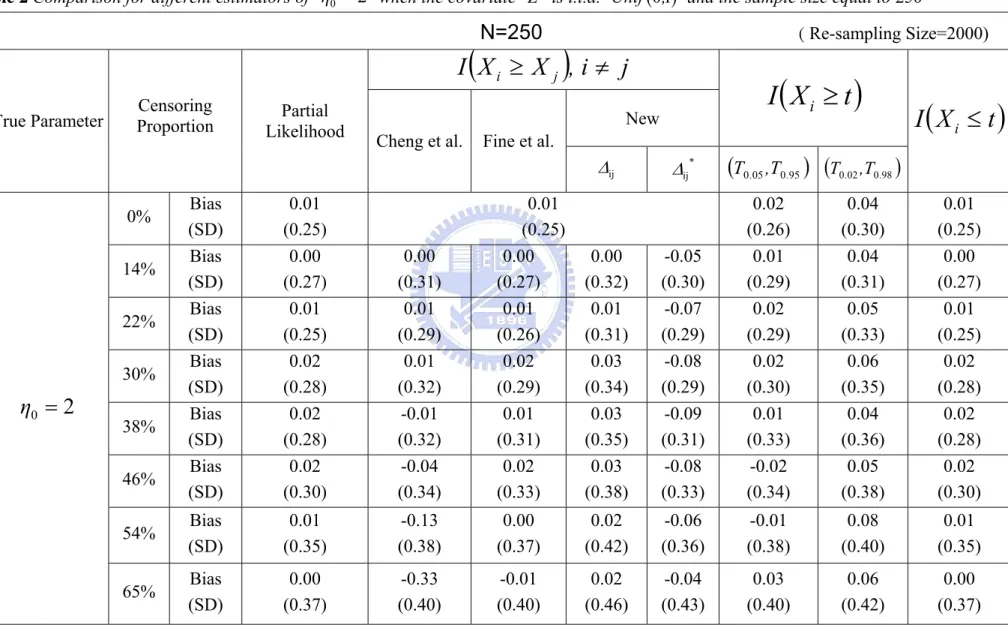
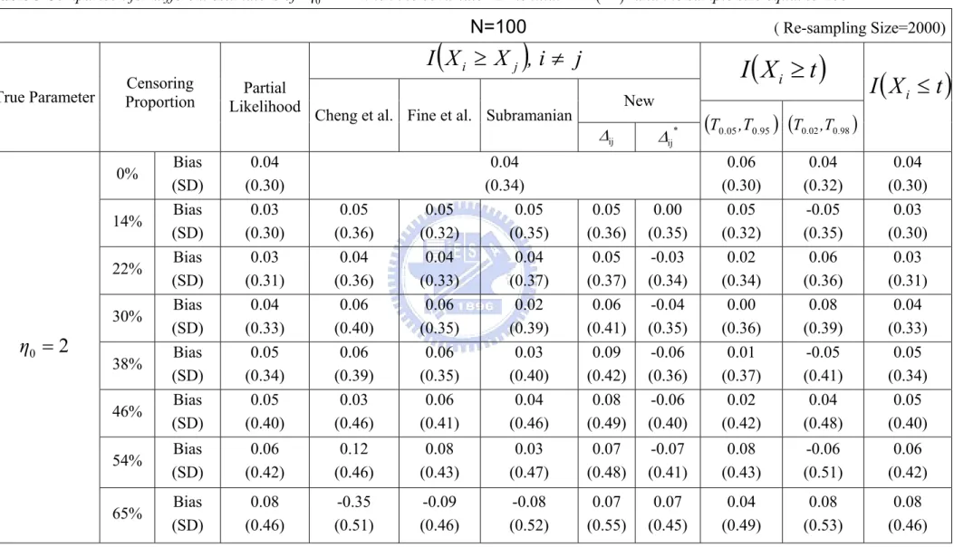
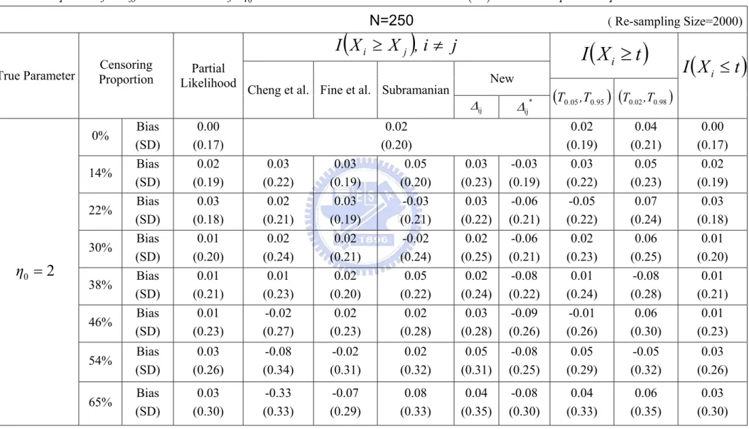
(8) List of Tables TABLE 1 COMPARISON FOR DIFFERENT ESTIMATORS OF η0 = 2. WHEN THE COVARIATE. Z IS I.I.D.. Unif (0,1) AND THE SAMPLE SIZE EQUAL TO 100 ..................................................................... 25 TABLE 2 COMPARISON FOR DIFFERENT ESTIMATORS OF η0 = 2. WHEN THE COVARIATE. Z IS I.I.D.. Unif (0,1) AND THE SAMPLE SIZE EQUAL TO 250 ..................................................................... 26 TABLE 3 COMPARISON FOR DIFFERENT ESTIMATORS OF η0 = 2. WHEN THE COVARIATE. Z IS I.I.D.. Ber(0.5) AND THE SAMPLE SIZE EQUAL TO 100 ...................................................................... 27 TABLE 4 COMPARISON FOR DIFFERENT ESTIMATORS OF η0 = 2. WHEN THE COVARIATE. Z IS I.I.D.. Ber(0.5) AND THE SAMPLE SIZE EQUAL TO 250 ...................................................................... 28. vi.

(9) Chapter 1. Introduction. 1.1 Motivation In many biomedical applications, researchers are interested in studying how covariates affect a patient’s survival time. Let T be the failure time of interest and Z be a p × 1 vector of covariates. The most well-known regression model in survival analysis is perhaps the proportional hazard (PH) model proposed by Cox (1972) which can be written as. λ (t | Z ) = λ0 (t ) × e Z η , T. (1.1). where λ (t | Z) is the hazard function given Z and λ0 (t ) is the hazard for the “baseline” group with Z = (0,0,...,0 ) . The Cox model can also be written as T. log(-log{S (t | Z )}) = log (Λ0 (t )) + Z T η ,. (1.2). where S (t | Z ) is the survival function of the failure time T given the covariate Z and. Λ0 (t ) = ∫ λ0 (u )du is the baseline cumulative hazard function. Notice that the right-hand side t. 0. in (1.2) shows a linear structure. In recent years, there has been a trend to construct a general class of models which consist of existing models as special cases accordingly unified inference procedure applicable for all members in the class can be developed. Consider the following generalization of model (1.2): φ( S (t | Z )) = h(t ) + Z T η ,. (1.3). where S ( t | Z) = Pr (T > t | Z ) and φ (.) is a decreasing link function. Here we consider the situation that φ (.) is known but the form of h (.) is unspecified. Based on (1.2), we see that Cox proportional hazard model belongs to this class with link function φ(x) = log(-log(x)) . ⎧ x ⎫ Another example is the proportional odds model with φ(x) = -log⎨ ⎬. ⎩1 - x ⎭. Model (1.3) has another more direct representation given by h(T ) = -Z T η + ε , 1. (1.4).

(10) where h(.) is a completely unknown strictly increasing function, η is a p × 1 vector of unknown parameters and ε is the error term with distribution function Fε ( x ) = Pr (ε ≤ x ) . Model (1.4) or its equivalent expression is called the linear transformation model. Note that Fε ( x ) is related to link function φ(x) . By simple calculations, we see that Fε ( x ) = Pr (ε ≤ x ) = Pr (ϕ (S (T )) ≤ x ). ( ) = Pr (F (T ) ≤ 1-ϕ ( x )) = Pr S (T ) ≤ ϕ -1 ( x ) -1. = 1-φ -1 ( x ),. where the last two identities use the fact that F (T ) ~ U(0,1) . If ε has the extreme value distribution, model (1.4) is the Cox PH model. If ε has the standard logistic distribution, model (1.4) corresponds to the proportional odds model. Because of its generality and flexibility, the linear transformation model has attracted substantial attention.. 1.2 Inference Methods The parametric version of the linear transformation model (1.4), with h(.) being specified up to a finite-dimensional parameter vector, was studied by Box & Cox (1964). In the thesis, we focus on semiparametric inference with h(.) being unknown. For the proportional hazard model, Cox (1975) proposed the partial likelihood function for parameter estimation and its large sample was discussed by Tsiatis (1981). For the proportional odds model, Pettitt (1982) utilized properties of ranks (i.e. invariance under monotone increasing transformation) to construct a marginal likelihood based on ranks. Dabrowska & Doksum (1988) considered the proportional odds model under the two-sample setting. In this thesis, we will review inference methods for estimating. η for the class of linear. transformation models when T is subject to censoring by another random variable C . These methods can handle all members in the model in (1.4) and hence are flexible compared with the aforementioned methods developed for a particular member ,say the Cox model in (1.1).. 2.

(11) 1.3 Outline The thesis is organized as follows. In Chapter 2, we review fundamental inference ideas for analyzing survival data without covariates. We will see that these concepts are still useful for analyzing more complicated data structures. In Chapter 3, we discuss some ideas of inference based on complete data. In Chapter 4, we study how these methods are modified when data are subject to censoring. In chapter 5, we proposed a new simple method. Numerical analyses are summarized in Chapter 6. Concluding remarks are given in Chapter 7.. 3.

(12) Chapter 2. An Overview of Survival Analysis. Recall that T denote the failure time with the distribution function F (t ) = Pr (T ≤ t ) and survival function S (t ) = Pr (T > t ) . The censoring variable is denoted by C with the survival function G (t ) = Pr( C > t ) and the density function g (t ) . Here we temporarily ignore the information provided by the covariates. In presence of right censoring, the observed variables are. ( X ,δ, Z ) ,. where X = min(T , C ) and δ = I (T ≤ C ) . The sample contains independently. and identically distributed observations of. ( X ,δ, Z ) , denoted as. {( X i , δ i , Z i ) (i = 1,..., n )} .. 2.1 Likelihood Inference If a parametric distribution is imposed on T , we can write F (t ) and S (t ) as Fθ (t ) and Sθ (t ) respectively. Denote f θ (t ) as the corresponding density. The parametric likelihood of. θ can be denoted as n. [. ]×[G(x ). L(θ ) = ∏ f θ ( xi ) i Sθ ( xi ) i =1. ∝. δ. ∏ [ f (x ) n. i =1. δi. θ. i. δi. 1-δi. i. S θ ( xi ). 1-δi. g ( xi ). 1-δi. ]. ].. The maximum likelihood estimator of θ. (2.1). can be obtained by solving the equation. ∂L(θ ) / ∂θ = 0 given that L(θ ) is differentiable with respect to θ .. If the distribution of T is not completely specified, θ often involves high-dimensional nuisance parameters and direct direction by solving ∂L(θ ) / ∂θ = 0 is not easy. Consequently modified versions of the likelihood function, such as marginal, conditional or profile likelihoods, have appeared in the literature. For example, for the profile log-likelihood, θ is decomposed as θ = (ρ ,ν (ρ )) . For fixed ρ , ν (ρ ) can be estimated by νˆ (ρ ) . Then the profile likelihood replaces the original likelihood L(θ ) = L(ρ ,ν (ρ )) by L(ρ ,νˆ (ρ )) .. 2.2 Nonparametric Estimation Suppose that the distribution of T is completely not specified. If complete data are 4.

(13) available, S (t ) = Pr(T > t ) can be estimated by the empirical estimators: n. S (t) = ∑ I (Ti > t ) / n . i =1. In presence of right censoring, Kaplan and Meier (1958) proposed the following product-limit estimator: n. Sˆ(t) = ∏ {1-. ∑ I(X i =1. i. = u,δi = 1) }.. n. ∑ I(X. u ≤t. i =1. i. (2.2). ≥ u). It can be shown that Sˆ(t) reduces to S (t) when δi = 1 for all i = 1,..., n . Similarly the t. cumulative hazard function Λ(t ) = ∫ λ (u )du can be estimated by 0. n. ^. Λ( t ) = ∑ u ≤t. ∑ I(X i =1. i. = u,δi = 1) .. n. ∑ I(X i =1. i. ≥ u). Now we discuss some nice properties of the Kaplan-Meier estimator since these ideas can be further utilized to solve more complicated problems. We can view. S (t ) = Pr (T ≥ t ) = E [I (T ≥ t )] .. (2.3). When the data are complete, the empirical estimator of S (t ) = E[I (T ≥ t )] is given by _. S (t ) =. 1 n ∑ [I (Ti ≥ t )] , which utilizes the method of moment. In presence of censoring, n i =1. I (Ti ≥ t ) may not be completely observable. Two useful techniques for handling missing data can be applied. One is imputation and the other is weighting. The idea of imputation is to replace I (Ti ≥ t ) by an estimation of its conditional expectation given the data. Specifically we have. Eˆ [ I (Ti ≥ t ) | X i , δ i ] = δ i I ( X i ≥ t ) + I ( X i < t , δ i = 0) Eˆ [ I (Ti ≥ t ) | X i , Ti > X i ]. 5.

(14) = δ i I ( X i ≥ t ) + I ( X i < t , δ i = 0). Sˆ (t ) . Sˆ ( X i ). The above idea has been utilized in constructing the following self-consistency equation: 1 n Sˆ (t ) = ∑ Eˆ [ I (Ti ≥ t ) | X i , δ i ] n i =1. =. 1 n ⎡ Sˆ (t ) ⎤ ≥ + < = I ( X t ) I ( X t , 0 ) δ δ ∑⎢ i i ⎥. i i n i =1 ⎣ Sˆ ( X i ) ⎦. (2.4). The above equation can be solved successively from the smallest observed value of T . It is well-known that the above equation has a unique solution which is the Kaplan & Meier estimator. Equation (2.4) can be modified for more complicated data structures such as interval censoring (Turnbull, 1976). Weighting is another way of handling missing data. We can view I ( X ≥ t ) as a proxy of I (T ≥ t ) . To correct the bias of I ( X ≥ t ) , we find that E[. Kaplan estimator. Sˆ (t ) can be written as. I ( X ≥ t) ] = E[ I (T > t )] . The G (t ). I ( X i > t) Sˆ(t) = ∑ , where Gˆ (t ) is the Gˆ (t ) i =1 n. Kaplan-Meier estimator of G (t ) such that n. Gˆ (t) = ∏ {1u ≤t. ∑ I(X. i. = u,δi = 0). i =1. }.. n. ∑ I(X i =1. i. ≥ u). 2.3 Counting Process Aalen (1975) analyzed survival data under the framework of counting processes and martingales. This approach provides an elegant and relatively simple structure for theoretical analysis of many well-known inference methods for analyzing survival data. Consider the counting process defined as N i (t ) = I ( X i ≤ t, δi = 1) . The corresponding filtration can be written as Ft = σ {I( X i ≤ t, δ i = 1), I( X i ≤ t, δ i = 0)(i = 1,..., n )}. 6.

(15) Note that Ft records the history of the counting process at or prior to time t and satisfies the nested property such that Fs ⊂ Ft for s ≤ t . It follows that E[dN (t )|Ft- ] = I ( X ≥ t )Pr( X = t,δ = 1|X ≥ t ) = Y (t ) × λ (t ) dt ,. where Y (t ) = I ( X ≥ t ) is the “at-risk” process for the failure event under censoring. Define t. Λ(t ) = ∫ Y ( s)λ ( s)ds , 0. which is the compensator for N (t ) . Based on the Doob-Meyer decomposition, we have. N (t ) = Λ(t ) + M (t ) , where M (t ) is a mean-zero martingale, satisfying E(M (t )|Fs ) = M (s ) for s ≤ t . The counting process representation is not only useful for theoretical analysis but also provides a nice structure for parameter estimation. We will see how the idea is applied under the regression setting.. 7.

(16) Chapter 3. Regression Analysis without Censoring. The linear transformation regression model can be written as. h(Ti ) = -Z i η + εi , i = 1,2,...,n T. where Z i is a p × 1 vector of covariates for subject i . The error terms εi (i = 1,2 ,...,n ) are identically and independently distributed with a known distribution Fε ( x ) = Pr(ε ≤ x ) . Semiparametric inference of η without knowing h(.) has received substantial interest in the literature due to the model flexibility. In this chapter, we review existing modern methods based classical inference principles, namely the method of moment and likelihood estimation. To simplify the presentation, we ignore censoring temporarily. Hence the data can be denoted as. {(Ti ,Z i ), (i = 1,2,...,n )} . 3.1 Moment-based Inference The method of moment is attractive since it does not require strong distributional assumption and usually provides more robust results. The method of moment or its modified version is constructed based on some moment properties of a chosen response variable. Suppose Ο i is a chosen response variable. Denote E i as E (Οi|Z i ) or E (Οi|Z i ,A) , where A is a statistic, which is a function of η or other nuisance parameter denoted as γ . In our. model, γ is related to h (.) . The following unbiased estimating equation can be constructed n. U (η,γ ) = ∑ Wi × (Οi -E i (η , γ ) ) = 0 , i =1. where Wi is a weight function for subject i. If additional parameter γ is involved, other estimating equation is needed. The property of the resulting estimator is related to whether Ei (η , γ ) is a nice function of η and whether the weight Wi is properly chosen. We will see that there exist several candidates for Ο i .. 8.

(17) 3.1.A The pairwise order indicator as the chosen response In the paper of Cheng, Wei and Ying (1995), they used I (Ti ≥ T j ) as the response variable, where I (.) denotes the indicator function. Based on the assumption that h(.) is a strictly increasing function, it follows that. (. ). I (Ti ≥ T j ) = I (h(Ti ) ≥ h(T j ) ) = I ε i - ε j ≥ (Z ij η ) . T. This implies that. [( = Pr (ε - ε ≥ (Z η ) ) = ξ (Z η ) ,. E[I (Ti ≥ T j ) | Z] = E I ε i - ε j ≥ {Z i − Z j }η ) T. T. )]. T. i. j. ij. T. ij. ∞. where ξ (t ) = ∫ {1-Fε (t + s )}dFε (s ) and Fε (t ) = Pr (ε ≤ t ) . Appendix 1 contains more detailed -∞. derivations. A nice feature of using I (Ti ≥ T j ) as the response is that the corresponding expectation does not involve the unknown nuisance function h(.) . It implies no additional estimating functions are needed. The resulting estimating equation becomes:. ∑∑ W ( Z i≠ j. T ij. (. (. )). η ) Z ij × I (Ti ≥ T j ) − ξ Z ij Tη = 0 .. (3.1). The solution is an unbiased and consistent estimator of η .. 3.1.B The at-risk process as the chosen response Recall that the at-risk process is defined as Y (t ) = I (T ≥ t ) . Cai, Wei and Wilcox (2000) suggested to use Y (t ) as the response. Its expected value under the model is S (t | Z ) = φ -1 (h (t ) + Z T η ) . The resulting estimating equation is given by n. ∑ [ I (T i =1. i. ≥ t ) − ϕ −1{h(t ) + Z i η}] = 0, t ∈ (τ a ,τ b ). . T. (3.2a). Note that (3.2) provides a set of equations for t being the observed values of Ti (i = 1,..., n ) . If η is one-dimensional, there are n + 1 unknown parameters in (3.2). Therefore we need one 9.

(18) more equation. Cai et al. (2000) suggested the following equation n. τb. i =1. a. ∑ ∫τ. Z i [ I (Ti ≥ t ) − ϕ −1{h (t ) + Z i η}]dt = 0 , T. (3.2b). where (τ a ,τ b ) is a re-specified range that contains enough data information. The authors suggested to solve equations (3.2a) and (3.2b) iteratively. That is with an initial value of η , h (ti ) for i = 1,..., n can be estimated based on equation (3.2). These estimators are plugged into equation (3.3) and then η can be estimated. The procedure is implemented iteratively between (3.2a) and (3.2b) until the convergence criteria is reached. This method seems to be more complicated than the previous one since the nuisance function h(.) has to be estimated as well and the region (τ a ,τ b ) has to be determined.. 3.1.C The counting process as the chosen response Recall that the counting process N (t ) = I (T ≤ t ) . The corresponding expectation conditional on the filtration Ft − under the transformation model can be written as t. ∫ Y (s )dΛ(η. T. Z i + h (s )) .. 0. t. With the true parameter values, N (t ) − ∫ Y (s )dΛ(η T Z i + h (s )) is a mean-zero martingale. This 0. property can be used for constructing estimating equations. Chen, Jin and Ying (2002) suggested two estimating equations. One for estimating h (t ) is given by n. ∑ [dN (t ) − Y (t )dΛ{η i =1. i. i. T. Z i + h (t )}] = 0 .. (3.3a). The second estimating equation for η is given by n. ∑∫ i =1. ∞. 0. Z i [dN i (t ) − Yi (t )dΛ{η T Z i + h (t )}] = 0 .. (3.3b). The same idea of iteration mentioned in the previous sub-section is also applied to solve (3.3a) 10.

(19) and (3.3b).. 3.2 Likelihood Inference Under the linear transformation model (1.4), h(T ) = -Z T η + ε , the survival function can be written as S (t | Z ) = φ -1 (h (t ) + Z T η ) . The likelihood function can be written as. (. ). n ∂φ -1 h (t ) + Z T η ∂S (t | Z ) |t =ti . −∏ |t =ti = −∏ ∂t ∂t i =1 i =1 n. (3.4). The above function is very complicated and straightforward maximization is impossible. We will present the related work in the next chapter which accounts for the presence of censoring.. 11.

(20) Chapter 4. Regression Analysis with Right Censoring. In practice, patients may drop out from the study or do not develop the event of interest during the study period. Therefore, T is often subject to right censoring. In this chapter, we discuss how the aforementioned methods adjust for the presence of censoring. In Section 4.1, we review three ways of modification for the moment-based estimators. In Section 4.2, we review the likelihood method in presence of censoring. Suppose that under model (1.4), T is subject to censoring by C with the survival function G (t ) = Pr (C ≥ t ) . Observable data become. {( X i ,δ i ,Z i )(, i = 1,2,...,n )}. which are random replications of. ( X ,δ, Z ). , where. X = min(T , C ) and δ = I (T ≤ C ) .. 4.1 Moment-based Inference The chosen response variables discussed in Chapter 3 are not completely observed. To handle this problem, two useful techniques for analyzing missing data, namely the weighting and imputation approaches, are frequently used. Now we illustrate the technique of weighting. For the response variable I (T ≤ t ) , a natural proxy under censoring is I ( X ≤ t,δ = 1) , which however is biased. E (I ( X ≤ t , δ = 1)) = E [E [I (T ≤ t , C ≥ T ) | T ]] = E [I (T ≤ t )G (T )].. Therefore, ⎛ I ( X ≤ t , δ = 1) ⎞ ⎟⎟ = E (I (T ≤ t )) , if G ( X ) > 0 E ⎜⎜ G( X ) ⎠ ⎝ ^. (4.1). Since G(t ) is often unknown, the Kaplan-Meier estimator G ( X ) is a suitable candidate to replace G ( X ) . Specifically, n. ^. G (t ) = ∏ {1u ≤t. ∑ I(X i =1. i. = u,δi = 0) }.. n. ∑ I(X i =1. 12. i. ≥ u).

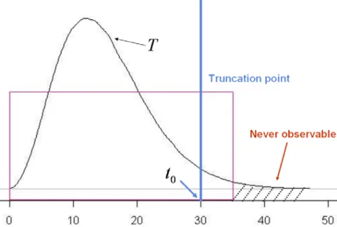
(21) 4.1.A The pairwise order indicator as the chosen response Cheng et al. (1995), suggested to use. I (X i ≥ X j , δ j = 1) G 2 (X j ). as the proxy of I (Ti ≥ T j ) .. Notice that. [. ]. [[ = E [I (T. E I (X i ≥ X j , δ j = 1) = E E Ti ≥ T j , C i ≥ T j , C j ≥ T j | Ti , T j i. ]. ≥ T j )G 2 (T ) .. ]]. This implies that. E[. I (X i ≥ X j , δ j = 1) ] = E[ I (Ti ≥ T j )], G 2 (X j ). if the denominator is not zero. See Appendix 2 for the details. The estimating equation in (3.1) can be modified as ⎛ ⎜ δ j I (X i ≥ X j ) T × − ξ Z ij η W ( Z η ) Z ⎜ ∑∑ ij ij 2 ^ i =1 i ≠ j ⎜ G (X ) j ⎝ n. (. T. ⎞ ⎟ ⎟ = 0, ⎟ ⎠. ). (4.2). ^. where G (.) is the Kaplan-Meier estimator Pr (C ≥ t ) . Despite its simplicity and convenience, the weighting approach has a series drawback. First of all, equation (4.2) produces (asymptotically) unbiased result only if the censoring support lies within the support of T . Specifically define τ c = sup{t : G (t ) > 0} and t. τ T = sup{t : Pr (T > t ) > 0} . The validity of (4.2) requires τ T ≤ τ c which eliminate the situation t. G(Ti ) = 0 . However, this assumption rarely holds in practice since the study period is often limited which makes τ T > τ c . This situation is developed in Figure (4.1).. 13.

(22) Figure 4.1 Problem for the weighting technique. To overcome this problem, Fine, Ying and Wei (1998) suggested to impose a truncation point t 0 (Figure 4.2) such that. I (min( X i ,t 0 ) ≥ X j , δ j = 1) G 2 (X j ). ,. where G (t 0 ) > 0 and t 0 is a prespecified constant satisfying.. Figure 4.2 Imposing a truncation point to overcome the problem. The corresponding expected value for the adjusted response is given by. 14.

(23) ξ ij * = E[. δ j I (min( X i ,t 0 ) ≥ X j ). ] = ξ ij (η ) − Pr (X i ≥ X j ≥ t 0 ). G2 (X j ). = E[ I (T j ≤ t 0 ) I (Ti ≥ T j )]. =∫. h(t0 ). −∞. T. {1 − Fε (t + Z ij η)}dFε (t ),. (4.3). which is a function of η and h(t 0 ) . See Appendix 3 for the details. Furthermore instead of using the first moment condition, Fine et al. (1998) proposed to use the least square principle by minimizing the objective function: 2. ⎛ ⎞ n ⎜ δ j I (min( X i , t 0 ) ≥ X j ) ⎟ * T ( ) × − η ξ η W Z ( ) ⎜ ⎟ , ∑∑ ij ij ^ 2 i =1 i ≠ j ⎜ ⎟ G (X j ) ⎝ ⎠ which leads to the estimating equation ⎛ ⎞ ⎜ δ j I (min( X i , t 0 ) ≥ X j ) ⎟ * ( ) − W ( Z ij η )ξ ij (η ) × ⎜ ξ η ⎟ = 0. ∑∑ ij ^ 2 i =1 i ≠ j ⎜ ⎟ G (X j ) ⎝ ⎠ n. '. T. For estimating h(t 0 ) , they also proposed another estimating function. Subramanian (2004) proposed a different way of modifying equation (3.1). The idea of Subramanian is to replace the original response I (Ti ≥ T j ) by an estimator of its nonparametric estimation. However, this method assumes that the covariate Z takes discrete values.. E (I (T. i. ∞. ≥ T )|Z ,Z ) = Pr (T j. i. j. i. ≥ T j|Z i ,Z j. ) = ∫ S (t|Z )dF (t|Z ).. i. i. 0. The Kaplan-Meier estimator can be applied to estimate S (t|Z ) such n. ^. S(t | Z) = ∏ {1u ≤t. ∑ I(X i =1. i. = u,δi = 1, Z i = z) }.. n. ∑ I(X i =1. i. ≥ u, Z i = z). Therefore, Subramanian develop its estimating equation,. 15.

(24) (. ^ ⎛∞ ^ T ⎜ ( ) (t|Z i ) − ξ Z ij Tη W ( Z η ) Z S t|Z d F × ∑∑ ij ij i ∫ ⎜ i≠ j ⎝0 ^. )⎞⎟⎟ = 0.. (4.4). ⎠. ∞. where S (t|Z i ) is the K-M estimation and ξ (t ) = ∫ {1-Fε (t + s )}dFε (s ) . But, t This method is -∞. also vulnerable to the tail problem since the Kaplan-Meier estimator can not catch the tail information either if τ T > τ c . Therefore, Subramanian used the same technique, imposing the truncation point t 0 , to develop the modified estimating equation, ^ ⎛ h (t 0 ) ^ T U s (η ) = ∑∑ W ( Z ij η ) Z ij × ⎜ ∫ S (t|Z i )d F (t|Z i ) − ξ * Z ij η ⎜ i≠ j ⎝ 0. (. T. )⎞⎟⎟ = 0. ⎠. 4.1.B The at-risk process as the chosen response Recall 3.1.B, Cai, Wei and Wilcox (2000) suggested to use Y (t ) as the response. Its expected value under the model is S (t | Z ) = φ -1 (h (t ) + Z T η ) . Under right censoring data, the corresponding response variable is I ( X i ≥ t ) . Thus, we can derived the expectation:. E [I ( X i ≥ t )] = Pr (Ti ≥ t , Ci > Ti ) = ϕ −1{h(t ) + Z i η}G (t ) . T. Cai et al. modify the equation (3.2a) as n. ∑[I (X i =1. T. i. ^. ≥ t ) − ϕ −1{h(t ) + Z i η }G (t )] = 0, t ∈ (τ a ,τ b ) .. (4.5a). Note that (4.5) provides a set of equations for t being the observed values of Ti (i = 1,..., n ) . If η is one-dimensional, there are n + 1 unknown parameters in (4.5). Therefore we need one more equation. Cai et al. (2000) suggested the following equation n. τb. i =1. a. ∑ ∫τ. ^. Z i [ I (Ti ≥ t ) − ϕ −1{h(t ) + Z i η } G (t )]dt = 0 , T. (4.5b). where (τ a ,τ b ) is a re-specified range that contains enough data information. Solve equations (4.5a) and (4.5b) iteratively. The following numerical operation is the same as 3.1.B we 16.

(25) mentioned.. 4.1.C The counting process as the chosen response With censoring data structure, using the estimating equation based on counting process is easily modifying. We would not change the formation we mentioned in 3.1.B. That is to say, it is very generalized method in constructing the estimating equation in linear transformation model.. 4.2 Likelihood Inference The likelihood function in (3.6) can be extended to the censoring situation as follows: δi. ⎡ ∂ϕ −1 (η, z i , h (t )) ⎤ 1−δ −∏⎢ |t = xi ⎥ ϕ −1 (η, z i , h ( xi )) i . ∂t i =1 ⎣ ⎦ n. Since direct maximization is impossible, how to handle the nuisance function h (.) is the key.. 4.2.1 Partial Likelihood – Cox model Here we illustrate the way Cox (1972, 1975) used to handle the nuisance baseline hazard function λ0 (t ) under the model λ (t|Z ) = λ0 (t ) × exp (Z T η ) . At time t , the probability that the failure event is for patient i given the risk set information is. ( ). ). ( ). ). I ( X i = t , δ i = 1) λ0 (t ) × exp Z i η I ( X i = t , δ i = 1) exp Z i η = , T T ∑ λ0 (t ) × exp Z j η ∑ exp Z j η j∈R (t ). (. T. j∈R (t ). (. T. where R (t ) = {j : X j ≥ t , δ j =1 } is the risk set at time at time t . The important point is that the same λ0 (t ) appears in both the numerator and denominator and hence gets cancelled out. Thus the above conditional probability is only the function of η . The so-called partial likelihood can be written as. (. ⎧ n T ⎪ ∑ I ( X i = u,δi = 1) × exp Z i η ⎪ i =1 ⎨ ∏ n all failture points u ⎪ ∑ I (X j ≥ u ) × exp Z j T η ⎪⎩ j =1. (. ). )⎫⎪⎪. ⎬, ⎪ ⎪⎭. (4.6). Since λ0 (t ) disappears, maximization of (4.6) becomes easy. The corresponding score function 17.

(26) can be written as. ∑ I (X n. D. U (η ) = ∑ [ Z (i )i =1. j. j =1 n. ∑ I (X j =1. (. ≥ t (i ) )Z j × exp Z j η j. (. T. ≥ t (i ) ) × exp Z j η T. ). ) ],. n. where t (i ) is the order values of X j with δ j = 1 for j = 1,..., n and D = ∑ δ j is the total j =1. number of observed failure events.. 4.2.2 Conditional Profile Likelihood The amazing cancellation for the Cox partial likelihood does not happen to the more general class of transformation models. Therefore if the likelihood approach is pursued, the nuisance function has to be dealt with directly. For the general transformation model in (1.4), Pr (T > t|Z = z ) = Pr{ε > h(t ) + z T η} = ϕ -1 (h(t ) + Z T η ), Chen, H. Y. (2001) proposed a likelihood approach for the case-cohort study, the covariate Z has an unknown distribution π (z ) = Pr (Z ≤ z ) , which is a more complex data structure than that considered in the thesis. Now we organize his method based on our data structure. By writing the full likelihood as. ∏ [ f (x ) n. η. i =1. i. δi. S η ( xi ). 1-δi. ]. ⎡⎛ ∂ ⎤ ⎞ = ∏ ⎢⎜ - ϕ -1 {η,Z i ,h( xi )}⎟dπ ( z )⎥ ⎠ i =1 ⎣⎝ ∂t ⎦ n. δi. [ϕ. -1. {η,Z i ,h(xi )}dπ (z )] 1-δ , i. Chen suggested to express the function in terms of η and the marginal survival distribution of T , such that. (. ). R (t ) = Pr (T ≥ t ) = ∫ ϕ -1 h(t ) + Z T η dπ (z ) ,. (4.7). where π (z ) = Pr (Z ≤ z ) is the distribution function of Z . The motivation of the above transformation is that R (t ) can be estimated by the Kaplan-Meier estimator 18.

(27) n. Rˆ (t ) = ∏ {1 − u ≤t. ∑ I(X. i. = t , δ i = 1). i =1. }.. n. ∑ I(X. i. ≥ t). i =1. This implies that R (t ) , as a complicated function of η , h (.) and H (.) , can be estimated. n. The distribution function π (.) can also be estimated explicitly by πˆ ( z ) = ∑ I ( Z i ≤ z ) / n . i =1. Based on (4.7), one can derive the relationship between h (t ) and {R ( t ), η , H (.)} by inverse transformation. Denote v = v{η, π , R} as the transformation. The technical issue is not the focus of the thesis so that we do not state the details. Finally, after the transformation, η can be estimated by maximizing the following profile likelihood function:. {. (. )}. δ. i ∂ -1 ⎡ ⎤ ˆ 1-δi ˆ ( ) ( ) π φ η,z ,v η, z , R x n ⎢ i i i ⎥ ⎡ φ -1 η,z i ,v η,πˆ ( z i ),Rˆ ( xi ) ⎤ ∂ ⎢ ⎥ ⎢ ⎥ . ∏ ˆ (x ) ∂ -1 R ⎢ i =1 ⎢ ˆ ⎥ i ⎣ ⎦⎥ φ η,z i ,v η,πˆ (z i ),R( xi ) dπˆ ( z i ) ⎣⎢ ∫ ∂ ⎦⎥. {. (. )}. {. (. )}. This approach is very complicated and difficult to implement. The validity of the resulting estimator depends on whether the suggested transformation has to be a one-to-one mapping.. 19.

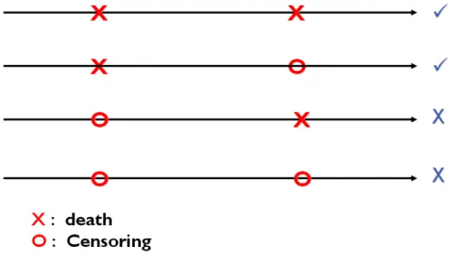
(28) Chapter 5. New Proposed Method. Under pairwise method, we propose to directly modify the whole equation:. ∑∑ W ( Z. T ij. (. (. )). η ) Z ij × I (Ti ≥ T j ) − ξ Z ij Tη = 0 .. i≠ j. Specifically we only select pairs with the value of I (Ti ≥ T j ) being exactly known. To illustrate the idea, we can examine the two cases. Case 1: If I (X i ≥ X j , δ j = 1) , we know that X j = T j and I (Ti ≥ T j ) = 1 . Case 2: If I (X i ≥ X j , δ j = 0 ) , we have T j > X j and Ti > X j but the order of (Ti , T j ). is uncertain. The following figure depicts the possible order relationships for a pair subject to censoring.. Figure 5.1: The order relationship for a pair subject to censoring. Define. Δ ij = I((δ i = 1, δ j = 1) ∪ (X i > X j , δ i = 0, δ j = 1) ∪ (X i < X j , δ i = 1, δ j = 0 )). as. the. orderable indicator which corresponds to I (X i ≥ X j , δ j = 1) or I (X j ≥ X i , δ i = 1) . The corresponding estimating function is given by. (. ). U new (η ) = ∑∑ W Z ij η × Z ij × Δ ij × (I (X i ≥ X j ) − ξ (Z ij η )) . i≠ j. T. (5.1). The proposed estimator is obtained by solving U new (η ) = 0 . In Appendix 4, unbiasness of the 20.

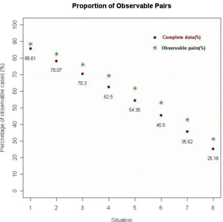
(29) estimator is proved. We may study the proportion of the data that has been used in estimation. Define ⎛n⎞ p1 = ∑ I (δ i = 1) / n and p2 = ∑∑ I ( Δ ij = 1) / ⎜⎜ ⎟⎟ . By changing the censoring proportions, i =1 i =1 j ≠i ⎝2⎠ n. n. we see that 1 > p2 > p1 . The new propose method uses p2 of the data. However all the rest estimators use almost 100% of the data. The major advantage of our method is that there is no need to estimator other nuisance parameters and remains unbiasness even under censoring. The disadvantage is that 1 − p2 of the data is deleted. The loss of efficiency under heady censoring is expected.. Figure 5.2: The observable proportion: Original data vs. Paired data. In addition, the new method losses too many data in using the comparable indicator Δ ij and causes the inefficient outcome. Thus, we want to improve this estimating equation to avoid missing too many information. We consider the following situation in Figure 5.3. Using comparable indicator Δ ij , we drop all the data in this situation. We use imputation technique 21.

(30) and Kaplan-Meier estimator to modify the original equation.. Figure 5.3: (X i > X j , δ i = 1, δ j = 0 ) ∪ (X j > X i , δ j = 1, δ i = 0 ). We imposed new comparable indicator Δ ij * = I (X i > X j , δ i = 1, δ j = 0) and imputation technique to renew our estimating equation:. (. ). ∧ ⎧ ⎤⎫ ⎡⎛ ∧ * T ⎞ ( ) ( ) ( ) W Z η Z I X X ξ Z η 1 S X / S × × Δ × ≥ − + Δ × − Z Z j ( X j )⎟ − ξ (Z ij η ) ⎬ , ⎜ ⎨ i ∑∑ ij ij ij i j ij ij i ⎥ ⎢ ⎠ ⎦⎭ ⎣⎝ i≠ j ⎩. [. ]. ∧. where S ( X ) is the Kaplan-Meier estimator.. 22.

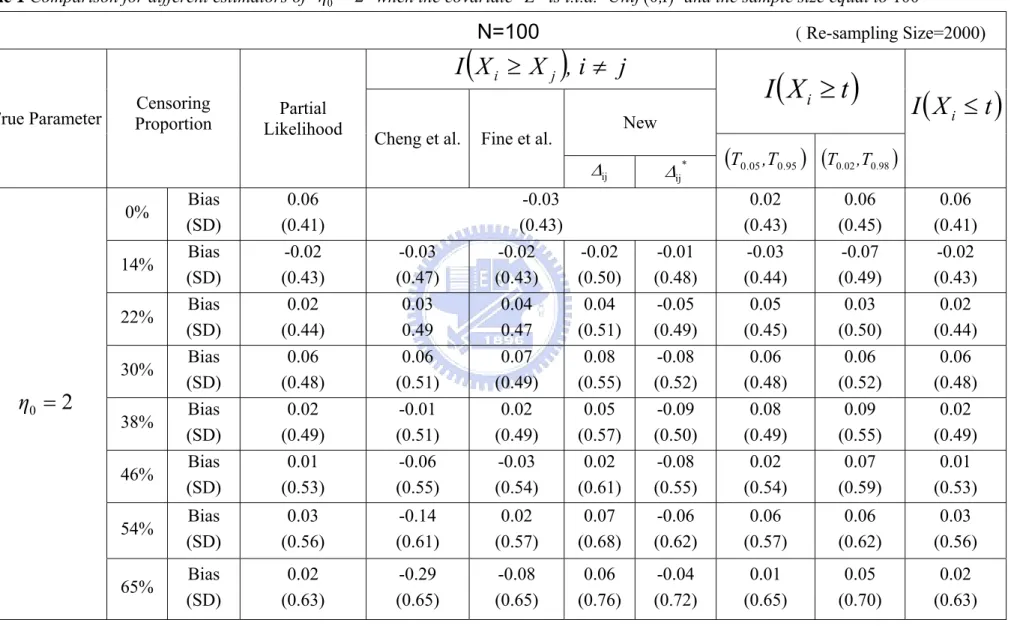
(31) Chapter 6. Simulation. We conduct Monte Carlo simulations to examine the finite-sample performances of the methods in the thesis. Based on the model, h(T ) = -η T Z + ε , we consider its special case, namely the Cox proportional hazard models. These Cox model is the most popular in practical applications. The covariate Z follows Bernoulli(0.5) or U (0,1) . The censoring variable C is generated from uniform distributions. Two sample sizes are considered, namely n =100 or 250. For each setting, 2000 replications are run. The average bias and standard deviation of each method are reported.. 6.1 Cox proportional hazard model The error term follows the extreme value distribution with Fε (s ) = 1- exp(- exp(s )) . It follows that ∞. ξ (s ) = ∫ {1-F (t + s )}dF (t ) = -∞. 1 1 + exp(s ). and. (. (e e p 1-e-e ξ ( p, s | t 0 ) = e p + es *. h ( t0 ) -p-s. p. +es. ). ).. The latter is used in the work of Fine et al. (1998) which requires specifying the truncation point related to the range of integration. Here we choose t 0 = 0.5 . For the estimating function proposed by Cai et al. (2000), we set (τ a , τ b ) to be (T0 .05 ,T0 .95 ) and (T0 .02 ,T0 .98 ) .. 6.2 Discussion Besides the results of the moment-based methods, we also report the result of the Cox partial likelihood estimator. Recall that the methods discussed in thesis are suitable of all members in the model class but the partial likelihood estimator is developed only for the Cox model. In absence of censoring, the results produced by the pairwise comparison approach are 23.

(32) similar to those of the partial likelihood method. However the weighting adjustment by Cheng et al. (1995) is problematic when censoring becomes heavier due to the tail problem mentioned earlier. The modification by Fine et al. (1998) by adding a truncation point successfully fixes the tail problem. Subramanian (2004) suggest using the nonparametric estimation to replace the pairwise indicator when data is censoring. However, the method of Subramanian is suitable under one important assumptation, the covariates Z follows discrete distribution. Our method uses the idea of choosing only comparable pairs to develop the unbiased estimating equation. However, we find that method losses too many data when censoring is heavy, the performance of estimation is inefficient (variance is relatively large). Thus, we use imputation technique to add a new comparable indicator Δij to avoid losing too many data. In numerical outcome, we *. find that the equation imposing new comparable indicator Δij is more efficient. *. The approach by Cai et al. (2000) used at-risk process approach which requires specification of (τ a ,τ b ) and we see that this choice affects the result. If the range is set too wide including the extreme value, the variation of the estimator gets larger. How to choose the suitable (τ a ,τ b ) becomes the biggest problem in this method. The counting process approach is the ideal method in the linear transformation models. In addition, we prove that counting process approach is equal to the specific method, Cox partial likelihood (1975), under Cox PH model in appendix 5. Because counting process approach uses the advantage of martingale, we find the numerical results of Chen et al.’s (2002) in below tables is more efficient than other unified methods. In theory, Chen’s method also has good properties and generalization.. 24.

(33) Table 1 Comparison for different estimators of η0 = 2 when the covariate Z is i.i.d. Unif (0,1) and the sample size equal to 100. N=100. ( Re-sampling Size=2000). I (X i ≥ X j ), i ≠ j True Parameter. Censoring Proportion. Partial Likelihood. Cheng et al.. New. Fine et al.. Δij Bias (SD) Bias (SD) Bias (SD) Bias (SD) Bias (SD) Bias (SD). 0.06 (0.41) -0.02 (0.43) 0.02 (0.44) 0.06 (0.48) 0.02 (0.49) 0.01 (0.53). 54%. Bias (SD). 65%. Bias (SD). 0% 14% 22% 30%. η0 = 2. 38% 46%. -0.03 (0.47) 0.03 0.49 0.06 (0.51) -0.01 (0.51) -0.06 (0.55). -0.03 (0.43) -0.02 (0.43) 0.04 0.47 0.07 (0.49) 0.02 (0.49) -0.03 (0.54). -0.02 (0.50) 0.04 (0.51) 0.08 (0.55) 0.05 (0.57) 0.02 (0.61). 0.03 (0.56). -0.14 (0.61). 0.02 (0.57). 0.02 (0.63). -0.29 (0.65). -0.08 (0.65). 25. I (X i ≥ t ) Δij *. I (X i ≤ t ). (T0 .05 ,T0 .95 ) (T0.02 ,T0.98 ). -0.01 (0.48) -0.05 (0.49) -0.08 (0.52) -0.09 (0.50) -0.08 (0.55). 0.02 (0.43) -0.03 (0.44) 0.05 (0.45) 0.06 (0.48) 0.08 (0.49) 0.02 (0.54). 0.06 (0.45) -0.07 (0.49) 0.03 (0.50) 0.06 (0.52) 0.09 (0.55) 0.07 (0.59). 0.06 (0.41) -0.02 (0.43) 0.02 (0.44) 0.06 (0.48) 0.02 (0.49) 0.01 (0.53). 0.07 (0.68). -0.06 (0.62). 0.06 (0.57). 0.06 (0.62). 0.03 (0.56). 0.06 (0.76). -0.04 (0.72). 0.01 (0.65). 0.05 (0.70). 0.02 (0.63).

(34) Table 2 Comparison for different estimators of η0 = 2 when the covariate Z is i.i.d. Unif (0,1) and the sample size equal to 250. N=250. ( Re-sampling Size=2000). I (X i ≥ X j ), i ≠ j True Parameter. Censoring Proportion. Partial Likelihood. New Cheng et al.. Fine et al.. Δij Bias (SD) Bias (SD) Bias (SD) Bias (SD) Bias (SD) Bias (SD). 0.01 (0.25) 0.00 (0.27) 0.01 (0.25) 0.02 (0.28) 0.02 (0.28) 0.02 (0.30). 54%. Bias (SD). 65%. Bias (SD). 0% 14% 22% 30%. η0 = 2. 38% 46%. I (X i ≥ t ). 0.00 (0.31) 0.01 (0.29) 0.01 (0.32) -0.01 (0.32) -0.04 (0.34). 0.01 (0.25) 0.00 (0.27) 0.01 (0.26) 0.02 (0.29) 0.01 (0.31) 0.02 (0.33). 0.00 (0.32) 0.01 (0.31) 0.03 (0.34) 0.03 (0.35) 0.03 (0.38). 0.01 (0.35). -0.13 (0.38). 0.00 (0.37). 0.00 (0.37). -0.33 (0.40). -0.01 (0.40). 26. Δij *. I (X i ≤ t ). (T0 .05 ,T0.95 ) (T0.02 ,T0.98 ). -0.05 (0.30) -0.07 (0.29) -0.08 (0.29) -0.09 (0.31) -0.08 (0.33). 0.02 (0.26) 0.01 (0.29) 0.02 (0.29) 0.02 (0.30) 0.01 (0.33) -0.02 (0.34). 0.04 (0.30) 0.04 (0.31) 0.05 (0.33) 0.06 (0.35) 0.04 (0.36) 0.05 (0.38). 0.01 (0.25) 0.00 (0.27) 0.01 (0.25) 0.02 (0.28) 0.02 (0.28) 0.02 (0.30). 0.02 (0.42). -0.06 (0.36). -0.01 (0.38). 0.08 (0.40). 0.01 (0.35). 0.02 (0.46). -0.04 (0.43). 0.03 (0.40). 0.06 (0.42). 0.00 (0.37).

(35) Table 3 Comparison for different estimators of η0 = 2 when the covariate Z is i.i.d. Ber(0.5) and the sample size equal to 100. N=100. ( Re-sampling Size=2000). I (X i ≥ X j ), i ≠ j True Parameter. Censoring Proportion. Cheng et al. Fine et al. Subramanian. Bias (SD) Bias (SD) Bias (SD) Bias (SD) Bias (SD) Bias (SD). 0.04 (0.30) 0.03 (0.30) 0.03 (0.31) 0.04 (0.33) 0.05 (0.34) 0.05 (0.40). 0.05 (0.36) 0.04 (0.36) 0.06 (0.40) 0.06 (0.39) 0.03 (0.46). 54%. Bias (SD). 0.06 (0.42). 65%. Bias (SD). 0.08 (0.46). 0% 14% 22% 30%. η0 = 2. Partial Likelihood. 38% 46%. I (X i ≥ t ) New. Δij. 0.05 (0.32) 0.04 (0.33) 0.06 (0.35) 0.06 (0.35) 0.06 (0.41). 0.04 (0.34) 0.05 (0.35) 0.04 (0.37) 0.02 (0.39) 0.03 (0.40) 0.04 (0.46). 0.05 (0.36) 0.05 (0.37) 0.06 (0.41) 0.09 (0.42) 0.08 (0.49). 0.12 (0.46). 0.08 (0.43). 0.03 (0.47). -0.35 (0.51). -0.09 (0.46). -0.08 (0.52). 27. Δij *. I (X i ≤ t ). (T0 .05 ,T0.95 ) (T0.02 ,T0.98 ). 0.00 (0.35) -0.03 (0.34) -0.04 (0.35) -0.06 (0.36) -0.06 (0.40). 0.06 (0.30) 0.05 (0.32) 0.02 (0.34) 0.00 (0.36) 0.01 (0.37) 0.02 (0.42). 0.04 (0.32) -0.05 (0.35) 0.06 (0.36) 0.08 (0.39) -0.05 (0.41) 0.04 (0.48). 0.04 (0.30) 0.03 (0.30) 0.03 (0.31) 0.04 (0.33) 0.05 (0.34) 0.05 (0.40). 0.07 (0.48). -0.07 (0.41). 0.08 (0.43). -0.06 (0.51). 0.06 (0.42). 0.07 (0.55). 0.07 (0.45). 0.04 (0.49). 0.08 (0.53). 0.08 (0.46).

(36) Table 4 Comparison for different estimators of η0 = 2 when the covariate Z is i.i.d. Ber(0.5) and the sample size equal to 250. N=250. ( Re-sampling Size=2000). I (X i ≥ X j ), i ≠ j True Parameter. Censoring Proportion. Cheng et al. Fine et al. Subramanian. Bias (SD) Bias (SD) Bias (SD) Bias (SD) Bias (SD) Bias (SD). 0.00 (0.17) 0.02 (0.19) 0.03 (0.18) 0.01 (0.20) 0.01 (0.21) 0.01 (0.23). 0.03 (0.22) 0.02 (0.21) 0.02 (0.24) 0.01 (0.23) -0.02 (0.27). 54%. Bias (SD). 0.03 (0.26). 65%. Bias (SD). 0.03 (0.30). 0% 14% 22% 30%. η0 = 2. Partial Likelihood. 38% 46%. I (X i ≥ t ) New. Δij. 0.03 (0.19) 0.03 (0.19) 0.02 (0.21) 0.02 (0.20) 0.02 (0.23). 0.02 (0.20) 0.05 (0.20) -0.03 (0.21) -0.02 (0.24) 0.05 (0.22) 0.02 (0.28). 0.03 (0.23) 0.03 (0.22) 0.02 (0.25) 0.02 (0.24) 0.03 (0.28). -0.08 (0.34). -0.02 (0.31). 0.02 (0.32). -0.33 (0.33). -0.07 (0.29). 0.08 (0.33). 28. Δij *. I (X i ≤ t ). (T0 .05 ,T0.95 ) (T0.02 ,T0.98 ). -0.03 (0.19) -0.06 (0.21) -0.06 (0.21) -0.08 (0.22) -0.09 (0.26). 0.02 (0.19) 0.03 (0.22) -0.05 (0.22) 0.02 (0.23) 0.01 (0.24) -0.01 (0.26). 0.04 (0.21) 0.05 (0.23) 0.07 (0.24) 0.06 (0.25) -0.08 (0.28) 0.06 (0.30). 0.00 (0.17) 0.02 (0.19) 0.03 (0.18) 0.01 (0.20) 0.01 (0.21) 0.01 (0.23). 0.05 (0.31). -0.08 (0.25). 0.05 (0.29). -0.05 (0.32). 0.03 (0.26). 0.04 (0.35). -0.08 (0.30). 0.04 (0.33). 0.06 (0.35). 0.03 (0.30).

(37) Chapter 7. Concluding Remarks. In this thesis, we consider semiparametric inference for linear transformation models which form a general class of regression models. We review existing literature under the classical framework of estimation theory. Specifically the method of moment and likelihood method are the two most important principles for parameter estimation. Here we see that how these approaches are adapted to the semi-parametric structure. The method of moment usually yields simpler solutions than the likelihood method in presence of high-dimensional nuisance parameter, namely h (.) , in our problem. Another focus of thesis is to review how censoring is handled in an estimation procedure. The weight approach is appealing due to its simplicity. However we have seen that the suggested weight, in terms of the reciprocal of a Kaplan-Meier estimator, is sensitive to the tail estimation. When the censoring support lies within the support of the true lifetime, the weighting method can lead to bias solution. Nevertheless, Fine et al. (1998) proposed to further truncate the tail area to fix this problem. The method utilizing the martingale theory proposed by Chen, Jin and Ying (2002), is appealing in presence of censoring. First of all, it can be easily modified for censored data without estimation of G (.) . It does not need to select the range of integration as Cai et al. (2000) did for (τ a ,τ b ) since the expectation conditional on Ft − can update the most recent information and hence flexible. The likelihood approach is useful for the Cox model since the nuisance function gets cancelled out in estimating the conditional hazard. However likelihood inference becomes very complicated under the more general model setting.. 29.

(38) Appendix Appendix 1: Prove ξ (s ) = Pr (ε i − ε j ≥ s ) = ∫ {1 − Fε (t + s )}dFε (t ) ∞. −∞. Let V = ε i − ε j and. iid. ε ~ f ε (ε ). By convolution, we can find the following result:. f T (t ) = ∫ f εi ,ε j (v + ε j ,ε j ) dε j = ∫ f ε (v + ε j )× f ε (ε j ) dε = ∫ f ε (v + ε j ) dFε (ε j ). ∞. ∞. ∞. -∞. -∞. -∞. Thus,. ξ (s)= Pr( ε i − ε j ≥ s ) =. ∞. ∞. s. -∞. ∫ ∫ =∫. ∞. ∫. ∞. -∞ s. f ε (v + ε j ) dFε (ε j ) dv f ε (v + ε j ) dv dFε (ε j ). s ∞ = ∫ 1-⎛⎜ ∫ f ε (s + ε j )dv ⎞⎟ dFε (ε j ) -∞ ⎝ -∞ ⎠. = ∫ 1-Fε (ε j + s ) dFε (ε j ) ∞. -∞ ∞. = ∫ {1 − F (t + s )} dF (t ) , −∞. where F (s ) = Pr(ε ≤ s ) .. Appendix 2: Unbiased property for Cheng’s. Recall that Cheng’s estimating equation under right censoring: ⎛ ⎜ δ j I (X i ≥ X j ) T − ξ Z ij η U (η ) = ∑∑ W ( Z ij η ) Z ij × ⎜ 2 i =1 i ≠ j ⎜ ⎝ G (X j ) n. (. T. ⎞ ⎟ ⎟, ⎟ ⎠. ). ∞. where ξ (s ) = ∫ {1-Fε (t + s )}dFε (s ) . -∞. Now, we want to show that equation (A-1) is unbiased. That is to say, we will prove. 30. (A-1).

(39) E[. δ j I (X i ≥ X j ) G (X j ) 2. (. ). | Z i ,Z j ] = ξ Z ij η . T. We use the conditional double expectation technique in the following: E[. δ j I (X i ≥ X j ) G 2 (X j ). | Z i ,Z j ] = E[. I (C j ≥ T j ) I ( X i ≥ X j ) G2 (X j ). = E[ E[ = E[ E[ = E[. I (min(C j ,X i ) ≥ T j ) G 2 (T j ). |Z i ,Z j ] |Z i ,Z j ,T j ]]. I (Ti ≥ T j ) I (min(C i ,C j ) ≥ T j ) G 2 (T j ). Pr( min(C i ,C j ) ≥ T j ) G 2 (T j ). |Z i ,Z j ,T j ]]. E[ I (Ti ≥ T j )|Z i ,Z j ,T j ]]. = E[ E[ I (Ti ≥ T j )|Z i ,Z j ,T j ]] = E[ I (Ti ≥ T j )|Z i ,Z j ] = Pr( h(Ti ) ≥ h(T j ) | Z i , Z j ). = Pr(ε i − ε j ≥ Z ij η | Z i , Z j ) T. (. ). = ξ Z ij η . T. Appendix 3: Unbiased property for Fine’s. Fine et al. added a truncation point t 0 to overcome the biased problem of Cheng et al.’s estimating equation. We recall Fine’s estimating equation: ⎛ ⎞ ⎜ δ j I (min( X i , t 0 ) ≥ X j ) ⎟ * U f (η ) = ∑∑ W ( Z ij η )ξ ij (η ) × ⎜ − ξ ij (η )⎟ , 2 i =1 i ≠ j ⎜ ⎟ G (X j ) ⎝ ⎠ n. where ξ * ij (η 0 ) = ∫. h(t0 ). −∞. T. '. T. {1 − Fε (t + Z ij η0 )}dFε (t ) .. Now, we want to prove equation (A-2) is unbiased. Thus, we will show that. 31. (A-2).

(40) ⎡ ⎤ ⎢ δ j I (min( X i , t 0 ) ≥ X j ) ⎥ E⎢ |Z i ,Z j , t o ⎥ = ξ * ij (η ) . 2 ⎢ ⎥ G (X j ) ⎣ ⎦. Again, we take advantage of the conditional double expectation technique in our procedure: E[. δ j I (min( X i ,t 0 ) ≥ X j ). I (C i ≥ T j ) I ( X i ≥ X j ) I ( X j ≤ t 0 ). G2(X j ). G 2(X j ). |Z i ,Z j , t o ] = E[. = E[ E[ = E[ E[ = E[. I (min( X i ,C i ) ≥ T j ) I (T j ≤ t 0 ) G2 (X j ). |Z i ,Z j , t o ]. |Z i ,Z j ,t o ,T j ]]. I (Ti ≥ T j ) I (min(C i ,C j ) ≥ T j ) I (T j ≤ t 0 ) G 2 (T j ). Pr (min(C i ,C i ) ≥ T j ) G 2 (T j ). |Z i ,Z j ,t o ,T j ]]. I (T j ≤ t 0 ) E[ I (Ti ≥ T j )|Z i ,Z j ,t o ,T j ]. = E[ I (T j ≤ t 0 ) E[ I (Ti ≥ T j )|Z i ,Z j ,to ,T j ]] = E[ I (T j ≤ t 0 ) I (Ti ≥ T j )|Z i ,Z j ,t o ] = Pr(T j ≤ t0 , Ti ≥ T j|Z i ,Z j t o ) = Pr(Ti ≥ T j|Z i ,Z j )-Pr(T j ≥ t0 , Ti ≥ T j|Z i ,Z j to ) = Pr( h(Ti ) ≥ h(T j )|Z i ,Z j ) - Pr(Ti ≥ T j ≥ to|Z i ,Z j ,t o ) = Pr( h(Ti ) ≥ h(T j )|Z i ,Z j )- Pr( h(Ti ) ≥ h(T j ) ≥ h(to )|Z i ,Z j ,t o ). =∫. h(t0 ). −∞. T. {1 − Fε (t + Z ij η)}dFε (t ). = ξ * ij (η ) .. Appendix 4: Unbiased property for New proposed method. We take the observing pairs to be our main idea to develop our simple method. Therefore, we use an indicated function I((Ti ∧ T j ) < (C i ∧ C j )) to construct our estimating equation. Now, we would show that new estimating equation we proposed is unbiased. For convenience, we let I((Ti ∧ T j ) < (C i ∧ C j )) = Δ ij , and recall our simple estimating equation:. 32.

(41) (. ). U new (η ) = ∑∑ W Z ij η × ξ ' (Z ij η )× Δij × (I (X i ≥ X j ) − ξ (Z ij η )) . i≠ j. T. [. ]. In the beginning, we want to find E I(X i ≥ X j ) − Pr (Ti ≥ T j ) | (Ti ∧ T j ) < (C i ∧ C j ) . Thus, we use two cases to help us analyze the problem: Given (Ti ∧ T j ) = Ti and (Ti ∧ T j ) < (Ci ∧ C j ). 1.. Then Ti is the smallest of Ti , T j , C i and C j Therefore, we can get T j ^ C j ≥ Ti => X j ≥ Ti Given (Ti ∧ T j ) = T j and (Ti ∧ T j ) < (Ci ∧ C j ). 2.. Then T j is the smallest of Ti , T j , C i and C j Therefore, we can get Ti ^ C i ≥ T j => X i ≥ T j Then, we can make some inference based on above information:. [. ]. E I(X i ≥ X j ) − Pr (Ti ≥ T j ) | (Ti ∧ T j ) < (C i ∧ C j ). [. ]. [. ]. = E I(X i ≥ X j ) − Pr (Ti ≥ T j ) | (Ti ∧ T j ) < (C i ∧ C j ), (Ti ∧ T j ) = Ti × Pr ((Ti ∧ T j ) = Ti ) + E I(X i ≥ X j ) − Pr (Ti ≥ T j ) | (Ti ∧ T j ) < (C i ∧ C j ), (Ti ∧ T j ) = T j × Pr ((Ti ∧ T j ) = T j ) = Pr (Ti ≥ X j | (Ti ∧ T j ) < (C i ∧ C j ), (Ti ∧ T j ) = Ti )× Pr ((Ti ∧ T j ) = Ti ) + Pr (X i ≥ T j | (Ti ∧ T j ) < (C i ∧ C j ), (Ti ∧ T j ) = T j )× Pr ((Ti ∧ T j ) = T j ). = (0-0) × Pr (Ti ∧ T j = Ti ) +(1-1) × Pr (Ti ∧ T j = T j ) =0 Appendix 5: Chen et al. (2002) is equal to partial likelihood method under Cox model. Consider the special case of the Cox model, in which λ (t ) = exp(t ) . We use this result. λ (t ) = exp(t ) , plug into equation (3.3). We can find the following result,. 33.

(42) n. ∑ dN (t ). [ ]=. de. h (t ). i =1. i. ∑ Y (t ) × exp(Z η) n. .. T. i. i =1. If we plug the result (3.5) in the martingale integral equation (3.4), we obtain. ∑ I (T. (. ≥ T(i ) )z j × exp z j η. n. D. U(η ) = ∑ [ Z (i )i =1. j =1. j. ∑ I (T n. j =1. j. (. T. ≥ T(i ) )× exp z j η T. ). ) ] =0,. which is precisely the Cox partial likelihood score equation.. Appendix 6: trend plot of new proposed method. 34.

(43) References [1] Andersen, Per Kragh, Borgan, Ornulf, Gill, Richard D.& Keiding, Niels (1997) Statistical Models Based on Counting Process. Springer Series in Statistics. [2] Buckley, Jonathan & James, Ian (1979). Linear Regression with Censored Data.. Biometrika , Vol. 66, No. 3., pp. 429-436. [3] Cai, T., Wei L. J., Wilcox, M. (2000). Semiparametric regression analysis for clustered failure time data. Biometrika , 87, 4, pp. 867-878. [4] Chen, H. Y.(2001). Fitting Semiparameteric Transformation Regression Models to Data form a Modified Case-Cohort Design. Biometrika , 88, 1, pp. 255-268. [5] Chen, K., Jin, Z. & Ying, Z. (2002). Semiparametric analysis of transformation models with censored data. Biometrika , 89, 3, pp. 659-668. [6] Cheng, S. C., Wei, L. J. & Ying, Z. (1995). Analysis of transformation models with censored data. Biometrika , 82, 4, pp. 835-45. [7] Cheng, S. C., Wei, L. J. & Ying, Z. (1997). Prediction of survival probabilities with semi-parametric transformation models. JASA , 92, pp. 227-76. [8] Cox, D. R. (1972). Regression models and life tables (with Discussion).. J. R. Statist. Soc. B 34, 187-220. [9] Cox, D. R. (1975). Partial likelihood. Biometrika 62, 269-76. [10] Fine, J. P., Ying, Z. & Wei, L. J. (1998). On the linear transformation model with censored data. Biometrika , 85, pp. 980-6. [11] Green, P.J. and Silverman, B.W. (1994) Nonparametic Regression and Generalized Linear Models. A roughness penalty approach. Monographs on Statistics and Applied. Probability 58 [12] Klein, J. P. and Moeschberger, M. L. (1997). Survival Analysis: Techniques for Censored and Truncated Data, Springer-Verlag, New York. 35.

(44) [13] Miller, R. & Halpern, J. (1982). Regression with censored data. Biometrika 69, 521-31. [14] Pettitt, A. N. (1984). Proportional odds model for survival data and estimates using ranks. Appl. Stat ist. 33, 169-75.. [15] Subramanian, S. (2003). Semiparametric transformation models and the missing information principle. Journal of Statistic al Plannin g and Infe rence 115 327 V 348. [16] Subramanian, S. (2004). A correction note on “Semiparametric transformation models and the missing information principle”. Journal of Statistic al Plannin g and Infe rence. 126 397 - 399 [17] Tsiatis, Anastasios A.(2006). Semiparametric Theory and Missing Data. Springer Series in Statistics. 36.

(45)