量子點在高壓下的發光效應和量子點模型建構

國立交通大學

物理研究所

碩 士 論 文

量子點在高壓下的發光效應和量子點模型

建構

Modeling and high pressure experiment of

CdSe/ZnS Colloidal QDs

研究生：邱奎霖

指導教授：褚德三

量子點在高壓下的發光效應和量子點模型建構

學生：邱奎霖 指導教授：褚德三

國立交通大學物理研究所

摘要

本論文主要是研究膠狀的複層量子點,核為 CdSe 外殼為 ZnS,在高壓下的發

光效應，實驗是量測量子點的Raman, PL, 和 life time 光譜。從這些光譜中我們

研究量子點能階隨壓力的變化、晶體結構隨壓力可能之改變，以及量子光學理論 對於這種介於原子和固體中間之尺度的量子點之適用程度。 從拉曼和PL 光譜中我們發現量子點也存在壓力所引起的相變點，但由於外層 ZnS 的保護，使得它的相變壓力比起塊材的相變壓力(3GPA)來的大，要到 7GPA 才會相變。而由於相變後PL 不存在也讓我們猜測相變後的內層 CdSe 是呈金屬 相，即如同塊材CdSe 相變後的 rocksalt 結構，由第一原理計算知道其導帶與價 帶重疊因而為金屬相。而從退壓拉曼我們發現當壓力又小於7GPA 時，CdSe LO 譜峰會重現但2LO 模卻消失，因此我們也猜測 CdSe 經過一次相變後就算壓力回 覆仍然不能回到之前的相；即這個相變是不可逆相變。而ZnS 的 LO 模加壓退 壓曲線幾乎重合,因此可知,此複層量子點的 ZnS 殼僅僅隨壓力而壓縮而未發生相 變。 我們也由PL 光譜佐以拉曼光譜來研究量子點能隙隨著壓力的變化。我們知 道量子點隨著加壓除了電子結構改變所引起的能階改變外，仍有電子-聲子的交 互作用能量(polaron 能量)的貢獻，而經由拉曼 CdSe 的 LO,2LO 模的 Grűneisen

參數顯示晶體的離子性會隨壓力降低，這會減低polaron 形成的能力，也會減低 電子-聲子的交互作用能量。故我們可以預期隨著加壓,量子點的 polaron 能量會 降低，所以再高壓時，能階曲線會呈現較為平滑的趨勢。我們也在第三章對這個 現象做一個簡單模型的討論。 至於量子點輻射的時間解析部分，我們結合量子光學中一個理想二能階原子 的輻射衰退率公式，和在塊材中加一個侷限位勢的量子點模型，並利用費米黃金 定律所解出之受激輻射衰退率公式。利用這兩種理論的結合來討論我們所作到的 life time 光譜在加壓中可能會有什麼趨勢。基本上我們懷疑再加壓過程中隨著電 子結構改變的電子等效質量會對輻射衰退率有所影響。這個模型也在第三章會做

一些說明。 另外學生由一篇PRL 的第一原理計算論文,我們建立了量子點模型的幾何方 法,利用幾何原理發展出新的建立量子點結構的方法，可以得出由切割塊材維持 一樣的外型但尺寸由小變大的CdSe 量子點。且我們找到 CdSe 量子點結構的一 些限制（可能只存在切割塊材的結構）。 這些建構量子點模型的工作都是為了將來可能要計算隨著加壓量子點結構變化 所引起的能階改變，目前已經能算CdSe 塊材的加壓電子結構改變，但由於量子 點的計算需要破壞計算平台的週期性輸入，使得計算量大增，故將此工作視為將 來工作的延伸。以後若能完成此部分工作將對許多由電子結構改變所引起的能階 變化有更精準的處理方法（而不是帶入塊材的參數），此為此部分工作的重要性。 這些建構量子點模型的方法，以及第一原理計算的一些背景理論都在第四章有一 介紹，第四章末則是原子輻射衰退率的量子光學導證。 第五章則是我們的工作的總結和未來的展望。

Modeling and high pressure experiment of CdSe/ZnS

Colloidal QDs

Student：Kui-Lin Chiu Advisor：Der-San Chuu

Institute of Physics

Nation Chiao-Tung University

ABSTRACT

In this thesis we study the Raman, PL and time resolve spectrum of the colloid core/shell CdSe/ZnS quantum dot under high pressure. From our experiment result, we want to find out the curve of the energy band gap of QD versus pressure, and the possible structure of QDs under high pressure. Finally, we also want to verify the quantum optic theorem by our time resolve experiment.

From the Raman and PL spectrum of QDs, we find that QD exist the pressure induced phase transition which is at 7GPA than bulks (3GPA). Due to the bigger bulk modulus of ZnS (75GPA for ZnS, 53GPA for CdSe), we reasonably deduce this retarded phase transition is coming from the “pressure screen effect” of ZnS.

When the pressure is less than 7GPA in unloading pressure process, we find the LO mode of CdSe in Raman spectrum reappear again while the 2LO mode of CdSe remain disappeared. This deduces that the phase transition is an irreversible one. The LO mode of ZnS in Raman spectrum while loading pressure is consistent to the curve of unloading process. From this we believe that the lattice constant of ZnS may only be compressed/relaxed while loading/unloading pressure.

We also study the contribution of polaron effect in energy band gap at high pressure. This pressure induced polaron effect is independent of the shift in Eg induced by structure difference under high pressure and is correlated to the ionicity of lattice. By analyzing the Grűneisen parameter in Raman spectrum, we find that the lattice become more and more covalent with loading pressure, and this will decrease the electron-phonon interaction, thus reduce the polaron energy. This can explain why the

pressure dependence of Eg becomes non-sensitive in high pressure. All the discussion will be explained in chapter3.

In the time resolved spectrum study, we will combine a formula of spontaneous radiative decay rate in a two level atom and a formula of stimulated decay in QD to predict the pressure dependence of our time resolved spectrum. Actually we doubt that the effective mass of electron will be changed in loading pressure and this effect may influence the slope of decay rate/Eg^3 in loading process.

Finally we study the possible model of QD by following a PRL paper. We find out some constrains of constructing the model of zinc-blende QD. We also develop a method to construct QD with the same shape but size from small to big.

These works of modeling QD are for the purpose of first-principle calculation. We wish to study the band edge shift induced by the structure change of QD at high pressure by first-principle calculation. However, the calculation in QD needs a large order of computation volume due to the destruction of lattice periodicity. For this reason I regard this job as an extended work. All the works for model are put in chapter4 and chapter5 is the conclusion and further work.

誌謝

很快的兩年時間過去了,意味著從母校嘉義大學畢業的時間也已經兩年了。 當初在大學要找研究所老師時因為羅光耀系主任的一句:你想做理論?那找褚老 師就對了！順便學習一下長者的風範。於是我進入了褚老師的實驗室，也開啟了 我在交大的兩年充實的生活。 要感謝的人事物實在很多，首先要謝謝褚老師在這兩年中常常鼓勵我,並且 在身教言教上常常為我們學生的典範！猶記得剛找老師做研究時，自己常常很急 躁，凡事都想獲得立即的成效；老師那時就提醒我：不要急，慢慢來,物理是很 有趣的，你要懂得享受物理。（那一陣子，”享受物理”這四個大字就出現在我的 牆壁上~）說起來我高中轉組自修物理時唸的也是老師編的教科書，原來我在高 中就受惠於老師了！（並且也是由那時候確定將來要唸物理）也要感謝老師讓我 再做實驗之餘還能讓我轉做理論,使我的碩士論文有實驗有理論，並且學到了不 少東西，而且研究做得很快樂！ 也感謝我們實驗室的另一位周武清老師，感謝周老師在實驗上的意見及提供 的學術資源。 接下來要感謝我的實驗室學長姐和同學。謝謝裕煌學長,你總是很照顧學弟 妹,每次有問題你總是不留餘力的幫我們解決。也要謝謝你常常戴我們實驗室大 夥出遊。高進學長，謝謝你的網球,另外我很佩服你在物理上的執著。岳男學長， 厲害的理論實力就不用說了,更要謝謝你給我的建議和在理論上的幫忙。繼組和 彥承學長，我們是一起實驗共患難的夥伴,也謝謝你們常為實驗室帶來笑聲,希望 你們繼續加油。瑞文學姐，常常受妳照顧了，從碩一以來就發現你人實在很好, 希望學姊能順利畢業！英彥學長，學長是一個很古意的人,謝謝你常常鼓勵我。 英瓚學長，你是我們研究室最年輕的學長，因為代溝很小所以感覺跟同輩一樣， 謝謝你都陪我運動。光胤，謝謝你常常幫助我一些事情,不管是日常上或是研究 上。耿榮，謝謝你常常陪我聊天。哲豪，我們是實驗室的好夥伴,那段時間常常 彼此加油打氣，也謝謝你常常關心我。 也感謝教我做高壓的竹教大林志明老師,以及第一原理計算的淡江薛宏中老 師，有您們在實驗及理論上的協助與幫忙,才能讓我論文能順利的完成，真的十 分感謝你們。也要謝謝薛老師實驗室的學長及同學們，尤其是黃冠璋學長，有你 的幫忙我才能很快的熟悉vasp 的操作。 然後感謝我研究所的同學，德明,老皮,老王,等等的人。然後還有我的好室友 佳唯,有你這個基督徒室友真的十分棒，感謝你常常鼓勵我給我意見跟我去教 會，還常陪我吃飯。 感謝大學的師長以及同學們，你們的教導與幫忙是我很大的助力。 最後感謝一路栽培我的父母，感謝你們在我國高中生命最誨暗的時候支撐

我，你們的鼓勵永遠是我的動力來源。也感謝我的弟弟，總是很快的幫哥哥解決 電腦問題。

Contents

Part I：EXPERIMENT ...10

Chapter1：Introduction ...10

1-1 Introduction of high pressure...10

1-2 Introduction of QDs...10

1-3 How to produce CdSe/ZnS QD ...14

1-4 Research motivation ...14

Chapter2：Experiment apparatus...15

2-1 High pressure technique ...15

2-1-1 Principle of applying pressure...15

2-1-2 Diamond Anvil Cell...16

2-1-3 Gasketting, and Pressure Medium...18

2-1-4 Pressure Calibration ...20

2-1-5 The high pressure experiment process ...21

2-2 Raman scattering experiment ...23

2-3 PL and photon lifetime spectrum experiment...25

2-3-1 Instrument Introduction...25

2-3-2 Configuration and Standard Components ...27

2-3-3 Overview ...28

Chapter3：Experiment result and discussion

...29

3-1 Result ...29

3-1-1 Raman spectrum ...29

3-1-2 Photon luminescence...35

3-1-3 Photon life time result ...37

3-2 Discussion...41

3-2-1 Raman discussion ...41

3-2-2 Raman and PL discussion...45

3-2-3 Life time discussion ...49

Part II：THEORETICAL CALCULCATION

...54

Chapter4：Electrons structure of QD

...54

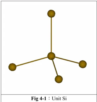
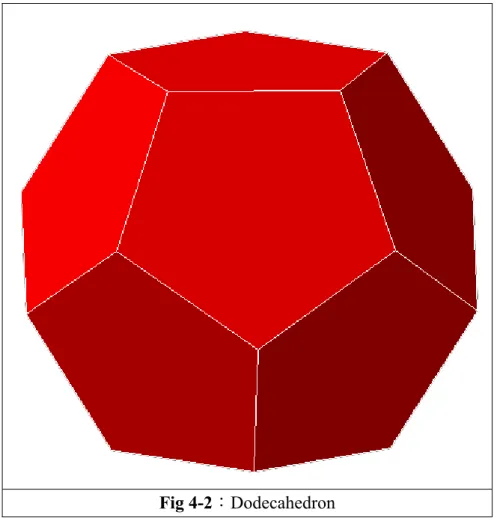
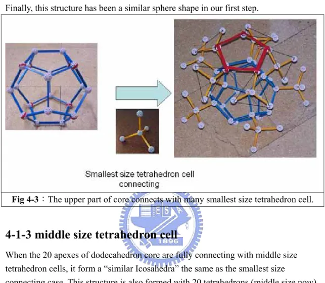
4-1 The concept of constructing Diamond structure QD model.54

4-1-1 Dodecahedron core...55

4-1-2 smallest size tetrahedron cell...55

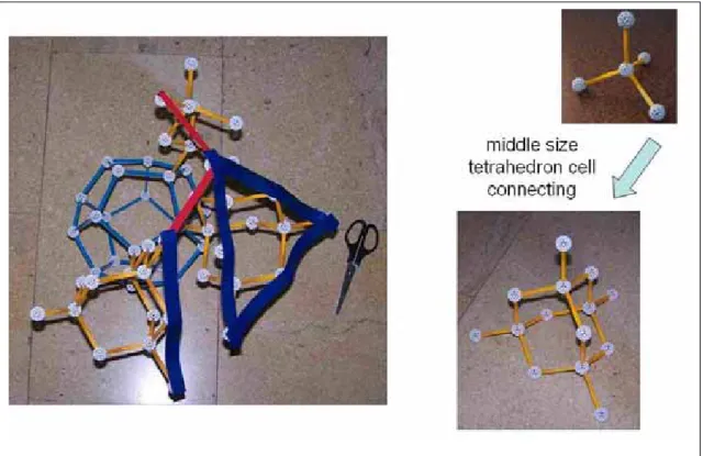
4-1-3 middle size tetrahedron cell...56

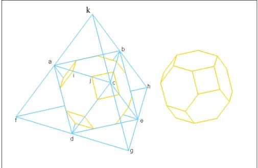
4-1-4 giant size tetrahedron cell...57

4-2 Model a bulk like QD from small to big ...59

4-3 The introduction of first-principle calculation...62

4-3-1 Hatree and Hatree-Focd Equations...62

4-3-2 Density Functional Theory ...65

4-3-3 Kohn-Shan theory and Local Density Approximation

(LDA) ...67

4-4 Relation between Eg and photon lifetime ...68

Chapter5：Conclusion

...71

Appendix A：The preparation of non-colloid sample ...73

Appendix B：Alignment of Raman Scattering System ...73

Appendix C：The optical element of time resolved system...74

Main Optical Unit ...74

Sample Holder...75

Detector ...75

TCSPCD Data Acquisition...75

Appendix D：Construction of the QD model with Zinc-Blend

structure...76

Part I：EXPERIMENT

Chapter1：Introduction

1-1 Introduction of high pressure

Besides the physical parameter such as temperature and the chemical composition, pressure effect can efficiently decrease the distance between atoms.

In general, high-pressure researches can be mainly classified into two parts. One is to investigate phenomena that occur only or primarily at high pressure. The other is to gain a better understanding and characterization of matter or processes, which occur at atmosphere pressure. In our purpose, we employ high pressure technique to change the size of quantum dot and its structure to alter the energy band gap to see which might alter the photon lifetime in transmission. Pressure induced phase transition of semiconductor to metal is also important in studying on

characteristic of the semiconductor QD. In general, metallic behavior is expected for most semiconductors at high pressures since pressure-induced structural phase

transformations occur when the atoms become more closely packed. Although we can not overemphasize the importance in understanding the effects of pressure on

structural and electronic properties of semiconductors, however studies of these materials under high pressure are not only interesting but also heuristic. In particular, the pressure-induced structural phase transition from semiconductor to metal is one of the major subjects in theoretical and experimental researches for decades. In order to investigate the novel physical properties of nano-crystal at high pressure, several high-pressure techniques were developed. For instance, thick-walled cylinders, multiple piston apparatus, and high-pressure pistons etc. are all instruments for generating high pressure. Among these technologies, diamond anvil cells (DACs) are usually used.

1-2 Introduction of QDs

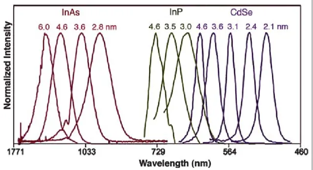
QDs, which are only a few nanometers in diameter, exhibit discrete size-dependent energy levels. As the size of the nanocrystal increases, the energy gap decreases, yielding a size-dependent rainbow of colors. Extensive tunability, from ultraviolet to infrared, can be achieved by varying the size and the composition of QDs (Fig1-1),

enabling simultaneous examination of multiple molecules and events. For example, small CdSe nanocrystals (∼2 nm) emit light with wavelength in the range between 495 to 515 nm, whereas larger CdSe nanocrystals (∼5nm) emit between 605 and 630 nm.

QDs have several dramatically different properties compared to organic fluorophores, one of which is their unique optical spectra. As illustrated in Fig1-2, organic dyes typically have narrow absorption spectrum, which means that they can only be excited within a narrow window of wavelengths. Furthermore, they have asymmetric

emission spectra broadened by a red-tail. In contrast, QDs have broad absorption spectra, enabling excitation by a wide range of wavelengths, and their emission spectra are symmetric and narrow. Consequently, multicolor nanocrystals of different sizes can be excited by a single wavelength shorter than their emission wavelengths, with minimum signal overlap.

Figure 1-1：Emission spectra of several semiconductor nanocrystals showing their

size- and composition-dependent emission character. Red, green, and blue series represent different-sized InAs, InP, and CdSe nanocrystals, respectively. The sizes of the nanocrystals are indicated above their corresponding spectra.

Figure 1-2：Excitation (dotted line) and fluorescence (solid line) spectra of

fluorescein (top) and a typical water-soluble QD (bottom). The excitation wavelength was 476 nm and 355 nm for fluorescein and QD, respectively.

Figure1-3：Comparison of fluorescence intensities between QD 608 (emission at

608 nm) and Alexa 488 after continuous illumination.

QDs are stable light emitters owing to their inorganic composition, making them less susceptible to photobleaching than organic dye molecules.

This feature has been demonstrated in a number of biological labeling experiments where the photostability of QDs was compared with commonly used fluorophores, such as rhodamine, fluorescein, and Alexa-Fluor (Fig1-3). This extreme photostability makes QDs very attractive as the probes for imaging thick cells and tissues over long time periods—a challenging task that necessitates collection of multiple optical sections without damaging the specimen. In addition, the two-photon cross-section of QDs is significantly higher than that of organic fluorophores, making them quite well suited for examination of thick specimens and in vivo imaging using multiphoton excitation.

Another interesting characteristic of QDs is their fluorescence lifetime of 10 to 40 ns, which is significantly longer than typical organic dyes or auto-fluorescent flavin proteins that decay on the order of a few nanoseconds.

Combined with pulsed laser and time-gated detection, the use of QD labels can produce images with greatly reduced levels of background noise.

There are also some photophysical properties of QDs that can, in some cases, be disadvantageous. One of these is the property referred to as blinking, that is, QDs randomly alternate between an emitting state and a non-emitting state. This intermittence in emission of QDs is universally observed from single dot, which imposes some limitations in QD applications requiring single-molecule detection.

However, there is limited evidence suggesting that QD blinking can be suppressed on some timescale by passivating the QD surface with thiol moieties, or when using QDs in free suspension. It has also been reported that QD fluorescence intensity increases upon excitation, an event referred to as photobrightening. Although in most cases this property can be advantageous, it is problematic in fluorescence quantization studies. Both blinking and photobrightening are linked to mobile charges on the surfaces of the dots, and although the prospects are good that they can be eliminated, for the time being these should be considered as limitations of QDs.

1-3 How to produce CdSe/ZnS QD

The investigated colloidal core/shell CdSe/ZnS QDs were synthesized by the following procedure. 0.30 g of cadmium oxide (CdO), 1.30 g of

tretradecylphosphonic acid (TDPA) and 25.0 g of tri-n-octylphosphine oxide (TOPO) were loaded into a 250 mL flask and heated to 320。

C under argon flow. After the CdO was totally dissolved in TDPA and TOPO, the solution was cooled to 300。

Cand 4.45 mL of selenium stock solution (0.5 M of selenium solution in tributylphosphine, TOP) was injected. 1.5 mL of precursor solution (made by mixing a 1.75 mL of ZnMe2 (2.0 M in toluene) and S (Si(CH3))2 in TBP) was then added drop-wise into the mixture to cover a layer of ZnS. A 20 mg of TOP/TOPO capped CdSe/ZnS QDs was mixed with a 200 mg 11-mercaptoundecanoic acid (MUA) in a reaction vessel to synthesize the carboxylated QDs. Methanol was added and the pH value was adjusted to about ten with tetramethylammonium hydroxide. The mixture was heated under reflux for 2 hours. After it was cooled to room temperature, the resulting water-soluble QDs were precipitated with tetrahydrofuran and separated by centrifugation.

1-4 Research motivation

High pressure technology is one of the important techniques in the study of lattice structures. Our purpose is to study the structure change of QD induced by high pressure. The optical spectrum, ex Raman, PL, and time resolved spectrum were used to study the structure change induced by pressure.

Raman vibration mode presents some knowledge about the lattice composition, the vibration type of atoms and the ionicity or covalency of lattice. The pressure

dependence of energy band edge in QDs can be gotten by measuring PL spectrum in high pressure. However, we know the shift of emittion wavelength under high

pressure is not only depend on the lattice structure change of QDs induced by the pressure, but also on the contribution of electron-phonon interaction. These all need to be realized by measuring the Raman and PL simultaneously.

Secondly it is interested to realize the mechanism of radiative decay rate in QDs i.e. base on the quantum optics to predict pressure dependence of radiative decay rate of QDs. By the measurement of time resolve spectrum, it is hopeful to verify the theoretical result by our experiment.

Finally we wish to study the band edge shift induced by the structure change of QD at high pressure by first-principle calculation, and hope to find out some possible

conclusion in our study.

Chapter2： Experiment apparatus

In this chapter, we will introduce the experimental set-up and the technique that were used in our experiment. These techniques include：the high pressure technique, Raman Scattering spectrum measurement, photo luminance measurement and time-resolved spectrum measurement

2-1 High pressure technique

2-1-1 Principle of applying pressure

The instruments and methods that have been employed for the generation of high pressure are probably more diverse than those in any other field of instrumentation. Pressure-generation method can be divided into three categories corresponding to existing domains of high-pressure method. The first category deals with hydraulic technique for the compression of fluids. This concerns, as a rule, pressures up to 1.4GPa, or at most 1.8GPa, which are applied to large volumes of fluid（1mm3）. The second category deals with the compression of large-volume solid samples in the range from 2 to 20-30GPa. This is the domain of high-temperature high-pressure experiments in material science and geophysical studies. In these studies, quite different instrument and methods must be used. The third category deals with diamond anvil cell（DACs）. Although, in principle, these cells are not difficult, in practice they have such original characteristics and widespread applications that is almost the most popular instrument used in high-pressure experiments.

has grown rapidly since the development of the diamond anvil cell. The principle of the technique is as follows. A sample incorporated with fluid, which acts as a

pressure-transmitting medium, is placed inside a small aperture drilled through a thin sheet of metal called gasket. Pressure is applied to the sample plus fluid system by mechanically forcing the two diamond faces closer together. Depending on the gasket material, aperture size, and the diameter of diamond face, pressures in the order of one mega-bar can now be achieved in the laboratory.

2-1-2 Diamond Anvil Cell

We use diamond-anvil cell (DAC) to generate high pressure in our experiment. It is currently the most popular instrument for the study of materials under high pressure. It has revolutionized high-pressure research, not only because it can easily reach a pressure near that in the center of the earth, but also because it admits varied

measurement techniques for the study of matters under such conditions. Fig2-1 shows the basic set-up of DAC. It is the outer part of the whole DAC. The diamond mounts are sticking on the hemispherical mount (Fig2-2). These are called the “rockers”. They can be translated for centering and is locked in position by adjusting the x and y axes, and the rocker can be tilted in its socket to secure parallel alignment of the anvil flats, as determined by the optical interference fringe pattern. In Fig2-3, a metal gasket with a drilled hole is placed between the two opposed diamond anvils. The hole was drilled on the gasket as sample chamber. In this chamber, the sample, pressure media, and ruby powder were placed.

This chamber is subjected to pressure when a force squeezes the two opposed diamond anvils together. Samples are compressed by the turn of DAC’s screw,

making the two opposed diamonds pressing mutually. A huge pressure is then created. The cell can routinely be used to ~ 60kbar pressure, depending on the diamond size. In most DAC, the diamond is usually in the 0.2~0.4 carrot range (1 carrot = 1/15 gram), and within this range the smaller the face is usually better. Diamonds for the anvil are usually selected from brilliant-cut gem stones. The selection of the diamonds and size depend upon the type of DAC and the nature of the investigation.

Fig2-1：The basic set-up of DAC

Fig2-3 The illustration of applying pressure

2-1-3 Gasketting, and Pressure Medium

The early work performed in the DAC was done on solids that were pressed between the diamond anvils without the use of a gasket. These conditions provided a highly non-hydrostatic environment for the solid.

Studies demonstrated that a pressure gradient existed under these conditions that were parabolic in nature, with pressures in the center reaching l.5 times those on the edges. Thus, any pressure measured under these conditions was basically an average pressure. Van Valkenburg (1963) first used a gasket with the DAC. The use of a gasket inserted between the diamond anvils and the immersion of crystals in a fluid were major advances in the use of the DAC. Fig2.4 shows the sectional view of the gasket indentation and the sample chamber. The metal gasket not only extends the life of a pair of anvil, but also allowed the sample to be compressed in a fluid

pressure-transmitting medium, so they can provide a truly hydrostatic environment for the sample. In a non-hydrostatic situation, the pressure of unknown value often

gasket for the containment of the pressure medium is a very important point for hydrostatic pressure creation in DAC. Some debate exists as to whether simply using a gasket between the diamond anvils without fluid provides sufficiently hydrostatic conditions to allow the worker a degree of confidence that the calibration of pressure in this situation is not an average pressure. It is probably true that the use of a gasket will reduce the pressure gradient more than those obtained when no gasket is used, but the uncertainty as to the quantity of the applied load absorbed by the gasket presents a problem.

Fig2.4：The sectional view of the gasket indentation and the sample chamber

In order to generate a hydrostatic pressure environment for sample, a fluid pressure medium is required. In this technique, placed the solid of interest under virtually hydrostatic conditions, and pressure calibrations became more meaningful, especially when one could observe changes under a microscope. Various fluids have been used, but a 4:1methanol-ethanol mixture has proved to be very popular. Unfortunately, the use of fluids is valid only to ~ 100kbar, since most liquids become solids above this pressure. De-ionized water (DI water) is also considered to be a pressure medium, but it transfers to solid ice VI and ice VII at 0.6 and 2.1GPa, respectively. However, previous study showed that the R1-R2 splitting in ruby fluorescence was maintained well up to 16.7GPa; therefore, it seems not to be a serious problem before reaching to this pressure.

In the work of Lin et al, [ref7] such a splitting was well recorded up to 36GPa. Hence, DI water seems to be a suitable pressure medium in high-pressure studies. For this reason we choose DI water as the pressure-transmitting medium in our experiment.

2-1-4 Pressure Calibration

Various methods of pressure calibration involving the DAC have been used. In early year’s pressure in the DAC was estimated by calculating force over area, the known fixed point, and internal markers such as NaCl or silver in high-pressure X-ray studies. These methods are not convenient and are often proved to be inaccurate.

In 1972 a major development occurred in the calibration of pressure in the DAC. This breakthrough was successful because of the use of visual microscopic studies in the DAC. Foreman et al. first calibrated the shift of the R-line ruby fluorescence peaks as a function of pressure in the DAC, and demonstrated that this shift could be used as a convenient internal pressure-calibrate. The technique incorporates a ruby crystal with the sample of interest and measures the pressure dependence of the sharp ruby R1 line fluorescence. Actually, two kinds of fluorescence with different wavelength are excited (R1 and R2 at 692.8 and 694.2 nm), and both dependencies can be followed simultaneously. The fluorescence’s are induced by an Ar+ or a Cd-He laser.

Ruby consists of Al2O3 doped with Cr2O3, in which some of the Al3+ ions replaced by Cr3+. Normally, Cr3+ in a cubic field would show a single band due to the spin

transition 2E→4A2 . In ruby the Cr3+ occupies an Al3+ site, but being of different size, such that it assumes a lower symmetry. This splits the states of the Cr3+ ion, forming an A-symmetric quartet ground state and a doubly degenerate first-excited state with E symmetry, as shown in Fig2-5. The combined effects of the trigonal field and spin-orbit coupling further splits the first excited state into E3/2 and E1/2 states

separated by 3.6meV. The electronic transition E1/2 → A and E3/2 → A give rise to the R1 line at 6942A and R2 line at 6928A, respectively. Those so called R-lines are the active transitions in the ruby laser. Under high pressure these shifts to higher wavelengths and the shift is measured linearly with increasing pressure. The accepted value for the ruby R-line shift is 0.365Akbar-1. In addition to this linear dependence of fluorescence on pressures, the line shape of the ruby fluorescence spectrum can also be used as a measure of the degree of hydrostaticity in the DAC sample chamber. Due to its high intensity and sharp line width (7.5 Å), only a small ruby chip is necessary for pressure calibration. Also, because of the acceptable pressure

dependency (0.36 Å kbar-1) and linearity at lower pressures ruby scale is really a rapid and dependable method. Despite of these advantages, ruby calibration still has its limitation. First of all, ruby has a significant temperature coefficient (0.068 Å ℃-1) in the same direction (red) for both temperature and pressure. Its thermal line broadens with pressure, causing R1 and R2 to overlap and limiting its use for pressure

calibration to 300℃. Less heating of the ruby will cause expansion along the axis, which results in lower symmetry, and spin-orbit coupling will increase R2 ΔR~ 29.3

cm-1 at 150 K to 29.7 cm-1 at 293 K.

Since both temperature and pressure cause a decrease in R1 and R2 frequencies, it is possible to overestimate the pressure if local heating occurs (e.g., heating in a laser). Second, there are some uncertainty in linearity of extrapolated dependency at mega bar pressure and pressure broadening of both R1 and R2 at pressures > 1Mbar. Also, the requirement of laser excitation for fluorescence may be prohibitive in small laboratories or schools (the fluorescence of ruby is very weak at low pressure; a highly sensitive spectrophotometer is needed to measure this fluorescence). Finally, values of ΔR will change under non-hydrostatic pressures.

Fig2-5：Energy level of Cr3+in Al₂O₃. The transitions of E_1/2→A and E_3/2→A give

rise to R1 and R2 lines, respectively.

2-1-5 The high pressure experiment process

A. Sample Preparation

Our samples are the colloidal quantum dots which are already in the di-water: the most common pressure media. We can load our sample in drilled gasket directly. On the contrary, samples are not colloidal ex: Al1-xInxP which is bulk sample that we need to deal with carefully. (See appendix A)

The procedures for adjusting the diamond anvil cell include the correctly setting of axial and tilt alignment of DAC without a gasket. The main purpose of this procedure is to make the two diamond anvils contacted each other and paralleled mutually in order to support huge force uniformly over the whole diamond flat. Before alignment, we must first clean the faces of diamonds thoroughly with Q-tips moistened by acetone. This cleaning action must be done under a microscope in order to check if the faces are completely clean. The faces should be free of any dirt otherwise it will cause misalignment. After cleaning, it is ready to begin the cell alignment in two parts.

1. Axial alignment: Bring carefully the two diamond anvils in direct contact and make sure that they are coaxially centered. If the two flats are not in suitable positions, use the two“adjusting screws＂set in mutually perpendicular directions to adjust the rocker of cell until the faces of diamond become flat and parallel.

2. Newton ring alignment: By applying the theorem of Newton ring, we are able to check further the parallelism between two diamond faces.

If the two anvil faces are not parallel, we will observe some optical interference fringes, which are formed from white light transmitted through the contact diamonds, under a microscope.

C. Gasket preparation

In our work, we use stainless steel T304, which can maintain pressure up to about 35GPa, as the material of gasket. The procedure for gasket preparation can mainly be divided into two parts. First we have to pre-press the stainless steel gasket to about 15GPa. Before this step, it is necessary to clean the gasket thoroughly. And also, the distance between gasket and diamond flat must keep at about 200μm in order to provide enough space for gasket pre-pressing. The whole procedure is listed below: 1. Choose suitable rings to make the distance between gasket and

diamond below the gasket being around 200μm and seat the gasket on the diamond below.

2. Bring the two diamond cells in direct contact and compress the cell to make a slight indentation on the gasket.

3. Separate the two diamond cells, and put a few ruby chips in the indentation made previously. Here ruby is used for pressure calibration.

4. Bring the two cells in contact again, and then put it in the body for generating high pressure. Turn the screw head clockwise slowly until the pressure necessary is

reached and then loose the screw. Taking the gasket out of the cell, we can see a deeper indentation under a microscope.

150μm, which is much smaller than the initial value (around 300μm). Now we have to drill a hole at the center of the indentation of the gasket. This hole is drilled by the micro electric discharge drilling system. Usually the gasket hole is 90μm in diameter. In order to make a whole circular hole, it is necessary to make sure that the drilling needle is straight and perpendicular to the indentation surface.

For this purpose, it is helpful to flatten the gasket blank.

D. Sample loading

The hole on the gasket is prepared as a chamber for sample loading.

Since the size of this chamber is very small, our samples must be thinned and cleaved into a size smaller than the pressure chamber. This way, the chamber can thoroughly surround the sample without destroying the sample. Sample loading is therefore quite difficult and must be carried out under a microscope. The procedure of sample

loading is described as follows:

1. Choose suitable rings to make the indentation of the gasket directly contact with the flat of the diamond and seat the gasket on the diamond anvil below.

2. Uniformly place a few ruby chips (about 1μm) on the upper diamond flat for pressure calibration.

3. Using needle inhale a little sample（colloidal quantum dot in di-water）to inject into sample chamber, by the way, di-water is pressure transmitting medium.

Then bring the two cells in contact as soon as possible（this is to prevent sample from coagulating）and turn the screw to tighten it a little. Now we can start various optical measurements.

2-2 Raman scattering experiment

Figure2-6 is our Micro Raman Scattering experiment setup in NHCTC. The system is

composed of a Kr ion laser, main microscope, CCD detector, spectrometer, and data analysis computer shown as figure. You can see the laser reflected by two mirrors is going into the main microscope and is focus by objective then meet the sample to produce Raman scattering process. In this chapter, we will introduce how these components work.

Fig2-6：The configuration of Micro Raman Scattering experiment in NHCTC.

At first we simply introduce the process of Raman spectrum measuring experiment. The rough figure of the internal part of main microscope is shown in Fig2-7.

See from Fig2-7, the laser（green line）is coming from input and is reflected by mirror M1, after pasting two attenuation lenses then arrive mirror M2. After two reflection by a pair of reflection mirrors, laser light achieves notch filter which like a

beamspliter can reflect incoming laser (i.e.: the green line) and filter unwanted laser in scatted light（i.e.: the pink line）. Notch filter plays an important role to avoid the intensity of backing laser exceeding the scatted light which is relatively weak than laser. The laser reflected by notch filter（green line）goes into the objective and is focus to hit sample to produce Raman scattering process. The scatted light（pink line） also collected by objective then comes back to notch filter again. It is important that noise laser is filtered by notch filter; only the scattering light can pass. The passed light is reflected by M3 and M4 mirrors and goes into the confocal hole which is set to make sure the single is coming from the focal point of incident laser. By passing through confocal hole, single is reflected by mirror M5, then finally go into the fiber and enter into spectrometer. The spectrometer divides light into many different wavelength regions and CCD detector count intensity of different wavelength light. By properly choosing integrating time and average times, computer shows the Raman scattering spectrum to us. The alignment of the optical units in our Raman experiment is described in Appendix B.

Fig2-7：The internal part of main microscope of the Micro Raman Scattering apparatus.

2-3 PL and photon lifetime spectrum experiment

2-3-1 Instrument Introduction：

In order to exploit the merits of a powerful analysis tool such as time-correlated fluorescence spectroscopy, one must in some way or other record the time dependent intensity profile of the emitted light. While in principle, one could attempt to record the time decay profile of the signal from a single excitation-emission cycle; there are practical problems to prevent such a simple solution in most cases. First of all the decay to be recorded is very fast. Typical fluorescence from organic fluorophores lasts only some hundred picoseconds to some hundred nanoseconds. In order to recover fluorescence lifetimes as short as e.g. 500ps, one must be able to resolve the recorded signal at least to such an extent, that the exponential decay is represented by some tens of samples. This means the transient recorder required would have to

sample at e.g. 50ps time steps. Clearly this is hard to achieve with ordinary electronic transient recorders. Secondly the light available may be simply too weak to sample an analog time decay. Indeed the signal may consist of just a few photons per

excitation/emission. Then the discrete nature of the signal itself prohibits analog sampling. Even if one has some reserve to increase the excitation power to obtain more fluorescence light, there will be limits, e.g. due to collection optic losses, spectral limits of detector sensitivity or photo-bleaching at higher excitation power.

The solution is Time-Correlated Single Photon Counting (TCSPC). Since with periodic excitation (e.g. from a laser) it is possible to extend the data collection over multiple cycles, one can reconstruct the single cycle decay profile from single photon events collected over many cycles.

The method is based on the repetitive precisely timed registration of single photons of e.g. a fluorescence signal. The reference for the timing is the corresponding

excitation pulse. As a single photon sensitive detector, one can use a Single Photon Avalanche Photodiode (SPAD). Provided that the probability of registering more

than one photon per cycle is low, the histogram of photon arrivals per time bin represents the time decay one would have obtained from a single shot time-resolved analog recording. The precondition of single photon probability can (and must!) be met by simply attenuating the light level at the sample if necessary. If the single photon probability condition is met, there will actually be no photons at all in many cycles. Figure2-8 and Figure2-9 illustrate how the histogram is formed over multiple cycles：

Fig2-8：The illustrate of how SPAD detect photon in many cycles to form TCSPC

Fig2-9： The histogram is formed by recording photons after many process in Fig 2-8

The histogram is collected in a block of memory, where one memory cell holds the photon counts for one corresponding time bin. These time bins are often referred to as time channels.

In practice the registration of one photon involves the following steps: first the time difference between the photon event and the corresponding excitation pulse must be measured. For this purpose both signals are converted to electric signals. For the

fluorescence photon this is done via the single photon detector mentioned before. For the excitation pulse it may be done via another detector if there is no electrical

sync signal supplied by the laser. Obviously all conversion to electrical pulses must preserve the precise timing of the signals as accurately as possible. The actual time difference measurement is done by means of fast electronics which provide a digital timing result. This digital timing result is then used to address the histogram memory so that each possible timing value corresponds to one memory cell or histogram channel. Finally the addressed histogram cell is incremented. All steps are carried out by fast electronics so that the processing time required for each photon event is as short as possible.

When sufficient counts have been collected the histogram memory can be read out. The histogram data can then be used for display and e.g. fluorescence lifetime calculation.

2-3-2 Configuration and Standard Components：

which is a powerful, newly-developed instrument capable of Fluorescence Lifetime Imaging with Single Molecule Detection sensitivity. It contains the complete optics and electronics needed for recording virtually all aspects of the fluorescence dynamics of microscopic samples or femto-liter volumes. The instrument gains its exceptional sensitivity and flexibility in combination with an unprecedented ease of use from a unique fusion of miniaturised and highly sophisticated state-of-the-art technologies. For the first time, these technologies enable to run an instrument of comparable complexity and power to be operated in routine work, without having to spend more time on instrument maintenance than on original scientific content. The underlying key technologies are the proven Pico-second Diode Lasers and the Time-Correlated Single Photon Counting electronics developed by PicoQuant, complemented by state-of-the-art piezo-scanning technology and optics from industry leaders.

The insight of “Micro-Time 200 fluorescence lifetime microscope system” is shown in Fig2-10.

Fig2-10：The insight of Micro-Time 200 fluorescence lifetime microscope system.（blue line

is the incoming laser and pink line is the signal of laser excitation.）

2-3-3 Overview：

excitation which come from fiber1 entering into the main optical unit is collected by a convex lens with that become a parallel light（blue color）. After reflecting by a mirror, this parallel light comes to beam-splitter b which splitter light into two components; one goes to photodiode while the other directly pass the beam-splitter. Photodiode is an apparatus that told you the intensity of incoming excitation. The passing light is then reflected by beam-splitter a and enters the microscope (Olympus IX 71) to excite the sample; then signal (fluorescence of sample；pink color) is collected by objective and come back via the original path and pass beam-splitter a again. The signal is then traverse through lens1, confocal pinhole and lens 2. Confocal pinhole is making sure the signal is excited from focal point of laser. In order to measure PL and lifetime at the same system, we use beam-splitter c to divide light into optional

excite port 2 which is connected to a spectrometer (Trix320) while the other light

pass through beam-splitter c. The passing light reflected by two mirrors（Mirror a,b） enters dector1 to record life time. Near dector1 there are filter2 to decrease light intensity and shutter2 to control light passing or not. Under this setup, we can use the lock gate to control signal into spectrometer or detector1, the former is used to measure PL while the later is for recording lifetime.

We will introduce in detail the use of the entire component in Appendix C.

Chapter3：Experiment result and discussion

3-1 Result

3-1-1 Raman spectrum

Our sample in this experiment is the 630nm emission colloidal core/shell CdSe/ZnS QDs with core diameter equal to 10 nm and thickness of shell equal to 1 nm. In this experiment we can find that both the vibration mode of CdSe and ZnS appears in our Raman spectrum. Our data shown in Fig3-2、3 agree with the Raman spectrum obtained by Ref1[See Fig3-1]. The peaks presented in Fig3-2、3 are the CdSe LO mode at ~210cm-1, CdSe 2LO mode at ~420 cm-1 and ZnS LO mode at~300 cm-1. By the way, the data shown in Fig3-2, 3 are coming from the same QDs observed at different days for double check.

As we had just mentioned that the experimental data shown below are observed at different days, the data shown in Fig3-2 is observed on Oct-24/2005. In this

observation presented before the occurrence of phase transition. The other experiment data shown in Fig3-3 is obtained Nov-08/2005 and this data is decomposed into three parts, one is for the process of adding pressure until the peaks of CdSe LO and 2LO disappears (phase transition) [Fig3-3], the other is to add pressure up to the highest one(36.72GPA)after phase transition[Fig3-4], and the final one is for the decreasing pressure from the highest pressure down to 3.44GPA which is shown in Fig3-5. The data shown in Fig3-6 is the whole Raman spectrum in this experiment；include the loading pressure and unloading pressure process.

From our experiment data shown in Fig3-2 and Fig3-3 , one can easily see that：in the loading process the LO mode, 2LO mode of CdSe and the LO mode of ZnS are all shift to high frequency at first.（blue shift）

When the pressure approaches nearly 7GPA, we find that both LO peak and 2LO peak of CdSe start to disappear and the ZnS LO mode remains exist up to 35GPA as shown in Fig3-2 and Fig3-3. From this information we deduce that the core CdSe begins phase transition at about 7GPA, compared to the pressure-induced phase transition in bulk CdSe at about 3 GPA. We label this phase transition in QDs as the “Phase Transition I”. Due to the core-shell structure of QDs, we can reasonably assume that this retarded pressure-induced phase transition in core comes from the screening effect of ZnS shell.

By synchronal measuring the PL spectrum and Raman spectrum, we can find some interesting information by comparing these two data. The most important

phenomenon is that：the PL spectrum can’t be explored after phase transition had been found in QDs from Raman spectrum. This gives us information that the core in QD may become metal phase for two reasons：

1. When QD is under phase transition, the LO peak and 2LO peak of CdSe start to disappear in Raman spectrum; this implies PHI to occur in core of QDs.

2. QD is not under fluorescence after PHI; this verifies that the metal phase of core happens in QD.

From the band diagram of bulk CdSe with rocksalt structure as shown in Fig3-7, one can see that the conduction band overlaps the valance band; this verifies the

occurrence of the metal phase of CdSe.（the band diagram is calculated by ab-initio） We believe the structure difference caused by phase transition in QDs is just the same as it in bulk CdSe whose structure is from zinc-blende to rocksalt. In other words we believe after phase transition the structure of core in QDs is the rocksalt structure the same as the bulk behavior.

After phase transition І, the LO and 2LO mode of CdSe disappears and a new

undetermined peak appears nearly ~156 cm-1, this new peak is very interesting due to the fix position of this peak as pressure varies! After increasing the pressure so that it

is larger than ~7GPA, the peak is always presented and the position of it unchanged until pressure goes up to 34GPA. Even if the pressure reduced below 7GPA that come to the same situation. (See the data shown in Fig3-5, this peak is also present even the pressure is reduce to be lower)

The LO signal of ZnS is very weak in 1108 data, it is almost unrecognizable before phase transition І, but after phase transition І it can be recognized even if it is still weak and nearly disappears at 36.72GPA（See Fig3-4）. At first, this pressure might be regarded as another phase transition, however by comparing with the 1024 data

（Fig3-2）, we see the signal of ZnS is always distinguishable up to pressure equal to

34.11GPA. For this reason it should not be another phase transition and may come from the defect of sample.

While in the unloading process, the LO mode of ZnS starts to be red shift along the original path of loading process.（see Fig3-5） When the pressure reaches 3.44GPA, the LO mode of CdSe appears again and its peak position corresponds to the data of loading process, however, the CdSe 2LO mode does not appear again. This

phenomenon makes us to believe that CdSe might not reduce back to the zinc-blende structure again. Thus the phase transition І is an irreversible one.

Fig3-1：Raman spectrum of CdSe/ZnS QD’s with a shell thickness 3.4 ML excited by a 476.5-nm line of

an Ar12 laser.

Fig3-2：Raman spectrum of CdSe/ZnS QDs in di-water under different pressure.（gotten in 1024）

Fig3-3： Raman spectrum of CdSe/ZnS QDs in di-water. The pressure is added up to phase

Fig3-4：Raman spectrum of CdSe/ZnS QDs in di-water.（gotten in 1108） Pressure is added above phase transition up to 36.72GPA.

Fig3-5：Raman spectrum of CdSe/ZnS QDs in di-water.（gotten in 1108） Reduce pressure from 36.72GPA to 3.44GPA.

Fig3-6：Whole Raman spectrum of CdSe/ZnS QDs in di-water.（gotten in 1108）

3-1-2 Photon luminescence

In this chapter we only focus on how energy band gap of QDs changed under the applying of pressures. In this experiment, our sample is a quantum dot with radius in 5nm with ZnS shell cladding which thickness is 1nm.

The first thing we need to remark is that only PL spectrum below the pressure of phase transition is obtained. This is because as Raman spectrum exhibits the occurrence of phase transition, the PL spectrum is no longer to be measured.

From our experiment data shown in Fig3-8 we see the band gap Eg of QDs has obvious pressure dependence. To explain the reason we follow the discussion in ref. [2] ；in this paper the QD has two size regions for investigating the pressure

dependence.（Rigion1: QD’s radius＜a0；Rigion2：QD’s radius≧a0, where a0 is the effective Born radius which is 5.6nm for CdSe） By the way, the QD in ref. [2] is the pure CdSe QD without shell.

They believe that the mechanism of the shift of band edge under pressure is due to the electron-phonon interaction of polaron. For small size QD, the previous experiment data shows zero pressure parameter(dE/dP=0) and they interpret that is because the strong coupling of defect levels in QD to the core levels due to the strong confinement of the exciton wave function. This results in an effect that the excitonic levels being primarily perturbed by the particle size instead of electron-phonon (el-ph) interactions. This is because that the el-ph interaction is not dominant in this small size regime and the pressure dependence doesn’t occur in low pressure. However for the larger QD size（r=40A）, the bulk like pressure dependence is observed as expected. In this thesis, all the pressure parameters are all obtained for lower pressure (up to 0.25GPA), and no lattice structure change are concerned. They only focus on the variation of the polaron energy with the lattice ionicity for different sizes of QD.

Ref. [2] mainly studied the pressure parameter（dE/dP）of different size QDs. The diagram of dE/dP parameter versus QD’ size is shown in Fig3-9. The pressure parameter of QDs with a radius of 22.5A is about 80meVGPa-1 while that of the QD with radius of 40A is about 40meVGPa-1which is close to the bulk values of 37.5 meVGPa-1. From the experiment data of the 5nm (in radius) core/shell CdSe/ZnS QD, the band edge-pressure curve can be fitted by a polynomial, obtain as：

as shown in Fig3-10.

On contrary, the bulk CdSe Eg-pressure curve can be fitted by: Egbulk=1.71+0.0375P eV, as shown Fig.3-11.

Thus, the pressure parameter (dE/dP) of our QDs is almost equal to the bulk’s value at low pressure（for low pressure the term of P2 can be ignored in (3.1)）, and this agree with the prediction of ref. [2].

Our result shows that when QDs are in high pressure, the pressure dependence of band edge is reduced, and this is the reason that the negative term is contained in equation (3.1). What cause this phenomenon? This means the lattice become more and more covalent with adding pressure.（lattice become more and more covalency thus the electron-phonon interaction become weak；reduce the pressure dependence of Eg） We will discuss this effect with quantification in chapter3-2-2.

Fig3-8：The 5nm radius CdSe/ZnS QDs fluorescence patterns vs pressure. （gotten in 1108）The number above

peaks are the correspond energy of fluorescence.

Fig3-9：The pressure parameter of different size CdSe QDs.ref2

The pressure parameter of bulk CdSe is 37.5(meV GPA-1)

Fig3-10：Pressure dependence of band edge（get from PL peak）in 5nm radius CdSe/ZnS QDs. The dot is the experiment

data.

The red solid line is the fitting line of experiment data.

Fig3-11：Pressure dependence of band edge in bulk CdSe at 295K.ref5

Phase transition happened at nearly 2.9GPA.

3-1-3 Photon life time result

In this section, we will focus on the experiment data of PL spectrum and photon life time spectrum to investigate the relation between band edge and the radiative life time of QDs. In this experiment, we also study the pressure effect on the photon life time of QD. In our experiment, two different sizes QDs; i.e. 3.5nm radius（emits yellow colorλ= 530 nm） and 5nm radius（emits red colorλ=630 nm）CdSe quantum dots and

with 1nm thickness ZnS shell cladding are used.

Fig3-12a, b show the PL spectrum and life time spectrum under different pressures of

3.5nm radius QD. One can note that the Eg increases as the pressure is increased; the photon life time becomes faster as the Eg of QD is increased. (Fig3-12b)

For 5nm radius QD, the corresponding result of Eg and life time are presented in

Fig3-13a、b.

We use a Gaussian curve to fit the PL peak and the fitted data is listed as shown in

scale as shown in Fig (b). The curves are then fitted, and the decay ratesτare obtained.

Change to logarithmic coordinate

Fig (a) Fig (b)

Fig3-12b and Fig3-13b show the obtained results for 3.5 and 5nm radius QDs. In Fig3-12b, one can find that life timeτ1 is slower and life timeτ2 is faster. For the 5nm radius QD, its photon life time spectrum is almost dominated by one time scale decay rate 1/τ3 as shown in Fig3-13b.

By following the previous published papers [ref.7], it is believed the one of the decay rate comes from the core state and another comes from the surface state. Thus for the large surface/volume atoms number ratio of our 3.5nm radius QD, two kinds of life times are needed. But for 5nm radius QD, thus only one decay rate is needed. (its volume/surface atoms number ratio is larger)

Fig3-12a：The 3.5nm radius CdSe/ZnS QDs fluorescence patterns vs. pressure.

（gotten in 1103）

The number above peaks are the correspond energy of fluorescence.

Fig3-12b：Left：The life time spectrum under different pressure of the 3.5nm radius CdSe/ZnS QDs.（gotten in 1103）

Right：Table of band edge, life time1 and life time 2 which are fitted from experiment data.

Fig3-13a：This figure identical to Fig3-8.

Fig3-13b：Left：The life time spectrum under different pressure of the 5nm radius CdSe/ZnS QDs.（gotten in 1108）

3-2 Discussion

3-2-1 Raman discussion

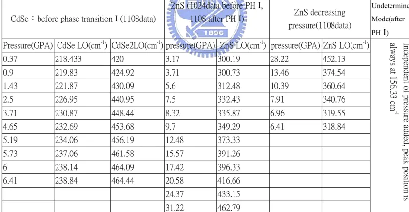
A Lorentzian form is used to fit the asymmetry spectrum as shown in Figs3-2,3,4, 5; the frequency of different phonon modes and the corresponding pressures are listed in

Table І.

The loading (black) curve is compared with the unloading curve (red) as shown in

Fig3-15; it can be found that these two curves are almost consistent with each other.

This might be resulted from the reason that the ZnS shell doesn’t perform phase transition in the loading/ unloading processes. Only the lattice constant of ZnS (zinc-blende structure) is compressed during the applying of pressure.

The relationships of mode frequencies versus pressure can be obtained by the quadratic polynomial formulae（3.2）、（3.3）and（3.4）.

CdSe _{216.766 3.932 0.077} 2_（cm P P LO = + − ω -1 ）………...…（3.2） CdSe 2_（cm 2LO =416.569+10.057P−0.398P ω -1 ）………..（3.3） ZnS _{268.71 9.17 0.0958} 2_（cm P P LO = + − ω -1 ）………..（3.4） Undetermined mode ω =156.33+0P（cm-1）

From formula（3.2）、（3.3）we can obtain the Grűneisen parameter γi from the

following definition： dp d B V i i i i ω ω ω γ 0 0 ln ln = ∂ ∂ − = ……….（3.5）

where the bulk modulus B0 is defined as the inverse of the isothermal compressibility （53 GPA for CdSe）

and 2 is our fitting formula.

0 ap bp

i

i =ω + +

ω

By substituting formula（3.2）、（3.3）into（3.5）, we find that the Grűneisen parameter

i

γ of CdSe is a function of pressure：

p p B i LO (3.93 0.077 ) 0.9608 0.0188 766 . 216 53 0 0 _{− = −} = = = ω γ . ………...（3.6） p p B i LO (10.057 0.398 ) 1.279 0.05 569 . 416 53 0 0 2 ₌ − = − = = ω γ ………..（3.7）

Grűneisen parameter can be viewed as the degree of interaction between the variations of Raman mode versus lattice constant. One can deduce the lattice is

covalent or ionic by this parameter. In generally：ifγiis small, the lattice is covalent；

ifγiis large, the lattice is ionic.

In an ionic lattice, the polaron is easy to form i.e. electrons tend to attract the cation and exclude anion and form a quasi-particle-polaron; thus indicate strong

electron-phonon interaction, and enhance the pressure dependence of polaron energy. This will be explained again in PL and Raman discussion.

From formula（3.6）、（3.7）we see the pressure tends to decrease the lattice ionization （become more covalent）due to the second negative term ofγi. Fig3-16a is the

diagram of Grűneisen parameter versus various sizes QD.ref2 One can deduce theγ_LO of our experiment at nearly 7GPA is about 0.829 which is correspond to the 2.5nm radius QD in the covalent region in this diagram. We plot the Grűneisen parameter of CdSe LO and 2LO modes versus pressure in Fig3-16b; one can see both parameters decrease while loading the pressure and the lattice transmit from ionic region into covalent region.

CdSe：before phase transition І (1108data)

ZnS (1024data before PH І, 1108 after PH І) ZnS decreasing pressure(1108data) Undetermined Mode(after PH І)

Pressure(GPA) CdSe LO(cm-1

) CdSe2LO(cm-1 ) pressure(GPA) ZnS LO(cm-1 ) pressure(GPA) ZnS LO(cm-1 ) 0.37 218.433 420 3.17 300.19 28.22 452.13 0.9 219.83 424.92 3.71 300.73 13.46 374.54 1.43 221.87 430.09 5.6 312.48 10.39 360.64 2.5 226.95 440.95 7.5 332.43 7.91 340.76 3.71 230.87 448.44 8.32 335.87 6.96 319.55 4.65 232.69 453.68 9.7 349.29 6.41 318.84 5.19 234.06 456.19 12.48 373.33 5.73 237.06 461.58 15.57 391.26 6 238.14 464.09 17.42 396.33 6.41 238.84 464.44 20.58 416.66 24.37 433.15 31.22 462.79 I n d e p e n d e n t o f p r e s s u r e a d d e d , p e a k p o s i t i o n i s a l w a y s a t 1 5 6 . 3 3 c m -1

Table І：Lists of Raman peaks at various pressure in 5nm radius CdSe/ZnS QDs. The data of ZnS are composite of 1024 and 1108 data; others are come from the same day data.

Fig3-14：Pressure dependence of CdSe LO and 2LO Raman peaks in 5nm radius CdSe/ZnS QDs. （gotten in 1108）

Fig3-15：Pressure dependence of ZnS LO Raman peaks in 5nm radius CdSe/ZnS QDs.

（gotten in 1108）

The dots are experiment data. The solid lines are guide to eyes.

Fig3-16a：The Grűneisen parameter（exp） and el-ph coupling constant（theory）versus

CdSe QD’s size.ref2

Fig3-16b：The Grűneisen parameter of CdSe LO（down）and 2LO（up）mode in our 5nm

3-2-2 Raman and PL discussion

As we had explained in chapter 3-2-1； when loading pressure the lattice tends to become more covalent. This comes from the second negative term in Grűneisen parameter i.e.γLO =0.9608−0.0188p andγ2LO =1.279−0.05p. One can see as the

pressure is lowγLO =0.9608; which is close to the bulk’s valve 1.1

ref3_{, so they have} very similar pressure dependence due to the same strength el-ph coupling. But when pressure is about 4 or 5 GPA, the negative term inγLO becomes non-ignorable

(~0.094) and the value ofγLO becomes 0.86 which is belonging to the region of

covalent lattice.ref2 The increase in lattice covalency means the polaron difficult to form, thus decrease the electron-phonon interaction. That is the reason why pressure increasing to high we see the pressure dependence of band edge becomes unapparent in QD.

Here, we here will bring up a simple model to explain roughly the data of PL versus pressure.

Imagine what would happen when a QD is under pressure? The effect is that first the lattice constant will be compressed and second is the lattice ionicity will be changed by pressure；the later will influence the polaron energy in QD. The first effect（the pressure induced electronic structure difference results in energy band edge shift）can be simulated by the pressure induced band edge shift in bulk；however the polaron energy changed by pressure is just the main topic of our model.

At first we write down the Hamiltonian of our model：

[

iKX

]

K X iK K K K K v e e a e a K i a a K d M P V H H H ⋅ ⋅ − + + _{+ −} + = ∆ + + =

∑

∫

( 2 ) 1 ) 2 ( 2 1 2 / 1 3 3 2 απ π ω =

whereHeis the electron Hamiltonian in solid with effective mass.

The second term is the phonon energy, are the creation and annihilation operator of phonon with momentum K.

K K a

a ,+

The third term is the potential induced by lattice distortion（polaron potential）,

L C ω α = 2

= is the coupling constant in △V1 that describes the el-ph coupling strength, and C is the lattice deformation energy. ωL is the longitudinal optical phonon frequency of the lattice.

By using perturbation method (for smallα ) the eigenvalue difference except the part of lattice structure is： ₎2

10 ( 26 . 1 α α + − = ∆E

Because LO C ω α = = 2 1

, whereωLO is the vibration frequency of CdSe LO mode, thus

we can deduceα from our Raman spectrum experiment and gives： （substitute formula（3.2）intoωLO） ) 077 . 0 93 . 3 766 . 216 ( 2 2 p p C − + = =

α which is a function of pressure.

Where the =

C 2

is still an unknown parameter of our system.

Thus the total eigenvalue of the system is ： (ignore the phonon energy, because it is small)

2 0 ) 10 ( 26 . 1 ) ( −α + α =E p

E , is the electron eigenenergy determined by lattice structure, and the other terms are the energy shift induced by polaron effect.

) (

0 p

E

We assumeE₀(p)is a linear function with pressure（E₀(p)= A+bp）Because the “pressure screen effect” of ZnS shell, the inner part of QD reaches 3GPA while the outer pressure is 7GPA. We thus deduce the effective pressure parameter of QD is： (come from the structure difference contribution)

GPA eV b 0.0175 / 4 . 6 3 0375 . 0 × = = ,

where the 0.0375eV/GPA is the pressure parameter comes from bulk CdSe experiment.

Thus the total eigenvalue becomes ₎2

10 ) ( ( 26 . 1 ) ( 0175 . 0 p p p A E = + −α + α

To find out the other unknown parameters, we do the differential：（assumeα is small and ignore theα square term）

(

)

(

)

(

)

(

216.766 3.93 0.077

)

0.0175 077 . 0 93 . 3 2 0175 . 0 077 . 0 93 . 3 077 . 0 93 . 3 766 . 216 2 ) 077 . 0 93 . 3 766 . 216 ( 2 0175 . 0 0175 . 0 2 2 2 2 1 2 + − + − = + − − + = ∂ − + ∂ − = ∂ ∂ − = ∂ ∂ − − p p p C p p p C p p p C p p E = = = α

From the data of PL experiment shown in Fig3-10, we know when p≒0 the slope of the experiment data is nearly 0.0354eV/GPA, substitute this valve into the formula above it gives：

57 . 214 10 342 . 8 0179 . 0 2 0179 . 0 10 342 . 8 2 0354 . 0 ) 766 . 216 ( 93 . 3 2 0175 . 0 5 5 2 0 = × = ⇒ = × ⋅ ⇒ = + = ∂ ∂ − − ≈ = = = C C C p E p

Therefore, the unknown constant =

C 2

is determined.

Thus we can obtain a formula to predict the band edge of QDs changed by pressure

eV p p p A p p A p E ) 077 . 0 93 . 3 766 . 216 ( 57 . 214 0175 . 0 ) ( 0175 . 0 ) ( ₂ − + − + = − + = α ………（3.A）

Although we still don’t know the initial energy of the system i.e. A, but we can choose a proper value of A to fit the data of the curve in Fig3-10. We plot this equation in

Fig3-17 in a pressure range 0.9~6.4GPA to compare the experiment data as shown in

Fig3-10. One can see when pressure is high; the curve tends to be smooth just as the experiment data shows. The smoothness comes from the polaron energy, and the smaller polaron energy comes from the lattice covalency. Thus, the lattice covalence effect makes the band edge-pressure curve in QDs become smooth at high pressure.

The polaron effective mass defined as )

0034 . 0 6 1 1 0008 . 0 1 ( 2 2 * * α α α + − − ≅ m

m_pol , and the plot it

versus pressure is shown in Fig3-18. Onecan easily see the higher the pressure the lighter the effective mass, which is another evidence that the lattice of QDs becomes more and more covalent while loading pressure.

Finally we compare both the Grűneisen parameter and el-ph coupling constant versus pressure, the former is deduced from the experiment and the later is deduced from the theorem, one can see both of them has the same tendency with adding pressure；i.e. the lattice becomes more and more covalent. The figure is shown in Fig3-19.

Fig3-17：The plot of formula（3.A）

This curve tend to be smooth at high pressure, one can compare this cure to experiment data shown in Fig3-12.