Finite Element Analysis of the Lateral Crushing Behavior of Segmented Composite Tubes

Finite Element Analysis of the Lateral Crushing Behavior of Segmented

Composite Tubes

Frank Ratter1, Dennis Lueddeke1, Shyh-Chour Huang2

1.

Department of Mechanical Engineering

University of Applied Sciences Ingolstadt Ingolstadt, Germany

2.

Department of Mechanical Engineering

National Kaohsiung University of Applied Sciences Kaohsiung, Taiwan, R.O.C.

Abstract

This paper aims to develop a finite element model for a lateral crushing behavior of segmented composite tubes. In the first step, the finite element modeling is established. Then, the model is modified according to the experimental results. Once the model was proven do yield the correct results, dynamic crushing was simulated. We varied the tube's geometry and the composite's material properties to make conclusions about the optimum composite tube configuration.

Keywords: Composite Tubes, Dynamic Crushing Behavior, Finite Element Method.

1. Introduction

Offering a wide field of applications in the industry, the thematic energy absorption was already discussed in several research articles over the past years. Especially race cars that are supposed to resist energetic impacts are equipped with tubes to higher the crashworthiness and save occupants lives. A lot of the scientific articles deal with the behavior of tubes under specific loading conditions. Zeng [1] simulated the crushing behavior of composite tubes faced to axial loadings using LS-DYNA in 2004. Furthermore A. Mahdi et al. [2], did the development of the experimental data concerning the “energy absorption capability of laterally loaded segmented composite tubes”. As a continuation of former mentioned work this study deals with the simulation of the crushing behavior of laterally impacted, thin-walled composite tubes.

The experimental data was achieved by exposing the component tubes to quasi-static a lateral loading realized by two flat platens at their top and bottom. The load was applied at the top one. The total compression was 95% of the diameter and equals 95 mm. The tubes were segmented into 3 parts and bonded by epoxy resin. The geometric properties of each tube were given by a diameter of 100mm and a segment length of 50mm. This leads to a total tube length of 150mm. The failure mechanism varied throughout the different test despite constant parameters and initial conditions. Due to this the absorbed energy varied. To compensate this fact the authors decided to use an average over 3 tests in their data collection.

For this already existing experimental setup and resultant experimental data, a Finite Element Method (FEM) model is to be created. The model is validated by comparing the numerical results to the experimental data. After the model is proven to produce correct results, the quasi-static crushing conditions are changed to a dynamic impacting on the tube. The energy absorbed by the tube is recorded for this dynamic crushing, while varying the parameters "tube wall thickness" and "tube segment material". The results obtained by the FEM–Modeling allows us to make predictions about the optimal tube configuration concerning geometry and material properties for ©2007 National Kaohsiung University of Applied Sciences, ISSN 1813-3851

dynamic impact crushing.

To compare different materials or forms in their ability of energy absorption, the SEA - Specific Energy Absorbed ratio expressed in equation (1) was used for this study. It divides the work that is done on the object by the product of its volume and the density of the material.

ρ V

W

SEA= (1)

This SEA is supposed to be as high as possible for an optimal benefit. Several applications like the former mentioned racing sport demand low weight. Especially in those cases a high SEA is necessary to fulfill the need of optimal energy absorption and savings in weight at the same time. The target behavior of the deformation process in the case of an impact is a constant absorption curve. The energy should be absorbed in a controlled manner. Lateral crushed tubes show this kind of behavior.

2. Finite Element Modeling

The software used for the FEM Modeling is ANSYS LS-DYNA v10.0. LS-DYNA features all the capabilities that are necessary for modeling a system with the characteristics of the given problem. By using the method of explicit time integration to solve a dynamic system, LS-DYNA provides fast solutions for short time and large deformation events. Moreover, LS-DYNA features various functions to model nonlinearities and complex contact problems. The dynamic crushing of a relatively soft composite tube requires exactly these capabilities. Furthermore, LS-DYNA's advanced material modeling capabilities include a well-developed "composite damage" material model, which will be used in this study.

2.1 Element Type

For both, tube segments and platens, LS-DYNA Element Type Shell 163 "Explicit Thin Structural Shell"[6] is used. This element type has 4 nodes and 12 degrees of freedom at each node (i.e. translations, accelerations, and velocities in the nodal x, y, and z directions and rotations about the nodal x, y, and z axes). The Thin Shell element can be used in a quadrangular or in a triangular (i.e. two nodes share common coordinates) configuration. To achieve a better solution quality, the quadrangular option is chosen.

There are 12 different formulations available for the Thin Shell element. The default formulation is "Belytschko-Tsay", which uses reduced one-point integration. Due to this fact it is faster calculated, thus saving computation time. After first initial calibration runs, we decided to switch to the "Fully Integrated" element formulation. This formulation has four integration points in the shell's plane. Its advantage is that it eliminates hourglassing problems (i.e. mathematical stable, but physical impossible states) that in are likely to occur when large deformations take place. This way no additional hourglassing control is required (e.g. modification of hourglassing coefficient or bulk viscosity). The trade-offs are a reduced solution speed (2.5 times slower than "Belytschko-Tsay") and possible loss in accuracy[7].

The Thin Shell Element is an element which is used to mesh areas, not volumes. Therefore it has no "geometric" thickness. However, for computation uses, of course a thickness has to be defined. This is done by real constant sets that have to be defined for the Thin Shell element.

two real constant sets are generated. Although the thickness of the platens is of no interest concerning later evaluations of the simulation, a thickness has to be defined for the platen elements as well. This is because the thickness is a parameter, which LS-DYNA uses when computing contacts. To provide a coarse, yet realistic dimensioned value tPlaten = 0.001 m is set for the platens. In reality, of course, the platens are thicker. However, for geometry modeling reasons, we do not want the platens and the tube to have a large distance, which would be needed to avoid initial penetrations, if the platens were chosen thicker. The thickness of the tube segments is initially set to tTube = 2 mm and will be varied later, when examining the influence of the tube geometry. In LS-DYNA we assign the thicknesses to node 1 of the Thin Shell element, because no thickness is assigned to the other nodes of the element, all elements will have a constant thickness.

2.2 Material Modeling

The material models are provided by the LS-DYNA material library. For the rigid platens, the model "Rigid" is chosen. This model is used, because the stiffness of the platens is much higher than the stiffness of the tube segments. Saying that the platens do not show any deformation at all is a realistic, reasonable assumption. An element modeled with the "Rigid" material, a rigid body, has its degrees of freedom coupled to the body's center of mass. This means, the rigid body has six degrees of freedom (i.e. x,y,z -rotation, -translation) only, irrespective how many nodes define the body. Movement and constraints are applied at the rigid body's centre of mass. The great advantage of the "Rigid" material model is the significant reduction of CPU time required to calculate the rigid body.

The LS-DYNA "Composite Damage" model is chosen for the modeling of the composite tube segments. This model was developed by Chang and Chang [8] to accurately model the failure of composite materials. Since composites do not only show one failure mode, the model is based on the "Chang – Chang Criterion" which captures three different criteria for possible failure. The different damage modes that occur during the crushing proves are responsible for different types of work, which summed up yield the Total Work Done (total energy absorbed). This is why a correct material modeling has a strong influence and the data that we are interested in.

According to the Chang-Chang criterion, failure of the composite will occur when the combined stresses reach a critical value. It can result from fiber breakage, matrix cracking or compressive failure.

In this study, we use two different types of composites as shown in table 1[3,4,5]. For the initial calibration and the quasi-static tests, we will use a carbon fiber/epoxy resin composite, later when the model is considered under dynamic crushing conditions, we will analyze the influence of carbon fiber/epoxy resin composite and glass fiber/epoxy resin composite segments on the energy absorption capability. Therefore, two different composite material models are created.

Table 1. Composite Material Properties [3,4,5]

Glass Fiber / Epoxy Carbon Fiber / Epoxy

Density [kg/m3)] 1600 1700

Young's Modulus [Pa] 30.9e9 118.0e9

Shear Modulus [Pa] 3.9e9 4.8e9

Glass Fiber / Epoxy Carbon Fiber / Epoxy

Long Tensile Strength [Pa] 798e6 1095e6

Compressive Strength [Pa] 480e6 712.9e6

Trans Tensile Strength [Pa] 15.8e6 233.8e6

Shear Strength [Pa] 36.8e6 84.3e6

Although the rigid platens are not subject to deformation, realistic values for the material properties must be defined. The Young’s modulus, for example, is used to calculate the contact penalty stiffness (i.e. the force between contact entities, when penetration occurs), so it should not be arbitrarily large. Similarly, the density and Poisson's Ratio values are used in the calculation of the time step size, and should be of realistic dimension as well. Therefore, for the material properties of the platens, standard values for ordinary steel are chosen (Table 2).

Table2. Rigid Material Properties

Density [kg/m3] 7800

Young’s Modulus [Pa] 210e9

Poisson's Ratio [%] 0.25

2.3 Meshing

Because the rigid platens have already been created as single Thin Shell elements during the geometry generation procedure, no additional meshing is required. It has to be annotated that, while creating the platens' shell elements, care was taken to create shell elements of the correct specification (again, i.e. element type, real constant set and material model).

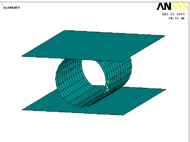
The whole meshing produced 288 Thin Shell elements with 360 nodes for the tube and 2 Thin Shell elements with total 8 nodes for the platens (Figure 1).

Fig 1. Meshed Mode

2.4 Contact Algorithms

In our modeling, we used the "Single Surface" contact with the setting to "Automatic" for all surface areas. This contact algorithm is the most general contact in LS-DYNA. It automatically detects if an external surface of a component contact itself or the external surface of another component. If penetration occurs, a penalty force is calculated between the contacting surfaces. This contact is chosen for the folding tube's surface, because it is the best one for crashing events, where the contact surfaces are not known in advance.

In addition, we use two "Node to Surface" contacts for the contacts between the platens and the tube. This is a fast and very efficient way to model a contact between known surfaces (i.e. tube and platen surface), because only the treatment for the node impacting the target is calculated. Because it is often used for modeling nodes that impact rigid bodies, we use it in our simulation, too. An additional benefit of this contact algorithm is the possibility to record the contact forces between "Contact" and "Target" in the "rcforce" ASCII output file. We will make use of this later, when the load carried by the tube is analyzed.

2.5 Load Application

In a transient dynamic analysis, loads must be defined for the duration of the analysis. To do so, arrays containing this data are created. For all loads a start and a stop time value are needed. The 1x2 array "TIME" sets the start time to zero and the stop time to one.

In the array "VELOCITY", the velocity of the moving platen is defined. The velocity curve is a straight line with constant velocity a. By using the known time value and the desired platen displacement s, the necessary final

velocity v can be calculated.

The displacement s was preset as 0.095 m. This represented the value of 0.95*D (95% of the original tube diameter) as given in Ref [1].

During the numerical simulations for the initial model calibration, we experienced, that a displacement of 0.95*D resulted in the total destruction of the tube, going along with a steadily increasing force between the platens, while the tube did not absorb any further energy. Because we found these results to distort the value for the cumulative absorbed energy, we decided to reduce the displacement to a value of 0.8*D throughout our following simulations. This value not only proofed to produce more reasonable results, but is also in accordance with our article Ref [1], which only says "up to 0.95*D" but does not use the same value of displacement throughout the experiments. For the comparison and interpretation of the results, of course, the experimental data will only be considered up to 0.8*D, too.

2.6 Boundary Conditions

We use the "Rigid" material to define the boundary conditions. The "Rigid" material offers the option to define rotational and translational boundary conditions for all parts that are meshed with the material "Rigid". Because we created two material models using the "Rigid" material (i.e. table and platen) we can easily define different boundary conditions for the two parts. For the table, we prohibit displacement in all translational directions and around every rotational axis. Because the upper platen is supposed to move in negative y-direction, we allow displacement upon the y-axis, but again prohibit every other displacement.

3. Results and Discussion

3.1 Simulation of quasi-static Crushing

For the simulation of the quasi-static crushing, all model parameters are set to the corresponding "quasi-static crushing" values. The goal is to validate the whole model by checking the model against the existing experimental values.

3.1.1 Initial Calibration

LS-DYNA is a complex FEM software with many parameters and dependencies among those parameters. Our goal was to produce a working model and achieve a realistic modeling behavior. The procedure was solving the model with the LS-DYNA solver and viewing the results in the LS-PREPOST post-processor. Doing this, visual comparison with the available experimental results allowed for a judgment on the quality of the model. Many improvements concerning element choice, contact algorithms and solution options could be made in this study phase.

A. Mahdi et al. [1] offered experimental developed results for a fiber-reinforced epoxy containing 3 identical segments of carbon shown in Fig 2. Those deformation histories were the guidelines to create an appropriate FEM model in ANSYS LS-DYNA. Fig 3 displays the results of our modeling work and allows a comparison with the given pictures from the former named article.

The authors pointed out that the failure mechanism "can vary from test to test even when all parameters are kept constant". Caused by this, the results of their crushing behavior tests represent the average of three tests. Since a computed model is not affected by a randomly varied material structure that influences the deformation,

there is only one result for our model. The development of the deformation process equals for our simulation and the experimental obtained results in big parts. One significant different is the behavior of the segments to each other. We wanted to use three different segments in our simulation, not only one. Due to this fact the contact of the segments to each other are simulated by friction. In reality those segments were embedded in epoxy. Caused by this it is obvious that the segments are divided after the shear forces are bigger than the friction that kept it together in the beginning. The Thin Shell elements presented in Fig 3 do not embody the geometric material properties. This means the thickness of the tube is mathematical respected and adjusted in the material properties but not displayed.

A significant flattening of the tubes at their contact point to the platen and table can be spotted in Fig 2 (a) and Fig 3 (e) / Fig 3 (f). On the left and the right side of the tube displayed in Fig 2 (e) develops a fracture line. The same kind of fracture is found on the right and left side of the tube in the computed model pictured in Figure 3 (h). After the flattening process of those parts that are in contact with table and platen follows a deformation towards the centre of the tube takes place. This is obvious in Fig 2 (c) / Fig 2 (d) as well as in Fig 3 (g) / Fig 3 (h).

in energy absorbed at the beginning of the crushing. However, in the second phase, the energy curve still has a parabolic shape. Worth to mention is that C-G-C and G-C-G tubes are converging to a common curve. The difference between them is not as high as one would expect, given the different material proportions. It seems like the segmentation alone has a more significant influence on the behavior of the tubes, than the ratio of the different materials.

In summary, we would recommend a C-C-C tube for highest SEA and a G-G-G tube for constant absorption behavior. A mixture of the two materials does not result in an improvement of the two characteristics.

4. Conclusions

In this paper, we presented an analysis on the total energy absorbed by laterally crushed composite tubes. The studies were conducted using an ANSYS LS-DYNA FEM model. The thematic of dynamic crushing is a complex area and the definition of the contact algorithms and material properties requires extreme care. To ensure consistency of the numerical data, we validated our modeling results using the experimental values given in Ref [2]. The results of the total energy absorbed and the experimentally developed values deviate only marginally. After verifying the behavior of the model, we extended the FEM simulation to dynamic crushing. The dynamic crushing simulation produced reasonable results for the total energy absorbed. We generated numerical data for different tube geometries (variation of the tube thickness t) and different tube segment materials (variation of the arrangement of glassfiber and carbon fiber composite segments, C-C-C/G-G-G/G-C-G/C-G-C).

The data shows that - for dynamic crushing situations – a thicker tube not necessarily yields a significantly higher SEA. For thin tubes, the additional mass compensates the improved load carrying capacity. However, for thicker tubes (t=3mm) the SEA improves clearly. On the other hand, a smooth linear progress of the SEA is favorable. This is given best for the thin tube (t=1mm). The analysis on the tube segment material shows that tubes with C-C-C configuration have the highest SEA, while tubes in G-G-G configuration show a smooth, constant absorption behavior.

This paper gives a draft for the modeling and analysis of the lateral crushing behavior of laterally loaded, segmented composite tubes. Further, comprehensive research is needed to underpin and extend the presented results. Particularly with regard to the dynamic crashing results, an examination with experimental developed data is desirable to confirm the numerical data in this paper.

Reference

[1] Zeng Tao, “Dynamic crashing and impact energy absorption of 3D braided composite tubes,” Elsevier, 2005.

[2] Mahdi Abosbaia, Sahari Hamouda and Mokhtar, “Energy absorption capability of laterally loaded segmented Composite Tubes,” Composite Structures, 2004.

[3] Herakovich Carl T., “Mechanics of Fibrous Composites,” Wiley, 1998. [4] Morgan Peter, “Carbon Fibres and their Composites,” CRC Press, 2005.

[5] Summerscales John, “Microstructural Characterization of Fibre-reinforced Composites,” CRC Press, 2001. [6] Livermore Software Technology Corporation , “Getting Started with LS-DYNA,” 2002.

[7] SAS IP, Inc., “Explicit Dynamics with ANSYS LS-DYNA,” 2003. [8] John O., “Hallquist – LS-DYNA Theory Manual,” 2006.