具有覆層為非線性之多層、多分支與多重量子井之平面型光波導結構之研究

行政院國家科學委員會專題研究計畫 成果報告

具有覆層為非線性之多層、多分支與多重量子井之平面型光

波導結構之研究

中 華 民 國 95 年 10 月 11 日

具有覆層為非線性之多層、多分支與多重量子井之平面型光

波導結構之研究

The Study of Multilayer, Multibranch, and

Multiple-Quantum-Well Planar Optical waveguide Structure

with Nonlinear Cladding

Abstract:

A novel method for analyzing the multilayer and multibranch planar optical waveguides with nonlinear cladding is presented. This method can also be used to analyze the multiple-quantum-well (MQW) waveguide structure. Numerical simulation results show that our analyses are reasonable.

中文摘要

我們提出一個分析覆層為非線性之多層與多分枝平面型光波導結構的新方 法，此方法亦可用來分析多重量子井光波導結構。數值分析的結果證明我們的分 析是正確的。

Key words: multilayer waveguide; multibranch waveguide; multiple-quantum-well

waveguide.

1. INTRODUCTION

In the past, the considerable interest has been raised in the theoretical and experimental study of optical properties of nonlinear interfaces. Until now, the published papers have dealt with structures where either a nonlinear film was sandwitched between both a linear substrate and cladding or two nonlinear films embedded among three linear media or a linear film was bounded by one or two nonlinear media [1-6]. Within the past several years, it became evident that multilayer systems as multiple quantum well structures exhibit the optical nonlinearities accompanied by very fast response time [7-10].

In the future, the multilayer and multibranch waveguide structures are very important components in application of integrated optics. The multilayer structures have been extensively used in the multiple-quantum-well waveguides [7-10] and the multibranch structures have also been designed to operate as all-optical photonic devices [11-16]. To the best of our knowledge, the general method for analyzing multilayer and multibranch waveguides with nonlinear cladding that is presented in this paper has not been reported before. Numerical results show that the method can also be used to

predict the evolution of a wave propagating in the nonlinear multibranch waveguide and to obtain electric field distribution of MQW waveguide.

2. ANALYSIS

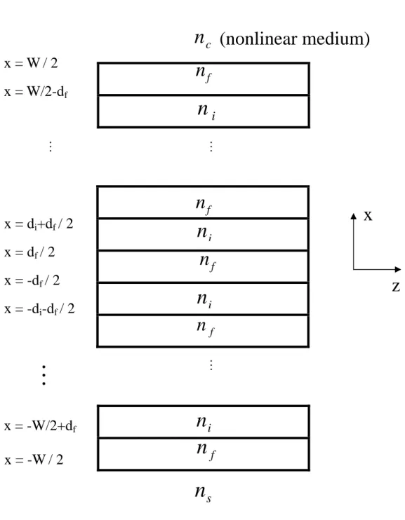
In this section, we use the basic electromagnetic theory [17] to derive the general formulae that can be used to analyze the multilayer and multibranch waveguides with nonlinear cladding, as shown in Fig.1. The multilayer structure is composed of guide films (n+1 layers), interaction layers (n layers), cladding, and substrate. The total number of layers is 2n+3 (n=0, 1, 2, ...). The cladding and substrate layers are assumed to extend to infinity in the +x and –x directions, respectively. The major significance of this assumption is that there are no reflections in the x direction to be concerned with, expect for those occurring at interfaces.

For the case of transverse electric (TE) polarized waves traveling in the z direction, the wave equation can be reduced to

2 2 2 2 2 j y y n c t ε ε ∂ ∇ = ∂ j=i, f, c, s (1)

with solutions of the form

0

( , , ) ( ) exp[ ( )]

y x z t E x i wt k z

ε = −β (2)

The subscripts i, f, c, and s in Eq. (1) are used to denote the interaction layer, guide film, cladding, and substrate, respectively. For TE waves, the electric field components ε_x and ε_z are zero. Note also in Eq. (2) that the transverse electric field has no y and z dependence because the planar layers are assumed to be infinite in these directions, precluding the possibility of reflections and resultant standing waves. In the following expressions of the field components, the time factor

( )

E x

(

)

exp and the z dependence exp

(

)

2

2 2

0

c c

n =n +α E (3)

where nc0 is the linear refractive index of the nonlinear medium and αis the nonlinear coefficient.

0 2 ( ) / cosh{ [ ( )]} c c c c E x q k q x x n α = − in the cladding (4) 0 ( ) ( ) cos{ [ ( )]} f f f f E x = A n k q x−x n in the film,β <n_f (5) 0 ( ) ( ) sinh{ [ ( )]} f f f f E x = A n k Q x−x n in the film,β >n_f (6) 0 ( ) ( ) cosh{ [ ( )]} i i i i E x =A n k q x−x n s

in the interaction layer (7)

( )

( )

(

)

s s

E x =A n k q x in the substrate (8)

The constants Q_f , q_c, q_i, q , and _s q_f can be expressed as 2 2 j j q = β −n j=c,i,s (9) 2 2 f f q = n −β β <n_f (10) 2 2 f f Q = β −n β >n_f (11)

By matching the boundary conditions, we obtain the following equations: 2

0

tan(k q d_{f f})=q q_f( _c+q_itanhΨ) /(q_f −q q_{c i}tanhΨ ) β <n_f (12) 2

0

tanh(k Q d_{f f})= −Q q_f( _c+q_itanhΨ) /(Q_f −q q_{c i}tanhΨ ) β >n_f (13) where Ψ can be expressed as

0 ( 1) [ 2 2 i i f i n n k q d − d x (1)] Ψ = + − (14)

The constants d_i and d_f are the widths of the interaction layer and the guide films, respectively. The transcendental equations (12) and (13) can be solved by numerical method on a computer. When the constant β is determined, all constants , , q_c q_i

f

q , Q_f , q , _s A_f(n), A (n), _s A_i(n), x (n), _c x_f (n) and x (n) are also determined _i

(appendix).

3. NUMERICAL RESULTS

In this section, we use the general formulae derived in the preceding section and in the appendix to calculate the transverse electric field functions in each layer of the multilayer nonlinear waveguide. Several numerical examples are presented as follows. When n=0, 1, 2, the general formulae can be simplified to analyze three-layer,

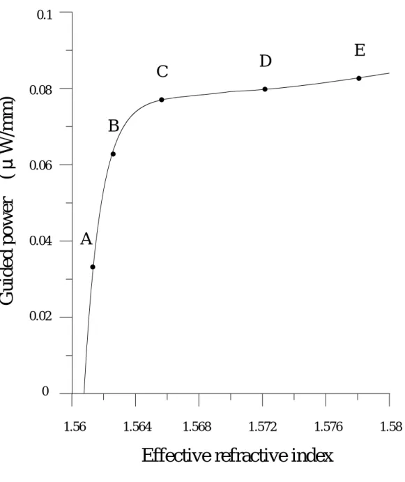
five-layer, and seven-layer nonlinear waveguides, respectively. The numerical results are shown in Fig. 2 to Fig. 7. Fig. 2 shows the dispersion curve of three-layer nonlinear waveguide with constants d_f =2µm , n_f =1.57, n =_s n_c0 =1.55,

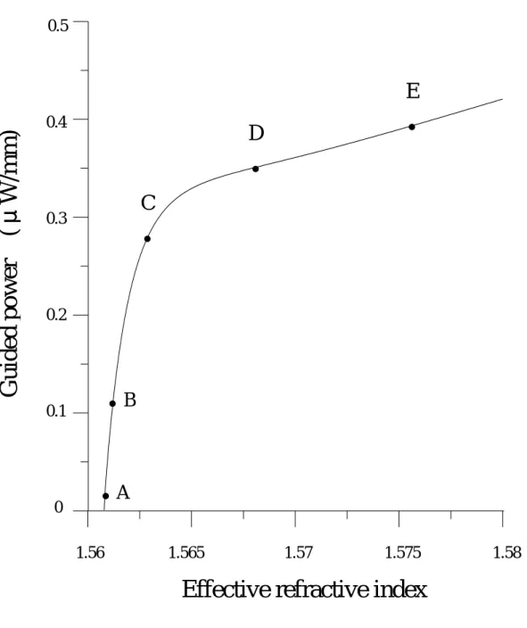
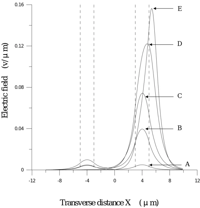
α=6.3786_µm2_/V2, λ=_{1.3 m}µ _{. Fig. 3 shows the electric field distributions for} several input powers, as shown in Fig. 2. Fig. 4 shows the dispersion curve of five-layer nonlinear waveguide with constants d_f =2µm, 6d_i = µm, n_f =1.57,

s

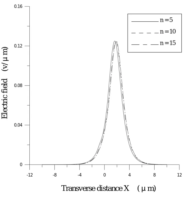
n =n_i=n_c0=1.55, α=6.3786µm2/V2, λ =1.3 mµ . Fig. 5 shows the electric field distributions for various input powers, as shown in Fig. 4. Fig. 6 and Fig. 7 show the dispersion curve and the corresponding electric field distributions of seven-layer waveguide, respectively. The parameters of seven-layer waveguide are the same as that of five-layer structure. As shown in Fig. 3, Fig. 5, and Fig. 7, as the guided power increases and consequently β increases, the field distributions gradually narrow, and the field maximum moves toward the linear-nonlinear boundary and then into the nonlinear medium. Now we consider a special case that the total thickness of the guide films and the interaction layers are confined to a value W, as shown in Fig. 8. Because the thickness of each guide film and each interaction layer is very thin, the number of layers just has a little influence on the electric field distributions. In this situation, multilayer waveguide likes a multiple-quantum-well waveguide. Fig. 9 displays the relations between n and the electric field distribution when the total thickness of the films and the interaction layers is 2 mµ by using general formulae.

Therefore, general formulae can also be used to analyze the MQW waveguide with nonlinear cladding.

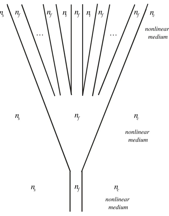
We can also use these general equations to analyze a multibranch waveguide with nonlinear cladding, as shown in Fig. 10. In the following analyses, the multibranch waveguide is divided into four sections: the straight waveguide section (the three-layer waveguide), the tapered waveguide section (the three-layer tapered waveguide), the coupled separating-waveguide section (the multilayer waveguide with the tapered interaction layer), and the isolated separating-waveguide section (the three-layer waveguides isolated from each other). The tapered-waveguide section and the separating-waveguide section can be approached by straight waveguide segments step by step[18-20]. These step-waveguide segments can be analyzed by the method proposed in the preceding section.

We can use this method to predict the evolution of a wave propagating along the multibranch waveguide from the stem to the branches. Here we show an example of a three-branch structure with nonlinear cladding, as shown in Fig.11. A concrete

example of application of the structure shown in Fig.11 is that this waveguide structure can be designed as a power-dependent all-optical switching device. The electric-field distributions of the four sections (positions , , , and as shown in Fig. 11) are shown in Fig. 12(a)-(d), respectively. In Fig.12(a), the electric-field distribution of the straight waveguide section is plotted with the constants 1 z z₂ z₃ z₄ m df =2µ , nf =1.57 , ns =nc0 =1.55 , β =1.561089943 , 2 2 6.3786 m V

α = µ , λ =1.3µm. In Fig. 12(b), the electric-field distribution of the tapered waveguide section is plotted with constants df =6µm, ns =nc0 =1.55,

066 727 567 . 1 =

β , α =6.3786µm2 V2 , λ=1.3µm. In Fig 12(c), the electric-field distribution of the coupled separating-waveguide section is plotted with constants

m

df =2µ , di =4µm , nf =1.57 , ni =ns =nc0 =1.55 , β =1.560 975 969 ,

2 2 6.3786 m V

α = µ , λ =1.3 mµ . In Fig. 12(d), the electric-field distribution of the

isolated separating-waveguide section is plotted with the constants

m

df =2µ , di =12µm , nf =1.57 , ni =ns =nc0 =1.55 , β =1.560 809 657 ,

2 2 6.3786 m V

α = µ , λ =1.3 mµ .

To prove the accuracy of the results shown in Fig. 12, we use the beam propagation method (BPM)[21] to simulate an eigenmode electric field propagating along the three-branch structure, from the stem to the branching waveguides. For the calculation, we choose the following numerical data: the transverse sampling points N=4096, a longitudinal step length ∆z =0.05µm , total propagation distance

m

Z =2200µ , the branching angle (shown in Fig. 11), the free space wavelength ° = 30. θ m µ

λ =1.3 , the nonlinear coefficient α =6.3786µm2 V2 , the suitable input power P0=0.367W/m, df =2µm, nf =1.57, and ni =ns =nc0 =1.55. The simulation result is shown in Fig. 13. By comparing the results shown in Fig. 12 and Fig. 13, we confirm that our analyses are reasonable.

4. CONCLUSIONS

We present a general method for analyzing the multilayer and multibranch waveguides with nonlinear cladding. This method can also be used to analyze the MQW waveguide structure with nonlinear cladding. We give a detailed modal analysis of nonlinear waveguide devices. The analytical results are accompanied by numerical examples. The numerical results show that our analyses are reasonable.

5.REFERENCES

1. A. D. Boardman and P. Egan, 1986, IEEE J. Quantum Electron. 22: 319. 2. C. T. Steaton, J. D. Valera, R. L. Shoemaker, G. I. Stegeman, J. T. Chilwell, and

D. Smith, 1985, IEEE J. Quantum Electron. 21: 774.

3. L. Leine, C. Wacher, U. Langbein, and F. Lederer, 1988, J. Opt. Soc. Amer. B 5: 547.

4. S. Ohke, Y. Satomura, T. Urneda, and Y. Cho, 1994, Japan J. Appl. Phys. 33: 3478.

5. T. Sakakibara and N. Okamoto, 1987, IEEE J. Quantum Electron. 23: 2084. 6. W. J. Tomlinson, 1980, Opt. Lett. 5: 323.

7. S. R. Cvetkovic and A. P. Zhao, 1993, J. Opt. Soc. Amer. B 10: 1401. 8. S. Selleri and M. Zobol, 1995, IEEE J. Quantum Electron. 31: 1785.

9. C. J. Hamilton, J. H. Marsh, D. C. Hutchings, J. S. Aitchison, G. T. Kennedy and W. Sibbett, 1996, Appl. Phys. Lett. 68: 3078.

10. C. Rigo, L. Gastaldi, D. Campi, L. Faustini, C. Coriasso, C. Cacciatore and D. Soldani, 1998, J. Crystal. Growth. 188: 317.

11. Y. D. Wu, M. H. Chen, and C. H. Chu, 2001, Fiber and Integrated Optics 20: 517.

12. M. H. Chen, and Y. D. Wu, 1992, Fiber and Integrated Optics 11: 395. 13. W. E. Martin, 1975, Appl. Phys. Lett. 26: 562.

14. T. J. Cullen, and C. D. Wilkinson, 1984, Opt. Lett. 9: 134. 15. Z. Weissman, E. Marom, and A. Hardy, 1989, Opt. Lett. l4: 293. 16. M. Izutsu, H. Haga, and T. Sueta, 1983, J. Lightwave Technol. 1: 285.

17. J. D. Jackson, 1975, Classical electrodynamics. New York: John Wiely and Sons 18. D. Marcuse, 1970, Bell Syst. J. 49: 273.

19. H. Yajima, 1978, IEEE J. Quantum Electron. 14: 749

20. W. K. Burns, and A. F. Milton, 1975, IEEE J. Quantum Electron. 11: 32. 21. Y. Chung, and N. Dagli, 1990, IEEE J. Quantum Electron. 26: 1335.

Appendix

The constants (n), (n), (n), (n), (n) and (n) can be expressed as follows： f A As Ai xc xf xi 1 0 1 1 ( 1) tanh ( 2 2 ) s f f i f f q n n x n d d k q q − + + = − − + (A1a) 1 0 1 1 ( 1) tanh ( 2 2 ) f f f i f s Q n n x n d d k Q q − + + = − − + − (A1b) 1 ( 1) 2 2 c f n n i x n+ = + d + d 1 0 0 1 1 tanh tan{ [ (1)]} 2 2 f f f i f c c q n n k q d d x k q q − ⎧ + ⎫ − _{⎨ ⎬} ⎩ + − ⎭ (A2a) 1 ( 1) 2 2 c f n n i x n+ = + d + d 1 0 0 1 1 tanh / tanh{ [ (1)]} 2 2 f c f f i f c n n Q q k q d d x k q − ⎧ + ⎫ + _⎨ + _⎬ ⎩ − ⎭ (A2b) 0 2 1 (1) / cosh{ [ ( 1)]} 2 2 f c c i f c n n A q k q d d x n α + ⎧ = _⎨ + − ⎩ + ⋅ 0 1 cos{ [ (1)]} 2 2 f i f f n n k q d + + d −x ⎫_⎬ ⎭ (A3a) 0 2 1 (1) / cosh{ [ ( 1)]} 2 2 f c c i f c n n A q k q d d x n α + ⎧ = _⎨ + − ⎩ + ⋅ 0 1 sinh{ [ (1)]} 2 2 f i f f n n k Q d + + d −x ⎫_⎬ ⎭ (A3b) 0 1 (1) (1) cos{ [ (1)]}/ 2 2 i f f i f f n n A =A k q d + − d −x )]} 1 ( 2 1 2 [ cosh{k₀q_i nd_i +n− d_f −x_i (A4a) 0 1 (1) (1) sinh{ [ (1)]}/ 2 2 i f f i f f n n A =A k Q d + − d −x

0 1 cosh{ [ (1)]} 2 2 i i f i n n k q d + − d −x (A4b) ， for 0≤ ≤ −p n 1 n− ≠p 1 0 2 3 ( ) ( 1) cosh{ [( ) ( ) 2 2 f i i i n n f A n− p = A n− −p k q − − p d + − − p d + 0 2 3 ( 1)]} / cos{ [( ) ( ) 2 2 i f i n n f x n− −p k q − − p d + − − p d } + ( )] f x n−p (A5a) 0 2 3 ( ) ( 1) cosh{ [( ) ( ) 2 2 f i i i n n f A n− p = A n− −p k q − −p d + − −p d + 0 2 3 ( 1)]}/ sinh{ [( ) ( ) 2 2 i f i f n n x n− −p k Q − −p d + − −p d + ( )]} f x n− p (A5b) for 0≤ ≤ − p n 1 0 2 1 ( ) ( ) cos{ [( ) ( ) 2 2 i f f i n n f A n−p =A n−p k q − − p d + − −p d + 0 2 1 ( )]}/ cosh{ [( ) ( ) 2 2 f i i n n f x n−p k q − −p d + − −p d + (A6a) )]}xi(n− p 0 2 1 h{ [(n ) (n ) ( ) ( ) sin 2 2 i f f i f A n−p =A n−p k Q − − p d + − −p d + 0 2 1 ( )]}/ cosh{ [( ) ( ) 2 2 f i i n n f x n−p k q − −p d + − −p d } + ( )] i x n−p (A6b) 0 1 [n n ( )]}/ k q d d x n ( 1) ( ) cosh{ 2 2 f i i i f i A n+ = A n + − + 0 1 cos{ [ ( 1)]} 2 2 f i f f n n k q d + − d +x n+ (A7a)

0 1 ( 1) ( ) cosh{ [ ( )]}/ A n n 2 2 f i i i f i n n A n k q d − d x + = − + + 0 1 sinh{ [ ( 1)]} 2 2 f i f f n n k Q d + − d +x n+ (A7b) 0 1 ( 1) cos{ [ ( 1)]}/ A A 2 2 s f f i f f n n n k q d + d x n = + + + + 0 1 exp[ ( )] 2 2 s i f n n k q d + d − + (A8a) 0 1 ( 1)]}/ f f n A A ( 1) sinh{ [ d x n 2 2 s f f i n n k Q d + = − + + + + 0 1 exp[ ( )] 2 2 s i f n n k q d + d − + (A8b) Ⅰ) n=even ( 0 1 2 n p ≤ ≤ − for 1 0 1 2 1 ( x ) ( ) ( ) tan 2 2 i f f i f f q n n n p p d p d k q q − ⎧− − − ⎪ − = − + + − + + _⎨ ⋅ ⎪⎩ 0 1 2 tanh{ [( ) ( ) ( )]} 2 2 i f i i n n k q − −p d + − −p d +x n− p ⎫_⎬ ⎭ (A9a) 1 0 1 2 1 ( ) ( ) ( ) tanh 2 2 / f f i f n n f x n p p d p d Q k Q − ⎧ − − − = − + + − + + _⎨ ⎩ 0 1 2 tanh{ [( ) ( ) ( )]} 2 2 i i f i i n n q k q − −p d + − −p d +x n−p ⎫_⎬ ⎭ (A9b) 1 0 1 1 ( ) ( ) ( ) tanh 2 2 f i f i i i q n n x n p p d p d k q q − ⎧− − − = − + + − + + _⎨ ⎩ ⋅ 0 1 tan{ [( ) ( ) ( 1)]} 2 2 f f i f n n k q − −p d + − p d +x n− +p ⎫_⎬ ⎭ (A10a)

1 0 1 1 ( ) ( ) ( ) tanh 2 2 i f i i n n / f x n p p d p d Q k q − ⎧ − − = − + + − + + _⎨ ⎩ 0 1 tanh{ [( ) ( ) ( 1)]} 2 2 i f f i f n n q k Q − −p d + − p d +x n− +p ⎫_⎬ ⎭ (A10b) for 1 2 n p n ≤ ≤ − 1 0 1 2 1 ( ) ( ) ( ) tan 2 2 i f f i f f q n n p p d p d k q q − ⎧ x n− = − − + + − − + − ⎪⎨− ⋅ ⎪⎩ 0 1 2 tanh{ [( ) ( ) ( )]} 2 2 i f i i n n k q − −p d + − −p d −x n−p ⎫_⎬ ⎭ (A11a) ⎩ ⎨ ⎧ − + − − + + − − = − − / tanh 1 ) 2 2 ( ) 2 1 ( ) ( 1 0 f f i f f Q Q k d p n d p n p n x 0 1 2 tanh{ [( ) ( ) ( )]} 2 2 i i f i i n n q k q − −p d + − −p d +x n−p ⎫_⎬ ⎭ (A11b) 1 0 1 1 ( ) ( ) ( ) tanh 2 2 f i f i i i q n n x n p p d p d k q q − ⎧− − − = − + + − + − _⎨ ⎩ 0 1 tan{ [ ( ) ( ) ( 1)]} 2 2 f f i f n n k q − − −p d − −p d −x n− +p ⎫_⎬ ⎭ (A12a) 1 0 1 1 ( ) ( ) ( ) tanh / 2 2 i f i i n n f x n p p d p d Q k q − ⎧ − − = − + + − + − _⎨ ⎩ 0 1 tanh{ [ ( ) ( ) ( 1)]} 2 2 i f f i f n n q k Q − − −p d − −p d −x n− +p ⎫_⎬ ⎭ (A12b) (Ⅱ) n=odd r fo 0 3 2 n p − ≤ ≤ 1 0 1 2 1 ( ) f x n p ( ) ( ) tan 2 2 i f i f f q n n p d p d k q q − ⎧ − − − ⎪ − + + − + + _⎨ ⋅ ⎪⎩ − =

0 1 2 tanh{ [( ) ( ) ( )]} 2 2 i f i i n n k q − −p d + − −p d +x n− p ⎫_⎬ ⎭ (A13a) 1 0 1 2 1 ( ) ( ) ( ) tanh 2 2 / f f i f n n f x n p p d p d Q k Q − ⎧ − − − = − + + − + + _⎨ ⎩ 0 1 2 tanh{ [( ) ( ) ( )]} 2 2 i i f i i n n q k q − −p d + − −p d +x n−p ⎫_⎬ (A13b) ⎭ 1 0 1 1 ( ) ( ) ( ) tanh 2 2 f i f i i i q n n x n p p d p d k q q − ⎧− − − = − + + − + + _⎨ ⎩ ⋅ 0 1 tan{ [( ) ( ) ( 1)]} 2 2 f f i f n n k q − −p d + − p d +x n− +p ⎫_⎬ ⎭ (A14a) 1 0 1 1 ( ) ( ) ( ) tanh 2 2 i f i i n n f x n p p d p d Q k q − ⎧ − − = − + + − + + _⎨ ⎩ / 0 1 tanh{ [( ) ( ) ( 1)]} 2 2 i f f i f n n q k Q − −p d + − p d +x n− +p ⎫_⎬ ⎭ (A14b) r 1 1 2 n p n + _{≤ ≤ −} fo 1 0 1 2 1 ( ) ( ) ( ) tan 2 2 i f f i f f q n n x n p p d p d k q q − ⎧− − − ⎪ − = − + + − + − _⎨ ⎪⎩ ⋅ 0 1 2 tanh{ [( ) ( ) ( )]} 2 2 i f i i n n k q − −p d + − −p d −x n−p ⎫_⎬ ⎭ (A15a) 1 0 1 2 1 ( ) ( ) ( ) tanh 2 2 / f f i f n n f x n p p d p d Q k Q − ⎧ − − − = − + + − + − _⎨ ⎩ ⎭ ⎬ ⎫ − + − − + − − )]} ( ) 2 2 ( ) 2 1 [( tanh{k₀q n p d n p d x n p q_{i i f i i} (A15b) 1 0 1 1 ( ) ( ) ( ) tanh 2 2 f i f i i i q n n x n p p d p d k q q − ⎧− − − = − + + − + − _⎨ ⎩ ⋅

0 1 tan{ [ ( ) ( ) ( 1)]} 2 2 f f i f n n k q − − −p d − −p d −x n− +p ⎫_⎬ ⎭ (A16a) 1 0 1 1 ( ) ( ) ( ) tanh 2 2 i f i i n n / f x n p p d p d Q k q − ⎧ − − = − + + − + − _⎨ ⎩ 0 1 tanh{ [ ( ) ( ) ( 1)]} 2 2 i f f i f n n q k Q − − −p d − −p d −x n− +p ⎫_⎬ ⎭ (A16b) otherwise 1 0 0 1 1 1 1 1 ( ) tan tanh{ [ ( )]} 2 2 2 2 2 2 i f i i i i f f q n n x d k q d x k q q − ⎧ ₋ ⎫ ⎪ ⎪ + = − _⎨ − + _⎬ ⎪ ⎪ ⎩ ⎭ (A17a) 1 0 0 1 1 1 1 1 ( ) tanh / tanh{ [ ( )]} 2 2 2 2 2 2 f i f i i i i f n n x d Q q k q d x k Q − ⎧ ⎫ + = − _⎨ − + _⎬ ⎩ ⎭ (A17b) 1 0 0 1 1 1 1 3 ( ) 2 2 i n n x + = − tanh tan{ [ ( )]} 2 2 2 2 f i f i f i i q d k q d x k q q − ⎧− ⎫ + _⎨ + + _⎬ ⎩ ⎭ (A18a) 1 0 0 1 1 1 1 3 ( ) tanh / tanh{ [ ( )]} 2 2 2 2 2 2 i i f i f i f i n n x d Q q k Q d x k q − ⎧ ⎫ + = − + _⎨ + + _⎬ ⎩ ⎭ (A18b)

… … c

n

(nonlinear medium)

n

n

n

n

n

n

n

n

n

n

.

.

.

x = d

/ 2

x = -d

/ 2

x = -d

-d

/ 2

x = d

+d

/ 2

x

z

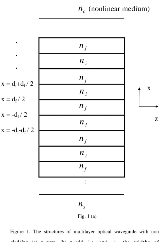
Figure 1. The structures of multilayer optical waveguide with nonlinear cladding (a) n=even, (b) n=odd, ( and the widths of the interaction layer and the guide films, respectively).

i

… … c

n

(nonlinear medium)

n

n

n

n

n

n

n

n

n

n

.

.

.

.

.

.

x = d

/ 2

x = -d

/ 2

x = -d

-d

/ 2

x = d

+d

/ 2

x

z

0.0001

A

B

C

D

E

Figure 2. Dispersion curve of the three-layer optical waveguide structure with nonlinear cladding.

G

u

id

ed

p

o

w

er

(μ

W

/m

m

)

Effective refractive index

1.56 1.564 1.568 1.572 1.576 1.58 0.1 0.08 0.06 0.04 0.02 0

C

Electric

field (v/

μ

m)

E

D

B

A

Transverse distance X (μm)

Figure 3. The electric field distributions with respect to A、B、C、D、E five points as shown in figure 2, (x=0 representing the symmetric center of the structure).

0.0003 0.0004 0.0005

Guided

power (

μ

W/mm)

A

B

C

D

E

Figure 4. Dispersion curve of the five-layer optical waveguide structure with nonlinear cladding.

Effective refractive index

A

C

E

Electric

field (v/

μ

m)

D

B

Transverse distance X (μm)

Figure 5. The electric field distributions with respect to A、B、C、D、E five points as shown in figure 4, (x=0 representing the symmetric center of the structure).

0 0.0001 0.0002 0.0003 0.0004 0.0005 ●

A

B

C

D

E

Figure 6. Dispersion curve of the seven-layer optical waveguide structure with nonlinear cladding.

G

u

id

ed

p

o

w

er

(μ

W

/m

m

)

Effective refractive index

C -20 -10 0 10 20 0 0.04 0.08 0.12

E

Electric

field (v/

μ

m)

D

A

C

B

Transverse distance X (μm)

Figure 7. The electric field distributions with respect to A、B、C、D、E five points as shown in figure 6, (x=0 representing the symmetric center of the structure).

c

n

(nonlinear medium)

n

n

n

n

n

z

n

n

n

n

n

n

x = d

+d

/ 2

x = -d

/ 2

x = d

/ 2

x = W/2-d

x = W

/ 2

x

x = -d

-d

/ 2

…

x = -W/2+d

x = -W

/ 2

Figure 8. Schematic diagram of a multiple-quantum-well waveguide structure with nonlinear cladding.

-12 -8 -4 0 4 8 12 0 0.04 0.08 0.12 0.16

n = 5

n = 10

n = 15

Electric

field (v/

μ

m)

Transverse distance X (μm)

Figure 9. The electric field distribution of the multilayer waveguide with MQW structure(W=2μm).

f

n

n

n

n

n

n

n

n

n

n

n

n

n

nonlinear

medium

…

…

n

n

n

nonlinear

medium

n

n

nonlinear

medium

Figure 10. The structure of a multibranch waveguide with nonlinear cladding.

Z

….

Z

….

Z

………..

Z

………

Z

………..

n

n

n

n

n

n

n

n

nonlinear

medium

nonlinear

medium

n

n

n

n

n

nonlinear

medium

Figure 11. The structures of a 1×3 three-branch waveguide with nonlinear cladding.

-20 -10 0 10 20 0 0.02 0.04 0.06 0.08 -20 -10 0 10 20 0 0.02 0.04 0.06

Electric

field (v/

μ

m)

Electric

field (v/

μ

m)

Transverse distance X

Transverse distance X

(a) (b) -20 -10 0 10 20 0 0.01 0.02 0.03 0.04 0.05 -20 -10 0 10 20 0 0.02 0.04 0.06

Electric

field (v/

μ

m)

Electric

field (v/

μ

m)

Transverse distance X

Transverse distance X

Figure 12. The electric field distributions of the four sections of the three-branch waveguide with nonlinear cladding : (a) at the straight waveguide section (position Z1); (b) at the tapered waveguide section (position Z2); (c) at the

coupled separating-waveguide section (position Z3); (d) at the isolated

P ro p ag at io n D is ta n ce Z ( m ic ro n )

P

ro

p

ag

at

io

n

D

is

ta

n

ce

Z

(

m

ic

ro

n

)

Propagation Distance Z (micron)

-20 -10 0 10 20 0 200 400 600 800 1000 1200 1400 1600 1800 2000 2200 Z4=2200μm

Propagation Distance Z

(μ

m)

Transverse Distance X

(μm)

Figure 13. The evolution of an electric field propagating along the three-branch waveguide structure with nonlinear cladding.