Quantum transport through a quantum well in the presence of a finite-range time-modulated potential

CHINESE JOURKAL OF PHYSICS VOL. 37, NO. 5 OCTOBER 1999

Quantum Transport Through A Quantum Well in the Presence of a Finite-Range Time-Modulated Potential

C. S. Chu and H. C. Liang

Department of Electrophysics, National Chiao Tung University, Hsinchu, Tazwan 300, R.O.C.

(Received March 5, 1999)

We have studied the transport of electrons through a quantum well within which a time-modulated potential of amplitude Vz, range a, and frequency w is applied. Our results show that, as the chemical potential p increases, the dc conductance G exhibits Fano-structures when p is at mhw above the bound state energy in the well. As Vz increases, the Fano-structures are broadened, and higher rnfiw processes emerge. These features are identified as the formation of quasi-bound states. For a fixed but large potential strength VI = aVz, the Fano-structures are broadened and are shifted toward lower electron energies, as a decreases. The dependence of the Fano-structure to the location of the time-modulated potential is also studied.

PACS. 72.10.-d - Theory of electronic transport; scattering mechanisms. PACS. 72.4O.+w - Photoconduction and photovoltaic effects.

PACS. 73.40.-c - Electronic transport in interface structures.

I . I n t r o d u c t i o n

Inelastic scatterings are very important for the quantum transport in nanostructures because they give rise to characteristics that reflect the energy spectrum in the structures. .4 systematic exploration is possible when a time-modulated potential is induced over a certain region of the structures [l-lo].

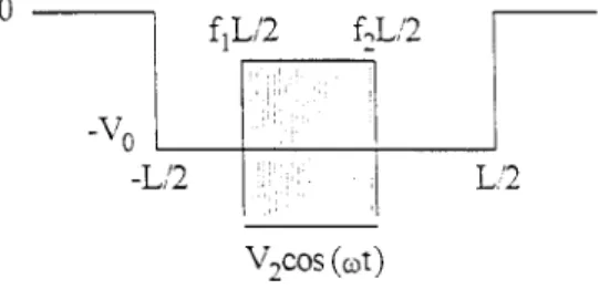
The nanostructures we consider consist of a quantum well in the middle of a narrow constriction (NC) which is acted upon by a time-modulated gate-potential, as shown in Fig. 1. Similar configurations have been investigated by Tang and Chu [9], except that the NC did not consist of a quantum well. Their focus was on the resonance conditions when the incident electron energies are at mtiw above the threshold energy of a subband in an NC. However, the presence of a quantum well opens up discrete levels below the original threshold energies. How these discrete levels affect the resonance conditions is the issue we investigate in this work. Recent developments in the split-gate technology have made possible the fabrication of such gate-controlled quantum point contacts (&PCs) [ll], and thus it is possible to investigate the resonance conditions in NC that has discrete levels below the threshold energies, and is acted upon by a time-modulated potential.

509 @ 1999 THE PHYSICAL SOCIETY OF THE REPUBLIC OF CHINA

v,cos

(at)

FIG. 1. Sketch of a quantum well structure with a time-modulated potential in between the edges of the quantum well.

In reference [9], the dip structures in the dc conductance G are closely related to the density of states (DOS) in the NC. The energy levels in the NC are quantized into one-dimensional subbands so that the DOS is singular at the subband bottoms. This allows the quasi-bound-states at energy just below a subband bottom to be induced by the time-modulated potential. The dip or peak structures in G occur whenever p is of mfLw above a subband edge. These are the quasi-bound-state features, which is associated with the situation when the electrons can make transitions, via inelastic processes, to the quasi-bound-states. It is important to ask whether such quasi-bound-state features in G could _ persist in the case when discrete levels exist below the subband edges. Such situation can

be realized by adding a quantum well structure in the NC.

In this paper, we extend the work of references [9] and [12] by allowing a time-modulated potential to act upon the quantum well structure. The abruptness in the profile of both the quantum well and the time-modulated potential has caused additional multiple scatterings, which result in harmonic structures in G [9]. In reference [9], the harmonic structures in G due to the finite-range time-modulated potential are obvious. But with the presence of a quantum well, we find that the harmonic structures are dominated by multiple scatterings between the length of the quantum well.

The finiteness in the range of the time-modulated potential also made possible the intra-subband and the inter-side-band transitions for the transmitting electrons. This is due to the breaking of the longitudinal translational invariance in the NC. Furthermore, we have taken that the lengths of the quantum well and the time-modulated potential are less than the phase-breaking length 14. By this the entire transmission process through the structure is coherent. The two reservoirs at both ends of the NC are free from the time-modulated effects so that the distribution of the incident electrons is well determined. Thus the description of the quantum transport follows the Landauer-Biittiker-type formalism.

In Sec. II we present the formulation for the scattering and the connection of the transmission coefficients with the conductance G. In Sec. III we present numerical exam-ples illustrating the quasi-bound-state features in a finite-range time-modulated potential. Finally, Sec. IV presents a conclusion.

II. Theory

trans-VOL.37 C.S. CHU AND H. C.LIANG 511

mission and reflection coefficients are obtained. The conductance G is then expressed in terms of these coefficients.

The QPC is modeled by a NC connected adiabatically at each end to a 2DEG such that the transmission of the electrons into or out of the NC is adiabatic [13]. The time-modulated potential is within the quantum well and does not affect the reservoirs outside the quantum well. The NC is taken to have a quadratic transverse confinement, given by the potential 2mzw,y .2 2 The potential of the quantum well system takes the form

V(xJ) =

-v,e

( 1

g -

1x1 +

v,

cos(wt)8

(x-~)e($-x).

(f2 - f&5/2 - a with -1 5 fr 2 f2 5 1, and z is the transmission direction.

Choosing the energy unit E* = h2kg/2mz, the length unit a* = l/lc~, the time unit t* = h/E*, I+ and V2 in units of E’, the dimensionless Schrodinger equation becomes

I--

v2

+w;y2

+

V(x,t)]q5,t) =

i$(ZJ).

(2)

Here kF is a typical Fermi wave vector of the reservoir and rn: is the effective electron mass. The transverse energy levels are quantized, with energy Ed = (2n - l)w, and wave function &(y), where n is a positive integer excluding zero. The quantum well and the time-modulated potential are uniform in the transverse direction and do not induce inter-subband transitions, leaving the inter-subband index n unchanged. Thus for an nth inter-subband electron incident along 2 and with energy p, the scattering wave function can be written in the form q$(Z,t) = &(y)$+(~,t) [7,10], where

ei~n,o (Z-t $)e-ipt +

CTn,,e

-ik,,,(l-+~)e-i(,+m,)t > m 5 < - L / 2 C[A~,,e'qn~m(z+$) +

B~,me-iq,,,(r+~)]e-i(~+~~)~,

m - L / 2 < 2 < fiL/2

~[Jp(VZ/w)e-iPWt]

CIC,,,teiqnlm'z

+

D,,m,e-iq”,,f~]e-i(CL+m’w)t,

P m’ (3)

fd/2 -c

x < f2LJ2 C[A~,,e-iq~~m(z-$) + B~,meiq”,,(r-~)]e-i(~+~~)~, m f2L/2 < 2 < L / 2 C tn,meik,77t(z-$)e-i(p+mw)t > L/2 < 2, m

and n,m are the final subband and side-band indices, respectively. The effective wave vector for electrons with incident energy E and in the nth subband is given by k,,, =

E - (2n - l)w, + mw, and q12,m = E + VO - (2n - l)w, + mw. The sideband index m corresponds to the net energy change of mIiw for the outgoing electrons.

The expressions for the reflection and transmission coefficients can be obtained from matching at the four edges of the quantum well and the time-modulated potential. matching conditions are required to hold in all times.

After performing the matching at 2 = &L/2, we obtain

T_{n,m =} 2Ak,mqn,m - 6m,o(qn,m + kn,m) - kn,m 7 4n,m B’ =_n,m AL,, (qn,m + k,m) 4n,m - kn,m ’

t

n,m

=

2-4,m qn,m

4n,m

-

kn,m'

After performing the matching at z = frL/2, we obtain

Ai,m

eiqn,m(fl+l)$ +

e-iqn,,(fl+l)l.

4

Qn,m

+

kn,m)

_

26

kn,me-“q-(fi+l)$

(Qn,m -

kn,m)

1

m’o

(qn,m - kn,m) =

c[

Cn,n’I+dl

c +

Dn,n,e-%,rfl

$

n’

] Jm-n!(z),

Ah,m

eiqn,m(fl+l)$ _

e-iqn,,(fl+l)T

4

Qn,m

+ kn,m> +

26

iq”,m(fl+l)~ - kn,m)₁ m

’

(qn2m;

“1 (V*) o

kn,me-(Sri,,, - kn,m) =

c

E

[cn,nteiqn.nrjl+ -

Dn,n,e-*qn,n’ 17 J,_,, w . n’ ’

After performing the matching at z = fzL/2, we obtain

-h,m(fi-l)$ +

eiqn,m(f2-1),

4

4n,m + kn,m) n,m - kn,m) 1 = XIc+eiqdf2$ + Dn,n,e-i%,,n’f2$ J,_,, 3 n’ (Rj 0w ’ AL,m9n,m -e [ -iqn,m(.fi-I)$ + eiqn,m(fz-1)24 4n,m + kn,m) (Qn,m - kn,m)₁ = xqn,n, [Cn,n,eiqn,nrf2$ _ Dn,n,e-iqn,nlfz$ n’ ] Jm-nl (z) . The (4) (5) (6) (7) (8) (9)

(11)

VOL.37 C.S. CHU AND H. C.LIANG 513

G = y

c e,tn,_,2,

R.7n 1

where n,m include only the propagating modes whose

k,,,

is real. The factor of 2 is due to the spin degeneracy.

Solving Eqs. (8)-(ll), we obtain

A',,,, A;,,, C,,,,

and D,,,. We then obtain T,,, and t,,, by Eqs. (5) and (7).

We solve the coefficients T~,~ an d t,,, exactly, in the numerical sense, by imposing a large enough cutoff to the side-band index. The correctness of our procedure is checked by a conservation of current condition, given by

(13)

where m includes again only the propagating modes. We have also checked that G is converged for our choice of the side-band cutoff.

III. Numerical results

In this section, we present numerical examples for the conductance G as a function of the chemical potential p. Since each occupied subband contributes independently to G, it suffices for our purpose here to present the conductance of only one subband, which we take to be the lowest one.

Besides p, G depends also on L,

Vo, a, VZ, w,

and the position of the time-modulated potential. The unperturbed bound state energies are determined by

L

and

Vo;

the side-band separation is w; aV2 is the strength of the time-modulated potential; and its position (center) (f2 + f1)L/:! det ermines the shape of the quasi-bound-state structures in G. We present these G behaviors in five situations. First, G is shown for a NC that do not have a quantum well

(Vo = 0),

with a fixed

a

and w, while varying

Vz.

Second, G is shown for fixed L = a,

Vz

and w, while varying the depth of the quantum well

Vo.

Third, G is shown for different frequencies w with fixed

Vo, Vz

and

L = a.

The fourth situation is to compare G for fixed

VO, L, w

and the strength of the time-modulated potential aV2, while varying a. Finally, we present

G

for fixed

Vo, VZ, L, a,

and w, while varying the position of the time-modulated potential (j2 + fi)/2.

In our numerical examples, the NC is taken to be that in a high-mobility GaAs-Al,Gai_,As with a typical electron density w 2.5 x 10” cmF2 and rnz = O.O67m,. Cor-respondingly, we choose an energy unit

E' = fL2k~/(2m,") = 9

meV, a length unit a* =

l/kF = 79.6 .&,

and a frequency unit w+ =

E*/h =

13.6 THz. We also take wy = 0.035, such that the effective NC width is of the order of lo3 A. In the following, in presenting the dependence of G on CL, it is more convenient to plot G as a function of X instead, where

X = [(/.&)t 1]/2.

The integral value of X is the number of propagating channels. In Fig. 2,

G

is plotted against X for a NC structure acted upon by a time-modulated potential. There is no quantum well, with

V, = 0.

The time-modulated potential has a = 12, w = 0.014, and V2 = 0.003, 0.012, and 0.024. The energy interval w corresponds to an interval AX = w/(2wY) = 0.2 on the ordinate. At X = 1, the chemical potential

y is at the subband edge. We note that a major dip structure occurs at X = 1.2, which corresponds to X - AX = 1. This is a quasi-bound-state feature because the electron with energy X can make transitions to the quasi-bound-state just beneath the subband edge by giving up an energy w. In general, for larger Vz, the structures of more photon processes at X = 1 + mAX are more evident. This is the situation when the electrons can emit energy

of mw and make transitions to the quasi-bound-state beneath the subband edge.

We note here that the structures in G induced by the time-modulated potential do not always carry the dip structure characteristics. In general, these are cases of Fano-resonance form [5,14-161. The origin of the Fano-Fano-resonance is due to the existence of a quasi-bound-state imbedded in a continuum. In fact, this quasi-bound state in a NC can be shown to have a small negative imaginary part in energy, and is evanescent in space [17]. Detail discussions are presented in the appendix. If there were no inelastic scattering, the quasi-bound-states would not couple to a continuum. But in the presence of the inelastic scatterings, the quasi-bound-state just below the 72th subband threshold energy Ed can be coupled to the states E~ + mw, which are certainly embedded within a continuum. Thus it is not surprising to find Fano-structures in G. The form of these Fano-structures are pairs of neighboring peak and dip structures. Their detail shape, however, can change gradually, such as those in Fig. 2, and also in Fig. 4 of reference [15], where the dip is smeared or is diminished for larger interaction strength. But in our case here, such as that in Fig. 2 and in Fig. 6, the Fano-structures exhibit even more drastic change.

The wavelength of the incident electron decreases as X increases. The relation is given by X = 2=/\/2wy(x--1). At the energy with subband index n = 1, when X = 1.2, we have X = 53. Thus, near the first resonance, the range of the time-modulated potential is short, with a 2: 0.23X.

In Fig. 3, G is plotted against X for L = a = 12, such that the position (center) of the time-modulated potential is at 2 = 0. Other physical parameters are V, = 0.012,

w = 0.014, and Vo = 0.0077, 0.0153, 0.0230. To understand the correlation of the structures

in G with the bound states in the well, we write down the confining equations for the bound states with energy Eb (Eb < 0) in the case when Vz = 0. For even parity bound states, the equation is

and for odd parity bound

tan

[~&iijTFj]

m

-Jm=O;

states it is

(14)

where F = Eb/Vo. Again, because of the inelastic scattering, the unperturbed bound states in the quantum well are coupled with the states with energies _?$, + mw > 0. These coupling are found to give rise to Fano-structures in G and at XL values given by

xi=

1-t VoF + mw2w .

VOL.37 C.S. CHU AND H. C.LIANG 0.6 -= 3 # 0.6 -D a =12 y: .Z= OL-5 - \‘2=o.oo3 3 0.2 -0.6 FIG. 2. : 0 : .2 TL 1 6 78 2 0 X

Conductance G as a function of X for a NC structure acted upon by a time-modulated potential. The width of the time-modulated potential a = 12, w = 0.014, and V2 = 0.003, 0.012, and 0.024. The dip structures at X = 1.2 are due to the situation when the electrons, after giving away energy w, make transitions to the quasi-bound-states below a subband edge. For larger Vz, the quasi-bound states are more broadened and many-photon processes at X = 1 + mAX, with AX = 0.2, are more evident.

515 L=a= 12 - v. = 0.0077 -.-.-v, = 0.0153 .___..___.. v. = 0.0230 1 06 FIG. 3. '1.0 1.2 '14 1.6 1.6 2.0 X Conductance G as a function of X for a quantum well structure acted upon by a time-modulated potential. The width of the time-modulated po-tential a = 12 is equal to the well width L, Vz = 0.012 and w = 0.014. The well depth VO are 0.0077, 0.0153, and 0.0230. The Fano-structures be-fore X = 1.2 are due to the situa-tion when the electrons, after giving away energy w, make a transition to an originally bound state. The struc-tures between X = 1.2 and X = 1.4 are due to the situation when the electrons, after giving away energy 2w, make transitions to the originally bound state.

The evaluated (Xp , X,“) are (1.178, 1.378), (1.128, 1.328), (1.065, 1.265), for Vo = 0.0077, 0.0153, 0.0230 respectively. The close correspondence between the evaluated Xk values and the Fano-structures in Fig. 3 demonstrates that the singular DOS at the unper-turbed bound state energies inside the well does play an important role. In addition, our other results show that the Xh locations shift to smaller values for larger aV, while the Fano-structures are broadened. This can be understood as the broadening of the bound state energies by the strength aVz of the time-modulated potential.

In Fig. 4, G is plotted against X for L = a = 12, such that the position of the time-modulated potential is at 5 = 0, VZ = 0.012, Vi = 0.0230, with w = (0.014, 0.028, 0.042), respectively. The corresponding Xis are (1.065, 1.265, 1.465), and they correspond closely to the Fano-structures. At X,b, the electron wavelength Xs are (93.0, 37.6, 30.7). Thus, a N (0.13X, 0.31X, 0.39X), in each case.

In Fig. 5, G is plotted against X for 1 2 , w = aV. =

L=a=lZ - 0=0.014 -.-.- 0 = O.fJ28 __._._ _ ._.. o = o&Q 0.8 FIG. 4.

I

10 3.2 7 4 1 6 i 6 2 0 X

Conductance G as a function of X for a quantum well structure acted upon by a time-modulated potential. The width of the time-modulated poten-tial a = 12 is equal to the well width L, Vz = 0.012 and Vo = 0.0230. The frequencies w are 0.014, 0.028, and 0.042. The energy differences of the resonant structures are multiples of 0.014.

FIG. 5. Conductance G as a function of X for a quantum well structure acted upon by a time-modulated potential. L = 12, aV2 = 0.144 and VO = 0.0230, w = 0.014,

f2 + fi =

0, such that the position of the time-modulated po-tential is at the center of the quan-tum well. The width of the time-modulated potential a are 12, 6, and 3. These curves show the same form of a quasi-bound-state structure with broadened resonance for thinner a. coincides with the center of the well. These curves correspond to the same resonance energy Xt = 1.065 and are of similar Fano-resonance form. As a decreases, the Fano-structures shift toward lower energies and the structures are more broadened. Our other results show that for a fixed but smaller a& value, the electrons can not make transitions to the bound state in the well except when their energies are very close to Eb + hw.

In Fig. 6, G is plotted against X for L = 12, a = 3, w = 0.014, V, = 0 . 0 2 3 0 ,

V, = 0.012, while varying the position (f2 + fi)L/2 of the time-modulated potential inside the well. These curves show that the resonance form is position dependent and is symmetric with respect to the position of the quantum well, as is shown by the exact overlap of the two curves for (f2 + fi)/2 = f0.25.

IV. Conclusion

We have solved nonperturbatively the quantum transport in a NC that consists of a quantum well and a time-modulated potential. The scattering process is both coherent and inelastic. We find that the bound states in the well become quasi-bound in the presence of a time-modulated potential. Besides the broadening of the bound state energies, the bound state energies are shifted to lower values and more importantly, they are coupled to the states & + mw > 0 in a continuum. Thus, G exhibits Fano-structures.

VOL. 37 C.S. CHU AND H. C. LIANG 517 FIG. 6 1.0 -cry r,, ‘2 =

i!.\

0.8-

-

-01s _\ 3 -.-.- 0.W \ 201 _.__... 035 2 06 - /__--.--:.:~ 0

..-,;_1

“i.. --.-0.50 __(, . ..I..: v. .I: -...- 0.75 = OL- /.:-.=--‘~ ., _..-5-y \ !,,/ 2 . . r. ‘Q:;, 0.2 : : \! 00 -L=E:a=X I,, i! , 1 , ,_ 103 i0.c : 05 1.06 T.07 1 oe X

Conductance G as a function of X for a quantum well structure acted upon by a time-modulated potential. L = 12, a = 3, w = 0.014, well depth Vo =

V-2 = 0.012. The positions of the time-modulated potential corresponding to (fi + fi)/2 are -0.25, 0, 0.25, 0.5, and 0.75. These curves show that the conductance G, as a function of the position of the time-modulated potential, is symmetric with respect to the location of the quantum well.

From the results we have not shown here, we find that in a one-side-band approxima-tion [12,18], the G values are, in general, quite different from the exact results, even though the results satisfy the conservation of current condition quite reasonably. In fact, perturba-tion method with the one-side-band approximaperturba-tion is valid only when the strength aV.2 is very small. For most cases of interest, we have to go beyond one-side-band approximation. For clarity, we have chosen the parameters of the quantum well such that there is only one unperturbed bound state inside the quantum well. This approach can be easily generalized to cases that have more bound states, with qualitatively similar results expected.

A c k n o w l e d g e m e n t s

This work was partially supported by the National Science Council of the Republic of China through Contract No. NSC 88-2112-M-009-028.

A P P E N D I X : DOS argument about quasi-bound state

The existence of the quasi-bound state in a NC, be they impurity-induced or oscillating-barrier-induced, is more a characteristics of the NC than the way they are being induced. Detail discussions have been given by Bagwell and Lake in reference [5]. In the following, we supplement by presenting a DOS argument as in reference [17], and extend this argument into a quantum well system. The DOS in a NC is given by p(S; E) = -ImG’(S, Z; ,3)/n, Ghereljin our choice of units, the retarded Green’s function G’(Z,Z’; E) = C,[#~~(y)&(y’)/

26, eznnlz-Z 1. Here K n = d=, and n is the subband index. It is clear from the DOS expression that for E just below EN, the subband N does not contribute to the DOS. I n addition, the wavefunction for this energy E and in this subband iV is evanescent a l o n g

the longitudinal direction. However, if we allow E to be analytically continued into the lower half complex energy plane, such that E = Ed - 6E - iE;, the contribution of the subband N to the DOS becomes [&(y)/2x][6E2 + E;2]-1/4 sin[(l/a)tan-l(Ei/sE)], which, when 6E N E; N 0, can be very large. And the factor e -iEt decays with time. So there is a locally bound state with lifetime at this energy. This wavefunction will decay and go away from propagating channels. So the quasi-bound state can happen at the subband bottom with N > 1 under time-dependent perturbation. And, under coherent inelastic scattering, the quasi-bound state can also happen at the first subband bottom because there are some propagating states that couple to this energy.

In the presence of a quantum well, the DOS is still given by p(Z; E) = -ImG’(Z, 37; E)/

Thyhere,

&

the retarded Green’s function G’(Z,Z’; E) = Cn,,l~n,(y)~ny(y’)~mr(2)~mr(2’)/

nY - &mx +

v)l +

Cn[4ny(~)4ny(~ ) s dMk,(zMk,(~ )l(E - &ny - &k, + +)I. Here, n is the subband index, m is the index of the bound state in the quantum well and &, is

the scattering state of the quantum well system. It is clear from the DOS expression that, inside the well, ~(5; E) is singular at E = EN + EM. And the wavefunction for this energy

E is evanescent outside the well. And the factor estEt does not decay with time. So there is a truly bound state at this energy. And, under coherent inelastic scattering, the bound state can become quasi-bound because some propagating states, at energies EMU + mw > 0, will couple to the bound state. Thus, either in the presence of elastic scatterings (such as induced by impurities) or inelastic scatterings (such as induced by oscillating-barriers), the singular DOS plays a decisive role in inducing a quasi-bound-state just beneath a subband bottom, or causing the bound-state to become a quasi-bound-state, respectively. So it is not unexpected that the state can become a quasi-bound-state.

R e f e r e n c e s

[ 1 ] M. Biittiker and R. Landauer, Phys. Rev. Lett. 49, 1739 (1982). [ 2 ] D. D. Coon and H. C. Liu, J. Appl. Phys. 58, 2230 (1985). [ 3 ] X. P. Jiang, J. Phys. Condens. Matter 2, 6553 (1990). [ 4 ] M. Y. Azbel, Phys. Rev. B43, 6847 (1991).

[ 5 ] P. F. B ga we and R. K. Lake, Phys. Rev. B46, 15329 (1992).11 [ 6 ] F. Rojas and E. Cota, J. Phys. Condens. Matter 5, 5159 (1993). [ 7 ] M. Wagner, Phys. Rev. B49, 16544 (1994).

[ 8 ] V. A. Chitta, e2 al., J. Phys. Condens. Matter 6, 3945 (1994). [9] C.S.Tan and C. S. Chu, Phys. Rev. B53, 4838 (1996).g

[lo] B. Y. Gelfand, S. Schmitt-Rink and A. F. J. Levi, Phys. Rev. Lett 62, 1683 (1989). [ll] B. J. van Wees, e2 al., Phys. Rev. Lett. 60, 848 (1988).

[12] W. Cai, e2 al., Phys. Rev. B41, 3513 (1990).

[13] A. Yacoby and Y. Imry, Phys. Rev. B41, 5341 (1990). [14] U. Fano, Phys. Rev. 124, 1866 (1961).

[15] E. Tekman and P. F. Bagwell, Phys. Rev. B48, 2553 (1993). [16] C. Kunze and P. F. Bagwell, Phys. Rev. B51, 13410 (1995). [17] C. S. Chu and C. S. Tang, Solid State Commun. 97, 119 (1996). [18] W. Cai, e2 al., Phys. Rev. Lett. 63, 418 (1989).