Common wave behavior for mergers and acquisitions in
OECD countries? a unique analysis using new Markov
switching panel model approach
Chung-Hua Shen
Department and Graduate Institute of Finance, National Taiwan University
Shyh-Wei Chen
Mei-Rong Lin
Department of Finance, Da-Yeh University Department of Money and Banking, National Chengchi University
Abstract
This paper investigates whether or not there is co-waved merger and acquisition (Mactivity in 26 OECD countries. We apply the Markov Switching model to panel data (MSP hereafter), an approach which has not previously been attempted. Two distinct regimes are recognized in emerge from MAdata: the wave merger regime and normal merger regime. Our MSP
captures the co-wave pattern of the sample countries and has a much better fit than either the univariate Markov Switching model or the conventional linear panel model.
Citation: Shen, Chung-Hua, Shyh-Wei Chen, and Mei-Rong Lin, (2008) "Common wave behavior for mergers and acquisitions in OECD countries? a unique analysis using new Markov switching panel model approach." Economics Bulletin, Vol. 7, No. 8 pp. 1-12
1
Introduction
Studies on the wave patterns of merger and acquisition (M&A) activity have recently received wide attention as researchers increasingly delve into whether there are oscillations between high and low levels of M&A activity, that is, whether M&A activity is characteristically in clear-cut waves. Brealey and Myers (1991, p. 846) do clearly advocate that “mergers come in waves” and consider the lack of any explanation for this phenomenon among the ten most important unsolved mysteries in the field of finance (p. 923).1 In the same vein, Scherer and Ross (1990) described aggregate merger activity as episodic and pointed out four prominent waves, or peaks,– one clustered around the turn of the century, two others in 1929 and 1968 and a fourth during the early and mid-1980s. Recent anecdotal evidence documents that a fifth wave has since occurred, and this at the end of the1990s.2
While the occurrence of such episodes seems to support the existence of M&A waves, empiri-cal studies have, however, reached mixed results. Shugart and Tollison (1984) rejected the notion of wave patterns because by using annual data on U.S.A. M&As from 1895-1979, they found that M&A levels had been characterized by a unit root process. By contrast, Audretesch (1989) fully lent their support for the wave pattern theory by demonstrating that U.S.A. M&A activity echoes clear-cut life cycles. That is, M&A activity oscillates between high and low levels, which they in-terpret as a clear sign of the wave phenomenon. Golbe and White’s (1993) finding of a sine-curve for merger behavior gave further evidence in favor of wave patterns.
Among the first to explore the wave issue was Town (1992) who employed the univariate Markov Switching (MS hereafter) model of Hamilton (1989). He provided evidence that the MS model fits the M&A data much better than linear ARIMA models, and this, he concluded, was likely a product of the fact the MS model imposes fewer limitations on data and can endoge-nously generate wave behavior through Hamilton’s filter. The model typically separates data into two regimes, where heated M&A activity occurs in one regime (wave regime) and inert M&A activity in the other (normal regime), thereby causing total M&A activity to behave like a cycle. Resende (1999) also used the MS model to capture merger wave behavior in sixteen sectoral M&A
1Factors that cause M&A waves may include government encouragement and deregulation policy, business cycle
effects (Nelson, 1959; Yagil, 1996; Post, 1994), oligopolistic behavior reaction, stock market booms (Shleifer and Vishny (2003) and more.
data sets for the U.K. and found that the wave phenomenon exists in each sectoral data set. Fur-thermore, the sixteen sectoral M&A waves appear to display co-movements. Interestingly, the extant literature related to mergers makes it clear that there are two common characteristics which are shared by empirical studies concerning time series studies of exchange rates. First, the focused series was once characterized by a random walk; for examples, see Meese and Rogoff (1983) for exchange rates and Shugart and Tollison (1984) for mergers. Secondly, recent studies show that the series is characterized by waves; for examples, see Engel and Hamilton (1990) for exchange rates and Town (1992) for mergers.
The aim of this paper is to examine M&A wave activity among 26 selected OECD countries, and it achieves this by using a newly-devised model, the Markov Switching Panel (MSP) Model. Past studies on M&A waves have exclusively focused on M&A activity in the U.S.A. and U.K.. The present research departs from that trend by employing quarterly M&A data for 26 selected OECD countries. Our goal is to determine whether or not M&A activity in OECD countries occurs in intermittent waves, and whether such M&A waves, if they exist, share a common pattern among all of these countries or not. To explore these issues, we adopt the conventional univariate MS model as well as the MSP model. The exercise is worthwhile because scholarly interest in merger time series continues unabated.
The remainder of this paper is organized as follows. Section 2 discusses the Markov Switching Panel Model we employ. Section 3 explains the data we use, while Section 4 presents the empirical results. Section 5 summarizes the findings and offers some concluding remarks.
2
Methodology
Asea and Blomberg (1998) are credited with being the first to develop the MSP model which is briefly described below. We assume there are n = 1, 2, . . . , 26 which represent 26 individual OECD countries, and the data span is t = 1, 2, . . . , T. Supposing that the true data generating process comes from a two-regime Markov Switching model, we label regime one (St = 1) the
high mean regime, or the “wave” period, and regime two(St = 2)the low mean regime, or the
“normal” period. Since the estimations from both the MS model and the MSP model have a higher mean in State 1, we refer to it as the wave period.
and has the following transition probabilities:
Pr[St =1|St−1=] = p11, Pr[St =2|St−1 =2] = p22,
Pr[St =2|St−1=1] = 1−p11, Pr[St=1|St−1 =2] =1−p22. (1) It is also assumed that the probability for the initial state is ρj = p(S0 = j), i.e., the ergodic probability for S0 = j. Then the specification for the Markov Switching Panel model is written as:
ynt =µn(j) +εnt(j), when St =j, (2)
where yntis the number of M&As for the nth country at period t, and µn(j)is the mean of the value
of the M&A activity of the nth country at regime j. The “individual effect” in the MSP model is denoted as µn(j), and the error term for the ith equation in State j after the fixed effect is taking
into account as εnt(j). The term εnt(j) is an i.i.d random variable with mean E[εnt(j)] = 0 and
variance E[ε2nt(j)] = σε2(j).
Because equation (2) is a modification of the Least- Square Dummy Variable model (hereafter LSDV), we refer to it as the Markov Switching Panel Least Square Dummy Variable model (here-after MSP-LSDV). We re-write equation (2) in a more compact form. Thus:
yt =Dµ(j) +εt(j), εt(j) ∼N(0, σ2(j))IN×1, where the definitions of yt, D, µ(j)and εt(j)are as follows:
yt = y1t y2t .. . yNt , D= 1 0 · · · 0 0 1 · · · 0 .. . ... 0 · · · 0 1 , µ(j) = µ1(j) µ2(j) .. . µN(j) , εt(j) = ε1t(j) ε2t(j) .. . εNt(j) .
If the individual effect for each country is the same, i.e., µ(j) = µ1(j) = µ2(j) = · · · = µN(j),
then the MSP-LSDV model is reduced to:
yt =µ(j)D+εt(j), εt(j) ∼N(0, σ2(j))IN×1.
We refer to this as the Markov Switching Panel Pooled model (hereafter MSP-Pooled). Because the MSP-Pooled model is a newly-devised derivative of the MSP-LSDV model, we can simply apply the likelihood ratio test to perform model selection.
3
Data and Results
Twenty-six OECD countries are taken into account in this study. They are Austria, the Czech Republic, Denmark, Finland, Germany, Greece, Hungary, Iceland, Ireland, Italy, Japan, Luxem-bourg, the Netherlands Antilles, Mexico, New Zealand, Norway, Poland, Portugal, the Slovak Republic, South Korea, Spain, Sweden, Switzerland, Turkey, the U.K. and the U.S.A. Quarterly data from 1990:Q1 to 2005:Q2 are used in our empirical study, and these are all taken from Thom-son Securities Data Company (SDC) data bank. We first apply the unit root test (which is the Augmented-Dickey Fuller test, ADF) to check the stationary properties of the M&A data. Worth bearing in mind is that according to Shugart and Tollison (1984), there can be no wave if a series has a unit root. In this study, because of a small t-ratio, we cannot reject the null hypothesis of the existence of the unit root, which would imply the rejection of wave patterns. This result, however, may be superficial because, as stressed by Perron (1989), the ADF test has a tendency to accept the null when a series has experienced one or more structural breaks. A switch between two regimes, as we claimed here, is also one type of structural change which, in fact, may lower the power of the ADF unit root test. This motivates us to conduct our estimations from the regime switching model.3
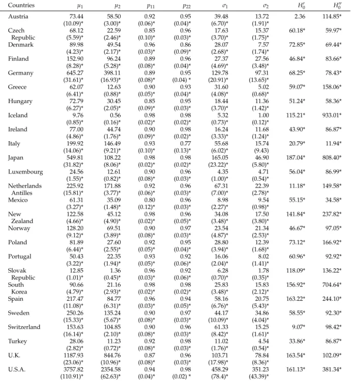
Table 1 summarizes the estimated results from the univariate MS model. There is no question that the mean of “the wave regime” (µ1)is substantially different from that of “the normal regime”
(µ2). For example, µ1 and µ2are 645 and 398, respectively, for Germany, 549 and 108 for Japan, 1187 and 844 for the U.K., and 3757 and 2345, respectively, for the U.S. They are also significantly different from zero at the conventional level. The estimated transition probabilities, p11and p22, are around 0.85 to 0.98, indicating that the duration period for remaining in a particular regime is quite long. This property is similar to the “long swing” phenomenon for the nominal exchange rate, reported by Engel and Hamilton (1990). It is not easy to evaluate the variances of the two regimes since some countries, albeit not all, have similar standard errors. Irregardless, however, the variances across remaining countries are markedly different.
We examine whether the mean of the two regimes are the same or not. Our null of the equal means (Engle and Hamilton, 1990) is:
H0′ : µ1=µ2,
3The scatter plots, the basic statistics and the results of the ADF test of the M&A activity in each of the 26 OECD
and the Wald test statistic is:
[µˆ1−µˆ2]2 c
var(µˆ1) +varc(µˆ2) −2 ccov(µˆ1, ˆµ2)
∼χ2(1).
This test statistic is free of the nuisance parameter problem, as discussed in Engel and Hamilton (1990).4 Estimated results of the null of the equal means (H0′)are reported in the second column from the right in Table 1. Except for Austria, the null hypothesis of equal means is overwhelmingly rejected. Accordingly, it is concluded that M&A activity does indeed switch between the two regimes, i.e., the wave regime and the normal regime.
We also examine whether the merger activities follow the Markov mechanism–that is, whether the number of M&A activities change for a period that cannot be completely independent of the regime that prevailed in the previous period. The null hypothesis of dependence is:
H0′′ : p11=1−p22, and µ1 6=µ2, σ12 6=σ22. Engel and Hamilton (1990) suggested using the following the Wald statistic:
[ˆp11− (1− ˆp22)]2 c
var(ˆp11) +varc(ˆp22) +2 ccov(ˆ11, ˆp22)
∼χ2(1).
The Wald test results are reported in the last column of Table 1. Because the Wald statistics are overwhelmingly significant, we reject the notion that the transition probabilities are dependent, indicating the M&A data do have a Markov mechanism. In addition, the high estimated transition probabilities suggest that a M&A wave has the “long swing” property.
We omit the graphs of the filtered and smoothed probabilities of M&A for each country be-cause of space limitations and they are available from the authors upon request. However, three interesting findings are worth noting. First, the estimated filtered and smoothed probabilities reach unity in 2000 for all OECD countries, indicating that it is a wave regime. Second, except for Mexico, New Zealand and Norway, the merger activities are rather few and far between for the remaining OECD countries in 1997. Third, though the graphs are based on a univariate study, there is a similar pattern of co-movement among the 26 OECD countries. Resende (1999) also found that sectoral patterns of M&A waves had co-movement.
We next employ the MSP model to examine the co-movement feature of M&A activities. Recall that Table 1 shows that variances across countries are substantially different. This may result in
4Many tests in switching models suffer from the nuisance problem. Readers are referred to Hansen (1992, 1996) and
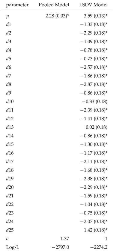
strong heteroscedasticity even though we control for the individual effect when applying the MSP model. Thus, we first adopt the weighed least-square to remove the heteroscedasticity by dividing each country’s standard deviation. Table 2 reports the estimated results from the conventional Pooled and LSDV models. All of the coefficients of the dummy variables of all countries are significant except for d13 (Netherlands Antilles). We then examine the existence of the individual effect. The null hypothesis of no individual effects is:
H0′′′ : d1=d2= · · · =d25 =0.
The log-likelihood values for the Pooled and LSDV models are−2797.0 and−2274.2, respectively, making the log-likelihood ratio (LR hereafter) 2× (−2274.2+2797.0) =1045.6 , which far exceeds the critical value of the Chi-square distraction of 37.65 at the 5% level. Therefore, the null of the no individual effect is decisively rejected, and distinct preference is given to the LSDV model over the Pooled model.
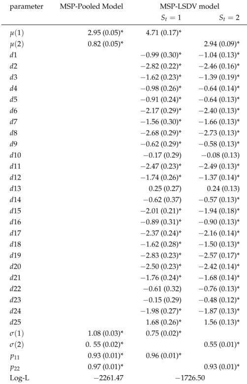
Table 3 reports the estimated results for the MSP-Pooled and MSP-LSDV models. Again, we first use the LR statistics to examine the existence of the individual effects. With the log-likelihood values for the MSP-Pooled and MSP-LSDV models being−2261.5 and −1726.5, respectively, the LR statistic is 2× (−1726.5+2261.5) =1070. Once again, as this is greater than the critical value of =67.50, the MSP-Pooled model is outright rejected; thus, the discussion below is based on the MSP-LSDV model. We also calculate the LR statistics using the conventional LSDV model as the null hypothesis (no switching) and the MSP-LSDV model as the alternative. The LR statistic is 2× (−1726.5+2274.2) = 1095.4, which also exceeds the critical value of 42.56. Thus, the MSP-LSDV is preferable to the conventional MSP-LSDV model. This is highly indicative of the fact that the sample countries follow a Markov Switching process, thus confirming the existence of common M&A waves.5
The last two columns of Table 3 report the means of the wave regime and the normal regime, which are 4.71 and 2.94, respectively, values which are significantly different from zero. The esti-mated transition probabilities for the two regimes are p11 = 0.96 and p22 = 0.93, respectively. Again, these high estimated transition probabilities indicate that M&A waves have the “long swing” property.
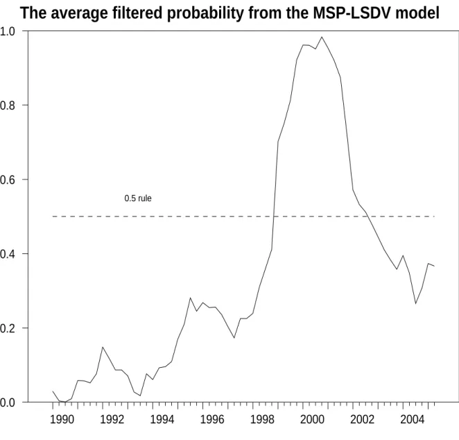
Figure 1 illustrates the average filtered probabilities from the MSP-LSDV model. According to
5Note that the LR test here suffers from the problem of the non-identified nuisance parameters. However, because
Hamilton (1989), the standard line of 0.5 is placed. As shown in the Figure, there are three small peaks: at the beginning of 1992, 1995 and 2000. The highest value falls in 2000, which coincides with the results from the univariate Markov Switching model. Also, in the 1997 sample period, the probability drop is similar to that of the univariate Markov switching model. There can be no doubt that the MS model and the MSP-LSDV model roughly show the same trend in most years, and this is especially so in 2000 and 1997. Given the weight of the evidence, we believe the MSP can really successfully describe the M&A co-movement phenomenon in our sample.
4
Concluding Remarks
This paper investigates the co-waved merger and acquisition activity in 26 OECD countries. The novelty of this paper is that we apply the conventional Markov Switching model to merger panel data (MSP here), an approach which has not been attempted in the past. Two regimes are char-acterized in the M&As data: the wave and normal regimes. Our MSP cannot reject the co-wave pattern of the sample countries. Apart from this, our MSP model has a far better fitting than the univariate MS model and the conventional linear Panel model. Also found is that M&A activity is characterized by long swing behavior. That is, the duration period for staying in a particular regime is relatively long as shown in the high estimated transition probabilities. This implies that if industries decide to merge, then the merger wave could persist for quite some time.
References
Andrestsch, D. B. (1989), The determinants of conglomerate mergers, American Economist, 33, 52–60.
Asea, P. K. and B. Bloomberg (1998), Lending cycles, Journal of Econometrics, bf 83, 89–128. Brealey, R. and S. Myers (1991), Principles of Corporate Finance, 4th ed., McGraw-Hill. New York. Dempster, A. P., N.M. Laird and D. B. Rubin (1977), Maximum likelihood from incomplete data
via the EM algorithm, Journal of The Royal Statistical Society Series, 28, 5–18.
Engel, C. and J. D. Hamilton (1990), Long swings in the dollar: Are they in the data and do markets know it? American Economic Review, 80, 687–713
Garcia, R. (1998), Asymptotic null distribution of the likelihood ratio test in Markov-switching model, International Economic Review, 39, 763–88.
Golbe, D. and White, L. (1993), Catch a wave: The time series behavior of mergers, Review of
Economics and Statistics, 75, 493–99.
Hamilton, J. D. (1989), A New Approach to the Economic Analysis of nonstationary time series and the business cycle, Econometrica, 57, 357–384.
Hamilton, J. D. (1990), Analysis of time series subject to changes in regime, Journal of Econometrics, 45, 39–70.
Hansen, B. E. (1992), The likelihood ratio test under nonstandard conditions: Testing the markov switching model of GNP, Journal of Applied Econometrics, 7, S61–S82.
Hansen, B. E. (1996), Erratum: The likelihood ratio test under nonstandard conditions: Testing the markov switching model of GNP, Journal of Applied Econometrics, 11, 195–198.
Meese, R. A. and K. Rogoff (1983), Empirical exchange rate models of the seventies: Do they fit out of sample? Journal of International Economics, 14, 3–24.
Perron, P. (1989), The great crash, the oil price shock and the unit root hypothesis, Econometrica, 57, 1361-1401.
Post, A.M. (1994), Anatomy of A Merger, London: Prentice Hall.
Resende, M. (1999), Wave behavior of mergers and acquisitions in the U.K.: A sectoral study,
Oxford Bulletin of Economics and Statistics, 61, 85–94.
Scherer F. M. and R. David (1990), Industrial Market Structure and Economic Performance, 3rd edi-tion, Boston: Houghton Mifflin,153–159
Shleifer, A. and R. Vishny (2003), Stock market driven acquisitions, Journal of Financial Economics, 70(3), 295–311.
Town, R. J. (1992), Merger waves and the structure of merger and acquisition time-series, Journal
of Applied Econometrics, 7, 83–100.
Table 1: Univariate Markov Switching model (1990:Q1–2005:Q2) Countries µ1 µ2 p11 p22 σ1 σ2 H′0 H′′0 Austria 73.44 58.50 0.92 0.95 39.48 13.72 2.36 114.85* (10.09)* (3.00)* (0.06)* (0.04)* (6.70)* (1.91)* Czech 68.12 22.59 0.85 0.96 17.63 15.37 60.18* 59.97* Republic (5.59)* (2.46)* (0.10)* (0.03)* (3.70)* (1.75)* Denmark 89.98 49.54 0.96 0.86 28.07 7.57 72.85* 69.44* (4.23)* (2.17)* (0.03)* (0.09)* (2.68)* (1.74)* Finland 152.90 96.24 0.89 0.96 27.37 27.56 46.84* 83.66* (8.28)* (5.28)* (0.08)* (0.04)* (4.69)* (3.48)* Germany 645.27 398.11 0.89 0.95 129.78 97.31 68.25* 78.43* (31.61)* (16.93)* (0.08)* (0.04) * (20.91)* (13.65)* Greece 62.07 12.63 0.90 0.93 31.60 5.02 59.07* 158.06* (6.41)* (0.88)* (0.05)* (0.04)* (4.08)* (0.68)* Hungary 72.79 30.45 0.85 0.95 18.44 11.36 51.24* 58.36* (6.27)* (2.05)* (0.09)* (0.03)* (3.70)* (1.42)* Iceland 9.76 0.56 0.98 0.98 5.32 1.00 115.21* 933.01* (0.85)* (0.16)* (0.02)* (0.02)* (0.73)* (0.12)* Ireland 77.00 44.74 0.90 0.98 16.24 11.68 43.90* 86.87* (4.86)* (1.76)* (0.09)* (0.02)* (3.33)* (1.24)* Italy 199.92 146.49 0.93 0.77 55.68 15.74 20.79* 11.94* (14.06)* (9.21)* (0.10)* (0.13)* (6.02)* (9.43) Japan 549.81 108.22 0.98 0.98 165.05 46.90 187.04* 808.40* (31.82)* (8.06)* (0.02)* (0.02)* (23.22)* (5.80)* Luxembourg 24.56 12.61 0.90 0.96 4.35 4.71 56.04* 86.99* (1.55)* (0.82)* (0.08)* (0.03)* (1.00)* (0.54)* Netherlands 225.92 171.88 0.92 0.96 67.31 22.39 11.18* 149.58* Antilles (15.81)* (3.77)* (0.06)* (0.03)* (7.00)* (2.78)* Mexico 61.31 35.09 0.80 0.96 8.98 9.54 55.15* 34.58* (3.27)* (1.48)* (0.12)* (0.03)* (2.27)* (0.98)* New 122.58 45.12 0.98 0.96 34.08 17.50 141.84* 237.82* Zealand (4.66)* (4.90)* (0.02)* (0.05)* (3.48)* (3.80)* Norway 128.20 69.51 0.90 0.97 23.54 21.34 46.67* 97.05* (9.12)* (3.89)* (0.08)* (0.03)* (4.87)* (2.53)* Poland 81.89 27.60 0.92 0.95 28.80 12.39 73.12* 166.92* (6.44)* (2.55)* (0.05)* (0.04)* (3.94)* (1.68)* Portugal 50.43 22.35 0.93 0.92 16.06 8.02 60.96* 92.92* (3.22)* (1.94)* (0.05)* (0.06)* (2.04)* (1.41)* Slovak 12.85 1.36 0.96 0.92 6.28 1.78 118.09* 136.22* Republic (1.01)* (0.45)* (0.03)* (0.06)* (0.70)* (0.35)* South 90.66 21.16 0.98 0.98 25.83 15.83 156.92* 704.64* Korea (4.79)* (2.93)* (0.02)* (0.02)* (3.48)* (2.12)* Spain 217.47 84.77 0.96 0.94 58.16 20.75 163.22* 244.10* (11.08)* (6.31)* (0.03)* (0.05)* (6.76)* (5.43)* Sweden 250.26 135.24 0.90 0.97 44.17 34.86 58.55* 92.30* (15.33)* (5.67)* (0.08)* (0.03)* (10.09)* (4.04)* Switzerland 153.63 104.85 0.90 0.96 61.33 15.25 9.07* 98.42* (16.14)* (2.10)* (0.08)* (0.03)* (8.42)* (1.61)* Turkey 28.06 11.23 0.92 0.98 11.02 4.54 33.86* 86.87* (2.82)* (0.72)* (0.08)* (0.03)* (1.76)* (0.54)* U.K. 1187.93 844.76 0.87 0.96 103.71 78.84 163.54* 102.09* (23.06)* (10.96)* (0.08)* (0.03)* (17.98)* (8.36)* U.S.A. 3757.82 2354.58 0.94 0.98 458.29 351.23 161.13* 381.34* (110.91)* (62.63)* (0.04)* (0.02) * (78.4)* (43.39)*
The numbers in parentheses are standard errors, * denotes significance at the 5% level.
Table 2: Conventional Panel model (1990:Q1–2005:Q2)
parameter Pooled Model LSDV Model
µ 2.28 (0.03)* 3.59 (0.13)* d1 −1.33 (0.18)* d2 −2.29 (0.18)* d3 −1.09 (0.18)* d4 −0.78 (0.18)* d5 −0.73 (0.18)* d6 −2.57 (0.18)* d7 −1.86 (0.18)* d8 −2.87 (0.18)* d9 −0.86 (0.18)* d10 −0.33 (0.18) d11 −2.39 (0.18)* d12 −1.41 (0.18)* d13 0.02 (0.18) d14 −0.86 (0.18)* d15 −1.30 (0.18)* d16 −1.17 (0.18)* d17 −2.11 (0.18)* d18 −1.68 (0.18)* d19 −2.38 (0.18)* d20 −2.29 (0.18)* d21 −1.59 (0.18)* d22 −1.04 (0.18)* d23 −0.75 (0.18)* d24 −2.07 (0.18)* d25 1.42 (0.18)* σ 1.37 1 Log-L −2797.0 −2274.2
Numbers in parentheses are standard errors. * denotes significance at the 5% level.
Table 3: Markov Switching Panel Model (1990:Q1–2005:Q2) parameter MSP-Pooled Model MSP-LSDV model
St=1 St=2 µ(1) 2.95 (0.05)* 4.71 (0.17)* µ(2) 0.82 (0.05)* 2.94 (0.09)* d1 −0.99 (0.30)* −1.04 (0.13)* d2 −2.82 (0.22)* −2.46 (0.16)* d3 −1.62 (0.23)* −1.39 (0.19)* d4 −0.98 (0.26)* −0.64 (0.14)* d5 −0.91 (0.24)* −0.64 (0.13)* d6 −2.17 (0.29)* −2.40 (0.13)* d7 −1.56 (0.30)* −1.66 (0.13)* d8 −2.68 (0.29)* −2.73 (0.13)* d9 −0.62 (0.29)* −0.58 (0.13)* d10 −0.17 (0.29) −0.08 (0.13) d11 −2.47 (0.23)* −2.49 (0.13)* d12 −1.74 (0.26)* −1.37 (0.14)* d13 0.25 (0.27) 0.24 (0.13) d14 −0.62 (0.37) −0.57 (0.13)* d15 −2.01 (0.21)* −1.94 (0.18)* d16 −0.89 (0.31)* −0.90 (0.13)* d17 −2.37 (0.24)* −2.16 (0.14)* d18 −1.62 (0.28)* −1.50 (0.13)* d19 −2.83 (0.23)* −2.57 (0.17)* d20 −2.50 (0.23)* −2.42 (0.14)* d21 −1.76 (0.24)* −1.68 (0.14)* d22 −0.61 (0.32) −0.76 (0.13)* d23 −0.15 (0.29) −0.48 (0.12)* d24 −1.98 (0.27)* −1.87 (0.13)* d25 1.68 (0.26)* 1.56 (0.13)* σ(1) 1.08 (0.03)* 0.75 (0.02)* σ(2) 0. 55 (0.02)* 0.55 (0.01)* p11 0.93 (0.01)* 0.96 (0.01)* p22 0.97 (0.01)* 0.93 (0.01)* Log-L −2261.47 −1726.50
Numbers in parentheses are standard errors. * denotes significance at the 5% level.