國 立 交 通 大 學
環 境 工 程 研 究 所
碩士論文
奈米微粒與次微米微粒
在氣膠微粒質量分析儀中的傳輸函數
The Transfer Function of Nanoparticles and Submicron
Particles in the Aerosol Particle Mass Analyzer
研 究 生:廖 伯 熙
指導教授:蔡 春 進 博士
奈米微粒與次微米微粒
在氣膠微粒質量分析儀中的傳輸函數
The Transfer Function of Nanoparticles and Submicron
Particles in the Aerosol Particle Mass Analyzer
研 究 生:廖伯熙 Student:Bo-Xi Liao
指導教授:蔡春進 博士 Advisor:Dr. Chuen-Jinn Tsai
國
立 交 通 大 學
環境工程研究所
碩
士 論 文
A Thesis
Submitted to Institute of Environmental Engineering College of Engineering
National Chiao Tung University in partial Fulfillment of the Requirements
for the Degree of Master
in
Environmental Engineering June 2013
Hsinchu, Taiwan, Republic of China
i
奈米微粒與次微米微粒
在氣膠微粒質量分析儀中的傳輸函數
研究生: 廖伯熙 指導教授:蔡春進 博士
國立交通大學環境工程研究所
摘 要
氣膠微粒質量分析儀(APM, Kanomax, Japan)是一部應用離心力與靜電力測量奈米微 粒與次微米微粒質量的儀器。過去的文獻指出,微粒在 APM 內部的擴散損失是造成模 擬計算值高估實驗數據(例如:質量分佈)的原因,然而至今仍未有研究能將其差異進行量 化(Lall et al., 2009, Tajima et al., 2011)。本研究利用二維數值模式研究奈米微粒與次微米 微粒在 APM 中的傳輸函數,當假設 APM 中篩選區域的流場為拋物線分佈時,發現本 模式的傳輸函數模擬結果與過去採用相同流場的文獻結果相符,但仍舊如過去文獻一樣 會高估實驗值。當本研究進一步考慮到因旋轉的篩選區域所引起的強制渦旋及採用更詳 細的計算域時,發現旋流出現在 APM 內部的流場,這些出現旋流的區域增強了奈米微 粒在 APM 儀器裡的對流擴散損失。本研究的研究結果顯著地提高了模式對 APM 傳輸 函數與反應譜的計算準確度。本研究亦根據的數值結果發展出了修正的 Ehara 模式,該 模式可更容易及準確地計算傳輸函數。利用本研究所發展出的模式,預期在未來可發展 出準確的即時奈米微粒與次微米微粒的質量分佈量測。 關鍵字: 氣膠微粒值量分析儀、APM、傳輸函數、擴散損失、旋流、模式
ii
The Transfer Function of Nanoparticles and Submicron particles in the
Aerosol Particle Mass Analyzer
Student: Bo-Xi Liao Adviser: Prof. Chuen-Jinn Tsai
Institute of Environmental Engineering
National Chiao Tung University
Abstract
The Aerosol Particle Mass Analyzer (APM, Kanomax, Japan) is one of the popular instruments to measure the mass of nanoparticles and submicron particles. In previous studies, particle diffusion loss in the APM was speculated to be the reason why simulated response functions for the APM overestimated the experimental data. But no models were available to quantify the differences (Lall et al., 2009, Tajima et al., 2011). This thesis studies the transfer function of the APM by using a 2-D numerical model for nanoparticles and submicron particles. At first, the flow field in the annular classifying region of the APM is assumed to be parabolic. It is found that the transfer functions simulated by the present model are in good agreement with previous studies which also considered the parabolic flow profile. But transfer functions are still overestimated just like previous studies. After solving detailed flow and particle concentration fields in the APM by considering the forced vortex due to the rotating classifying region as well as inlet and outlet regions in the calculation domain, recirculation flow regions are found to exist in the APM. These recirculation flow regions lead to enhanced convection-diffusion loss of nanoparticles in the APM. As a result, the present model improves the accuracy of the transfer functions and response spectra of the APM significantly. Based on the numerical results, a modified Ehara model is developed to ease the calculation of the transfer function. Using these models, it is expected that accurate real time mass distribution measurement of both nanoparticles and
iii
submicron particles can be realized in the future.
Keywords: Aerosol Particle Mass Analyzer, APM, Transfer Function, Diffusion Loss,
iv
誌 謝
十萬分地感謝指導教授蔡春進博士的指導與鼓勵,並願意給我機會在適當的壓力下 磨練自己,老師的用心指導也讓我在氣膠與環工專業領域方面獲益良多,為我的碩士論 文打下好的基礎。口試委員吳宗信教授、黃正雄教授、林文印副教授與預口試委員簡弘 民博士的悉心指教與建議,使本論文更加完整。 特別感謝學長冠宇博士無私的經驗分享與專業的支援,使本論文得以完成,學長能 駿的耐心討論也使本論文更加完整,學長俊男博士的鼓勵與私房單車路線也使我在巨大 壓力下得以放鬆,學長簡志良博士經驗與知識交流也使研究更嚴謹,學長毅弘專業軟體 技術傳授也使本論文圖表品質顯著提升,很感謝學長紹銘平時對我的鼓勵與技術上的支 援,以及學長栢森無論在畢業前後都予以熱心的幫忙,學長盧緯在我剛入學時給予的寶 貴經驗分享,以及學姐香茹、盈禎平日對我的鼓勵也讓我受益良多。也非常地感謝好同 窗國瑞的相挺、思帆的支持、瑞喬的幫忙、危涵的鼓勵、Cuc 的英語與經驗分享、葉川 的相伴,沒有你們的支持、幫忙與包容,我很幸運有這麼棒的同學;另外也要感謝實驗 室的外籍同學羅瑞格、威德、紅幸與 Aditiya 平時的外語訓練與專業知識分享,使我的 英文與報告撰寫能力得以顯著提升。助理秉才、偉恩、芳竹與佳芬平時對我的經驗分享 與幫助也讓我學到很多。學弟麒鈺、博哲與學妹慧娟的加入也使實驗室的氣氛更加活耀。 還有大學同窗家榮在我考碩班時的土地公仙草蜜以及學姐芝萍在我入學後的支援,以及 諸多朋友的相挺,使我的碩士研究之路不孤獨。教授高正忠給我的教誨與轉機也讓我受 益良多,也很感謝大學恩師教授李志源的栽培與忠告使我能有所發揮。 我也非常非常感謝守護我的健康的唐季祿醫師、江泰平醫師、楊健志醫師、曾興隆 醫師,有你們的專業醫療,我才有機會踏進交大完成論文。我也非常感謝女朋友柏安點 點滴滴的支持與包容,也給了我無比的溫暖。 最後,將本篇論文獻給我的母親素蓉、父親煌銘與姐姐庭萱,沒有你們的支持,我 不會有今天的成就,我很感謝這一切。v
Acknowledgement
I very appreciate my adviser, Prof. Chuen-Jinn Tsai, who gave me chance to study with his group and encourages me. The knowledge of aerosol science and technology that professor taught us constructs the foundation of the study. Moreover, with the suggestions given by committees Prof. Chong-Sin Gou, Prof. Cheng-Hsiung Huang, Prof. Wen-Yinn Lin, and Dr. Hung-Min Chein, the thesis becomes more complete.
I also appreciate Dr. Guan-Yu Lin’s professional supports and valued experience. Without his help, the study cannot be accomplished with such good results. In addition, Neng-Jium, who is always willing to discuss and share the experiences with me, makes the study becomes complete. Chun-Nan’s encouragements help me to challenge myself, and Yi-Hung’s professional software supports greatly improve the qualities of the figure in the thesis. Chiao-Jin’s technology supports are important to the study, and Bo-Sen, Lu-Wei, Shian-Ru, and Ying-Jen also helped me a lot. I also thank my dear classmate Guo-Ruei, Sih-Fan, Jui-Chiao, Wei Han, Cuc, and Ye-Chuan for their supports, encouragements and tolerations. I also appreciate international student Dr. Rodrigo, Virat, Hanh, Aditiya, who are willing to discuss with me about the study and English. Assistant Bing-Tsai, Wei-En, Fang-Ju, and Jia-Fen also helped me a lot. Fresh men Chi-Yu, Po-Che, and Hui-Chuan also enrich the life in laboratory. I also appreciate my college classmate Jia-Rung, and Jhih-Ping, who have helped me when I am a fresh man, and thank my friends who always support me. Prof. Cheng-Chung Kao’s suggestions also helped me a lots. Prof. Chi-Yuan Lee’s teachings and advisements also play an important role to my life of graduate student.
I specially thank Dr. Jih-Luh Tang, Dr. Tai-Ping Jiang, Dr. Jian-Zhi Yang, and Dr. Xing-Long Ceng for keeping me healthy. I also very appreciate my dear girlfriend Bo-An, who always supporting me and enriching my life.
vi
Table of Contents
摘 要 ... i Abstract ... ii 誌 謝 ... iv Acknowledgement ... v Table of Contents ... viList of Tables ... viii
List of Figures ... ix Symbols ... xi 1 Introduction ... 1 2 Literature Review ... 4 2.1 Non-Diffusion Model ... 5 Theoretical Model ... 5 2.2 Diffusion Model ... 6
Diffusion Loss of Nanoparticles ... 6
Numerical Model ... 7
2.3 Verification of the Models ... 8
3 Numerical Method ... 11
3.1 2-D Numerical Model ... 12
Governing Equation ... 12
Dimensionless Numbers for two Different APM models ... 18
3.2 Model with Classifying Region Domain and Parabolic Flow Profile ... 20
Calculation Domain ... 20
vii
Boundary Condition ... 22
Compared with Previous Studies ... 22
3.3 Model with Extended Domain and Detailed Flow Profile... 25
Calculation Domain ... 26
Flow Field ... 27
3.4 Simplified Model ... 28
Fitting Model ... 28
Modified Ehara Model ... 32
4 Results ... 37
4.1 Diffusion Loss Prediction ... 38
4.2 Recirculation Flow ... 40
4.3 APM Response Spectra ... 43
Response Spectra ... 43
Notice and Restrictions of the Models ... 49
5 Conclusion ... 50
Reference ... 52
Appendix A Some Properties of Previous Models ... 54 Appendix B The Geometry of Classifying Region of the APM Applied in Previous Studies . 56
viii
List of Tables
Table 1 The summary of the performance of previous models ... 11
Table 2 The geometry and performance of the APMs (Kanomax Inc.) ... 18
Table 3 Parameters presented in compared papers. ... 23
Table 4 The results of fitting numerical transfer function with Gaussian distribution. ... 29
Table 5 The parameters of equations which are applied to fitted the obtained and X. ... 31
Table 6 The heights of the transfer functions calculated with different flow field. ... 41
Table 7 The difference between the heights of the calculated response spectra and experimental response spectra (λc=0.22). ... 48
Table 8 The difference between the heights of the calculated response spectra and experimental response spectra (λc=0.49). ... 48
ix
List of Figures
Fig. 1. The schematic diagram of the APM (right) and its mechanism of classification (left) (KANOMAX Inc.). ... 1 Fig. 2. A typical transfer function of the APM with respective to (a) the specific mass and (b)
diameter of spherical particles. ... 3 Fig. 3. Theoretical and experimental normalized particle concentration. (Tajima et al., 2011)
... 9 Fig. 4. Scheme of the APM and the flux of particles induced in the APM. ... 12 Fig. 5. The ranges of the dimensionless numbers for APM-3600 and APM-3601 ... 19 Fig. 6. Caculation domain is the annular classifying region of the APM (dark orange area). The area enclosed by thick red lines is the rotating region. ... 21 Fig. 7. (a) The relative width and (b) the maximum height of the transfer functions for
different flow field applied to the Ehara model (Ehara et al., 1996). ... 23 Fig. 8. The transfer function of comparing our model with (a) the theoretical model
developed by Ehara et al., (1996), (b) the SDE model developed by Hagwood et al., (1995), (c) the diffusion model developed by Olfert and Collings (2005). ... 24 Fig. 9. The extended calculation domain (dark orange area) (Kanomax Inc.) ... 26 Fig. 10. Comparison between the numerical transfer function (solid lines) and the transfer
function predicted by the fitting model (dashed lines) ... 31 Fig. 11. Four particular specific masses ... 33 Fig. 12. The calculated penetration of particles passing through the still APM. ... 35 Fig. 13. The transfer functions are calculated with Ehara model (dashed black line) and
modified Ehara model (solid black line). The modified Gormley and Kennedy equation applied in modified Ehara model is dented as solid red line. ... 37 Fig. 14. The penetration of particles passing through the still APM-3600 ... 38
x
Fig. 15. The transfer functions of nanoparticles are simulated with parabolic flow field
(dashed lines) and detailed flow filed (solid lines) respectively... 40
Fig. 16. The transfer functions of submicron particles are simulated with parabolic flow field (dashed lines) and detailed flow filed (solid lines) respectively... 41
Fig. 17. The front region of the classifying region (Marked by green rectangular) ... 42
Fig. 18. The flow filed at the front region of the classifying region of the APM-3601 rotating with (a) 0 rpm, (b) 4487 rpm, (c) 11227 rpm, and (d) 13147 rpm. V5 denotes velocity (m/s). ... 42
Fig. 19. The scheme of DMA-APM measurement system ... 44
Fig. 20. The APM response spectra calculated with fitting model. (λC=0.22) ... 46
Fig. 21. The response spectra calculated with the modified Ehara model. (λC=0.22) ... 47
xi
Symbols
A Cross section area of the classifying region of the APM (m2)
B Mobility of particle (m/N.s)
Bc Mobility of center particle (m/N.s)
C(dp,c) Cunningham slip correction factor
dp Diameter of particle (nm or m)
dp,c Diameter of center particle (nm or m)
D The diffusivity or diffusion coefficient (m2/s)
Dc Diffusivity or diffusion coefficient of center particles (m2/s)
Dh Hydraulic diameter of the classifying region
E Charge of an electron (C/#)
Er Strength of electric field (N/C)
K Calibrating factor for Gormley and Kennedy equation
L Length of the classifying region of the APM (m)
M Mass of the particle (Kg)
n Number of electron on the particle (#)
Nin(S), Nout(S) Particle concentration at the APM inlet (#/m3)
Nin(dp), Nout(dp) Particle concentration at the APM outlet (#/m3)
Nin(dp,r) Number concentration of particle with diameter dp at the position r of the
inlet of the classifying region (#/m3)
Np Number concentration of particles in the APM (#/m3).
Nout(dp,r) Number concentration of particle with diameter dp at the position r of the
outlet of the classifying region (#/m3)
Nout(V) Particle concentration at the outlet of the APM operated with voltage V
xii
Np∗(r, z) Particle concentration at the position (r,z) (#/m3)
P Wet perimeter (m)
PG&𝐾 Particle penetration calculated with Gormley and Kennedy equation
P′G&𝐾 Particle penetration calculated with modified Gormley and Kennedy
equation
q Charge on the particle (C)
Q Flow rate of the flow entering APM (lpm)
r Distance from the z axis shown in Fig. 1 to the position of particle (m) r(S) Distance from the z axis shown in Fig. 1 to the position of the particle
with specific mass S that makes the particle suffer equivalent electrostatic force and centrifugal force (m)
r1 Inner radius of the classifying region (m).
r2 Outer radius of the classifying region (m)
rc The average of r2 and r1, (r2+r1)/2(m)
S Specific mass of particles (Kg/C)
Sc Specific mass of the center particle (Kg/C)
Su Source term derived the Navier-Stoke equation.
S1± Maximum and Minimum specific mass of particles which can pass
through the APM (for uniform flow field) (Kg/C)
S2± Maximum and Minimum specific mass of particles that define the shape of the transfer function (for uniform flow field) (Kg/C)
Temp. Temperature (℃)
u� Average speed of the flow passing through the classifying region of the APM (m/s).
u�⃑ Velocity of the aerosol flow passing through the APM (m/s). uc Velocity of particle flow induced by centrifugal force (m/s).
xiii
ue Velocity of particle flow induced by electric force (m/s).
ur Velocity of the flow in r direction (m/s)
uz Velocity of the flow in r direction (m/s)
uz(r) Velocity of the flow filed in the classifying region of the APM (m/s)
uθ Velocity of the flow in θ direction (m/s)
V Voltage applied on the APM (volt)
Vc Voltage of the APM operated with λc for chosen specific mass Sc or size
dp,c of particles (volt)
X Parameters of the fitting model
Zp Electrical mobility of aerosol (m2/Volt.s)
Zp,c Electric mobility of center particles (m2/Volt.s) (Eq. (20))
β1 Dimensionless number
β2 Dimensionless number
β3 Dimensionless number
δ Half distance of the gap, which is described by (r2-r1)/2 (m)
ζ Normalized coordinate in z direction, ζ = z
L
η Dimensionless number
ηc Dimensionless number of the center particle
λMFP Mean free path of carrier gas (m)
λ Classification performance parameter (dimensionless number)
λc Classification performance parameter of the center particle
(dimensionless number)
Viscosity of the fluid (N.s/m2)
ρ(S) Position of particle with specific mass S in normalized r coordinate, ρ(S) = [r(S)−rc]
xiv
ρgas Density of carrier gas (Kg/m3)
The standard deviation of the fitting model (volt)
τ Relaxation time of particle (s)
τc Relaxation time of the center particle (S)
ω Rotation speed of the APM (rad/s)
ΩAPM(dp) APM transfer function of particles with diameter dp
ΩAPM�dp, ωλc, V� Transfer function of particles with diameter dp passing through the APM
operated with rotation speed ωλc and V
ΩAPM(S) APM transfer function of particles with specific mass S
ΩAPM(S, ωλc, V) Transfer function of particles with specific mass S passing through the
APM operated with rotation speed ωλc and V
Ω𝐴𝑃𝑀′ (𝑠) The APM transfer calculated with the modified Ehara model
ΩDMA�dp, VDMA� Transfer function of particles with diameter dp passing through the DMA
1
1 Introduction
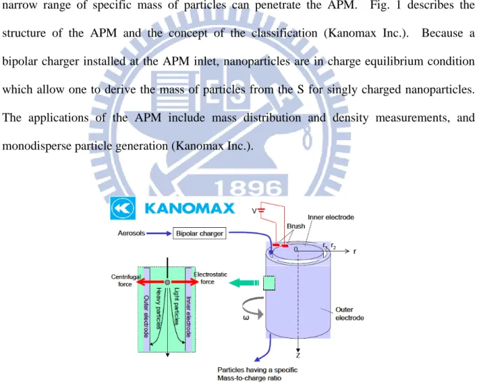
The Aerosol Particle Mass Analyzer (APM) classifies particles based on their mass to charge ratios or specific masses, denoted as S (Kg/C), by using centrifugal and electrostatic forces (Ehara et al., 1995, Ehara et al., 1996). The direction of the forces is reverse to each other. When the centrifugal force is greater than electrostatic force, the particle will be removed by the centrifugal force. Similarly, when the electrostatic force is greater than the centrifugal force, the particle will be removed by the electrostatic force. Therefore, only narrow range of specific mass of particles can penetrate the APM. Fig. 1 describes the structure of the APM and the concept of the classification (Kanomax Inc.). Because a bipolar charger installed at the APM inlet, nanoparticles are in charge equilibrium condition which allow one to derive the mass of particles from the S for singly charged nanoparticles. The applications of the APM include mass distribution and density measurements, and monodisperse particle generation (Kanomax Inc.).
Fig. 1. The schematic diagram of the APM (right) and its mechanism of classification (left) (KANOMAX Inc.).
2
electrostatic force are in balance in the APM as well as the specific mass:
m × ω2× r = n×e×V r×ln(r2r1) (1) S = m n×e= m q = V ω2r2×ln(r2 r1) (2)
m: Mass of the particle (Kg)
ω: Rotation speed of the APM (rad/s)
r: Distance from the z axis shown in Fig. 1 to the position of particle (m) n: Number of electron on the particle (#)
e: Charge of an electron (C/#)
V: Voltage applied on the APM (volt)
r1: Inner radius of the classifying region (m).
r2: Outer radius of the classifying region (m)
q: Charge on the particle (C)
The transfer function is the ratio of the particle concentration at the outlet to that at the inlet of the APM. With a specific rotation speed, voltage, and flow rate, each specific mass of particles has a particular transfer function. In addition, if the particle is spherical, the specific mass can be converted to the size of particle with a known density. Eq. (3) describes the transfer function based on the diameter of the particle (denoted as ΩAPM(dp)) or the
specific mass of the particle (denoted as ΩAPM(S)).
ΩAPM(S) =NNoutin(S)(S) or ΩAPM�dp� =NNoutin�d�dpp�� (3)
3
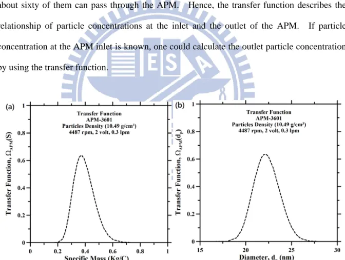
concentration at the APM inlet. Fig. 2 is the example of the transfer function. When the rotation speed and the voltage of the APM-3601 are 4487 rpm and 2 volt respectively, only particles with specific mass ranges from 0.2 Kg/C to 0.7 Kg/C can pass through the APM as shown in Fig. 2(a). If the particles are spherical, the specific masses can be converted to the diameters that the particles with diameter ranging between 18 nm to 28 nm can pass through the APM. In Fig. 2, singly charged 22 nm (or 0.37 Kg/C) particles have the maximum transfer function, which is about 0.64. In other words, if there are one hundred 22 nm particles entering the APM with homogeneous concentration at the inlet of the APM, only about sixty of them can pass through the APM. Hence, the transfer function describes the relationship of particle concentrations at the inlet and the outlet of the APM. If particle concentration at the APM inlet is known, one could calculate the outlet particle concentration by using the transfer function.
Fig. 2. A typical transfer function of the APM with respective to (a) the specific mass and (b) diameter of spherical particles.
Because the transfer function builds up the relationship between the particles concentrations at the outlet and the inlet of the APM, the calculation of transfer function is
4
important. Several models have been developed to calculate the transfer function in the literature (Ehara et al., 1995, Hagwood et al., 1995, Ehara et al., 1996, Olfert and Collings 2005). For submicron particles, some models have been verified with experimental data (Ehara et al., 1996, Tajima et al., 2011). For nanoparticles, however, no model has agreed well with the experimental data. Most of the theoretical or numerical models overestimated the peak values of the transfer functions as compared to the experimental data (Lall et al., 2009, Tajima et al., 2011). Previous studies concluded that the differences between the theoretical results and experimental results were due to the diffusion loss caused by Brownian motion (Lall et al., 2009, Tajima et al., 2011). Even when the particle diffusion loss was considered, the models still overestimated the transfer function as compared to experimental data (Olfert et al., 2006, Lall et al., 2009). Hence, the purpose of the study is to improve the accuracy of the transfer function of nanoparticles in the APM.
2 Literature Review
Several models have been developed in the past to calculate the transfer function. Ehara et al., (1995) and Ehara et al., (1996) pioneered the development of the theoretical model for the transfer function based on the trajectories of the particles passing through the APM (Lagrangian approach). Hagwood et al., (1995) presented two numerical models to simulate the transfer function in consideration of effects of the diffusion loss. Based on the convection-diffusion equation, Olfert and Collings (2005) developed the diffusion model of the transfer function. In addition, some studies compared the models with experimental data. Ehara et al., (1996) verified their model with experimental submicron particle data. Lall et al., (2009) applied one of the numerical models developed by Hagwood et al., (1995) to calculate the transfer function, and Tajima et al., (2011) compared APM response spectra simulated by the theoretical model with experimental ones. The methods and the results of
5
the comparison are described in the following sections.
2.1 Non-Diffusion Model
Theoretical Model
Based on the trajectories of particles passing through the classifying region of the APM, Ehara et al., (1996) developed the original theory (theoretical model) to calculate the transfer function of the APM without considering the Brownian motion of particle. The uniform flow and parabolic flow were applied in the theoretical model respectively. Appendix A contains the details of the assumptions applied in the model.
Ehara et al., (1996) found a dimensionless number λc for the APM, which is the
dimensionless number of the transfer function for the center particles that achieve force balance of centrifugal force and electrostatic force at the central position (denoted as rc, which
is equal to the average of the r1 and r2) between the inner and the outer of the annular
cylinders (classifying region). It can be described by Eq. (4) (Ehara et al., 1996). The center particle has the maximum transfer function (roughly). For example, the center particle in Fig. 2 is the particle which has the maximum transfer function. The specific mass and the diameter of the center particle are denoted as dp,c and Sc respectively.
λc = 2τcω2L/u� (4)
τc: Relaxation time of the center particle (S)
L: Length of the classifying region of the APM (m)
u�: Average speed of the flow passing through the classifying region of the APM (m/s).
λc describes the peak height (maximum transfer function) and the resolution (relative
6
(Tajima et al, 2011). The lower and narrower transfer function occurs with greater value of λc, while the higher and wider transfer function occurs with lower value of λc. It should be
noted that if the λc of the different transfer functions were similar, the height and the shape of
those transfer functions were also similar despite differences of rotation speed, voltage or flow rate. Ehara et al., (1996) defined the phenomenon as the similarity rule. Moreover, if the value of λc was sufficiently small (ex: less than 0.3), the assumption of the differences
between the model in the uniform flow field and the parabolic flow field became insignificant (ex: Maximum height difference can be less than about 4% in transfer function). These features of the small λc indicated that the transfer function can be solved with analytical
solution; therefore, the small λc significantly reduced the complexity of the calculation.
Ehara et al., (1996) also verified the model with experimental data of monodisperse 309nm Polystyrene Latex (PSL) (Ehara et al., 1996). In summary, Ehara et al., (1996) described the relationship among the centrifugal force, the electrostatic force and the transfer function through the theoretical model.
2.2 Diffusion Model
Diffusion Loss of Nanoparticles
Nanoparicles have significant Brownian motion compared with submicron particles. The loss of nanoparticles in APM is enhanced due to the Brownian motion. The phenomenon was verified with the numerical models (Hagwood et al., 1995, Olfert and Collings 2005) and the experimental data (Lall et al., 2009 and Tajima et al., 2011). For example, Hagwood et al., (1995) found that the peak of the transfer function of 20nm particles was decreased from about 86% to 20% after considering the diffusion loss of the particles. Tajima et al., (2011) found that results simulated by the model without considering Brownian motion of particles significantly overestimated penetration of 30 nm monodisperse PSL (more than 20% on normalized particle concentration). In addition, the degree of overestimation
7
became insignificant for submicron particles (Fig. 3). The different levels of overestimation showed the effects of the Brownian motion. In sum, the Brownian motion of nanoparticles indeed has great impact on the transfer function.
Numerical Model
The theoretical model developed by Ehara et al., (1996) was accurate for submicron particles, but it overestimated the transfer function for nanoparticles due to the assumption neglecting the Brownian motion. Some numerical methods were developed to calculate the transfer function with considering the Brownian motion of particles (Hagwood et al., 1995, Olfert and Collings 2005).
Hagwood et al., (1995) developed two numerical methods, the Stochastic Differential Equation (SDE) and the Monte Carlo method (MC), to simulate the transfer function in consideration of the Brownian motion. The former calculated the transfer function based on the probability of particles passing through the APM, while the latter applied the Gaussian random variables to describe the Brownian motion. Appendix A contains some important assumptions applied to the models. The results calculated by these models showed the significant effects of the Brownian motion of nanoparticles on the transfer function.
Another numerical model was developed by Olfert and Collings (2005), which was based on the convection-diffusion equation. The study also found another dimensionless number η as described in Eq. (4). The η took the diffusivity of particles in to consideration. The effects of diffusion become important when |ηc| of the APM applied in the study was
approximately less than 10 (Olfert and Collings 2005, Olfert et al., 2006).
ηc = 2δ
2τcω2
8
: Half distance of the gap, which is described by (r2-r1)/2 (m)
Dc: Diffusivity or diffusion coefficient of center particles (m2/s)
2.3 Verification of the Models
Up to now, several models were developed. Some of the models have been compared with experimental data (Ehara et al., 1996, Olfert et al., 2006, Lall et al., 2009, Tajima et al., 2011); however, no model has accurately agreed with experimental data for nanoparticles even if the effects of Brownian motion were considered in the model.
Nout(V) = ∫ Nin(S)ΩAPM(S, V)dS (6)
Ehara et al., (1996) calculated the number concentration of monodisperse particles passing through the APM (Eq. (6)). In Eq. (6), the particle concentration at the APM outlet, denoted as Nout(V), is the function of voltage. The particle concentration at the APM inlet
was considered the function of the specific mass (denoted as Nin(S)) which was assumed to be
proportional to the function, and the transfer function of the APM was denoted as the function of the specific mass and voltage (denoted as ΩAPM(S,V)). The rotation speed of the
APM was fixed, while the voltage of the APM was shifted to scan the specific mass distribution of the particles. The theoretical relative particle concentration, which is the ratio of the total particle concentration at the APM outlet to that at the APM inlet, was calculated with different voltage and compared with the experimental one. Good agreement of the comparisons between the experimental data (monodisperse 309 nm PSL) and the simulated results showed the validity of the theoretical model.
Since the theoretical model developed by Ehara et al., (1996) neglected the Brownian motion of particles, the model is not suitable to nanoparticles. Tajima et al., (2011) applied
9
the model disregarding the Brownian motion of particles to simulate the APM response spectra which is same as the relative particle concentration calculated in Ehara et al., (1996). The flow field of the model was assumed to be parabolic. Different to Ehara et al., (1996), Tajima et al., (2011) considered the size distribution of monodisperse PSL at the APM inlet more carefully as described in Eq. (7). The size distribution of the particles at the inlet of Differential Mobility Analyzer (DMA) were considered the Gaussian distribution (denoted as N0(dp)) based on the mean and standard deviation of size of size standard PSL. Moreover,
the particles classified by the DMA (Nin(dp)) is considered the product of the N0(dp) and the
transfer function of the DMA (denoted as ΩDMA). VDMA is the voltage applied to the DMA.
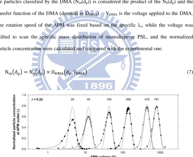
The rotation speed of the APM was fixed based on the specific λc, while the voltage was
shifted to scan the specific mass distribution of monodisperse PSL, and the normalized particle concentration were calculated and compared with the experimental one.
Nin�dp� = N0�dp� × ΩDMA�dp, VDMA� (7)
Fig. 3. Theoretical and experimental normalized particle concentration. (Tajima et al., 2011)
Fig. 3 showed the results of comparisons presented in Tajima et al., (2011). The number on each curve was the size of the monodisperse PSL. The thick grey lines were the simulated results, and the thin black lines fitted the experimental data (points) with the least
10
square fitting method. Differences between the simulated results and experimental data became significant for PSL less than 100 nm. Tajima et al., (2011) concluded that the differences (overestimations) were caused by diffusion loss.
Lall et al., (2009) applied the MC method (Hagwood et al., 1995) to calculate the APM transfer function with the assumption of the parabolic flow field, and they also calculated the particle concentration at APM outlet with the manner similar to the manner did in Tajima et al., (2011) as described in Eq. (6) and (7). Different from Tajima et al., (2011), Lall et al., (2009) considered the N0 as the constant function and applied the triangular function to the
transfer function of the DMA. Comparing to experimental data, Lall et al., (2009) found the simulated results overestimated the penetration for nanoparticles (60 nm, 100 nm PSL) and submicron particles (300 nm PSL). Lall et al., (2009) concluded that was due to diffusion losses and transport losses.
Olfert et al., (2006) verified the model presented in Olfert and Collings (2005). Instead of the APM, the major objective of the study for Olfert and Collings (2005) is the Couette Centrifugal Particles Mass Analyzer (CPMA). Because the only difference between two instruments is the rotation speeds of the inner and outer cylinders, while the cylinders of the APM have the same rotation speed, the CPMA is very similar to the APM. The different rotation speed of cylinders of the CPMA was applied in order to achieve the stabler state of the classification (decrease the loss of particles during the classification). Since the APM is very similar to the CPMA, the diffusion model developed by Olfert and Collings (2005) not only available to the CPMA but also available to the APM. Olfert et al., (2006) compared the model of the CPMA with experimental data. The assumption of parabolic flow field was made in the model, and of assuming that particles at the APM inlet are strict monodisperse (particles are in same size). For 50 nm PSL, the diffusion model significantly overestimated the transfer function compared to the experimental data. Olfert et al., (2006) concluded that the overestimation was due to the particle diffusion. Because the model of the CPMA is
11
very similar to the model of the APM, we consider that the result concluded for the CPMA in Olfert et al., (2006) would also be available to the APM.
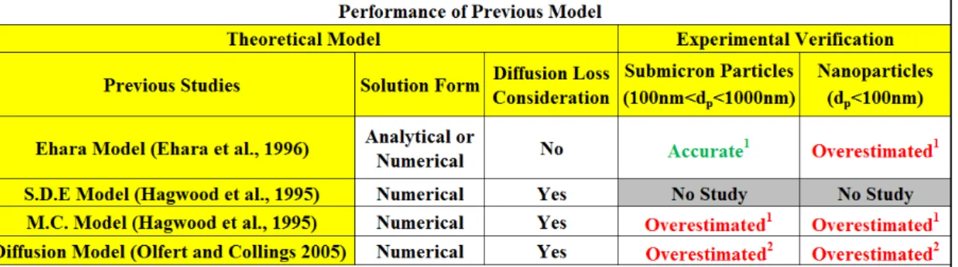
In sum, for submicron particles, some models have been verified by the experimental data (Ehara et al., 1996, Tajima et al., 2011). For nanoparticles, however, no model has agreed well with experimental data. Table 1 summarizes the performance of previous transfer function models.
Table 1 The summary of the performance of previous models
3 Numerical Method
A 2-D numerical model developed by our laboratory is applied to simulate the transfer function of the APM. The preliminary verification of the model is conducted with comparing the simulated transfer function with ones done by previous models with simple calculation domain (the classifying region of the APM) and assumption of parabolic flow field. After the preliminary verification, the model is further improved by extending calculation domain from classifying region to whole region in the APM and by considering detailed flow field based on the Navier-Stokes equations. The improved model is used to compare with the experimental data shown in Tajima et al., (2011) as the advanced verification.
12
3.1 2-D Numerical Model
Governing Equation
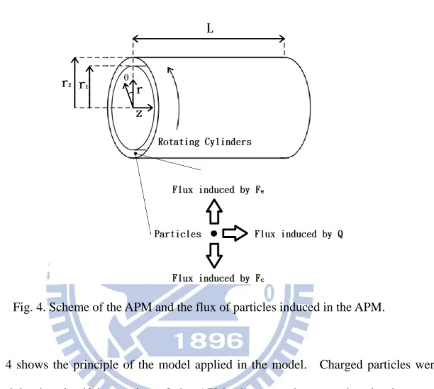
Fig. 4. Scheme of the APM and the flux of particles induced in the APM.
Fig. 4 shows the principle of the model applied in the model. Charged particles were introduced in the classifying region of the APM (the space between the closely-spaced annular cylinders). Particles passing through the region are classified by the centrifugal force Fc and electrostatic force Fe. In Fig. 4, L is the length of the APM. Three directions
of flux in the classifying region are considered. First one is the flux induced by the carrier gas. Particles move with the direction of flow in the APM. Second one is for the particles of which Fe is greater than Fc, the flux toward the inner cylinders is induced. Third one is for
particles of which Fe is smaller than Fc, the flux flowing toward the outer cylinders is induced.
The flux describe the particles which are classified by the APM.
The governing equation applied in the model is based on the convection-diffusion equation. The general equation of the convection-diffusion equation is
13
∂Np
∂t = ∇ ∙ �D∇Np� − ∇ ∙ �u�⃑Np�. (8)
Np: Number concentration of particles in the APM (#/m3).
u�⃑: Velocity of the aerosol flow passing through the APM (m/s).
It is considered that there is no source, sink or chemical reaction in the APM classifying region. The study considers that the flow in the APM is isothermal and steady. Since the Mach number of the flow is much less than 0.5 (ex: 0.0046 for the APM-3601 or 0.015 for the APM-3600), the carrier gas (ex: air) is considered as incompressible fluid. In addition, the classification of the APM is assumed to be steady (∂Np
∂t=0). Because centrifugal force and electrostatic force do not change in θ direction, the particle motion in θ direction and the flow field in θ direction are neglected in the model (uθ=0). Finally, the governing equation of 2-D model for the transfer function is
∂�ur+(uc−ue)Np�
∂r + ∂�uzNp� ∂z = D � 1 r ∂ ∂r�r ∂Np ∂r � + ∂2Np ∂z2 �. (9)
ur: Velocity of flow in r direction (m/s)
uz: Velocity of flow in z direction (m/s)
uc: Velocity of particle flow induced by centrifugal force (m/s).
ue: Velocity of particle flow induced by electric force (m/s).
r: Distance between the aerosol and the axis of the APM (m).
Eq. 9 is further rewritten with the detailed description of ue and uc, as described in Eq. (10)
14 uc = τrω2 = mBrω2 (10) ue = ZpEr(r) = Zpr lnVr2 r1 (11) ∂��τrω2−ZpEr�Np� ∂r + ∂�urNp� ∂r + ∂�uzNp� ∂z = D � 1 r ∂ ∂r�r ∂Np ∂r� + ∂2Np ∂z2 � (12)
τ: Relaxation time of particle (s) B: Mobility of particle (m/N.s) Er: Strength of electric field (N/C)
Zp: Electrical mobility of aerosol (m2/Volt.s)
Several dimensionless parameters are applied to obtain the dimensionless form of Eq. (12). These parameters are listed in Eq. (13) to Eq. (20) respectively.
Np∗ =NNinp (13) uz∗ =uu�z (14) ur∗ = uu�r (15) r∗ = r 4δ (16) z∗ = z 4δ (17) Zp∗ =ZZp,cp (18) τ∗ = τ τc (19) D∗ = D Dc (20)
15
Nin: Particle concentration at the APM inlet (#/m3)
Zp,c: Electric mobility of center particles (m2/Volt.s) (Eq. (21))
Bc: Mobility of center particle (m/N.s)
dp,c: Diameter of center particle (m) (Eq. (22))
C(dp,c): Cunningham slip correction factor (Eq. (23))
Zp,c = qBc = ne3πµdC�dp,cp,c�κ (21) dp,c= �πρ 6Vne gasrc2ω2ln�r2r1�� 1 3 (22) C�dp� = 1 + �2λdMFPp � �1.142 + 0.558exp �−0.999d2λMFPp�� (23)
ρgas: Density of carrier gas (Kg/m3)
λMFP: Mean free path of carrier gas (m).
The 4δ shown in the denominator of Eq. (16) and (17) is the characteristic length of the APM. In the study, the hydraulic diameter of the classifying region (Dh) is considered the
characteristic length (Eq. 24). In Eq. (24), A is the cross section area of the classifying region of the APM (m2), and P is the wet perimeter, the sum of the circumferences of inner and outer radius of the classifying space (m).
Dh = 4AP =4π�r2
2−r 1 2�
2π(r2+r1) = 2(r2− r1) = 4δ (24)
16 ∂��τcτ∗ω2r∗4δ��N0Np∗�� 4δ ∂r∗ − ∂��Zp∗Zp,c4δr∗K ��N0Np∗�� 4δ ∂r∗ + ∂�(u�ur∗)�N0Np∗�� 4δ ∂r∗ + ∂�(u�uz∗)�N0Np∗�� 4δ ∂z∗ = DcD∗��4δr1∗� ∂ 4δ ∂r∗�4δr∗ N 0∂Np∗ 4δ ∂r∗� + N0 (4δ)2 ∂2Np∗ ∂z∗2�. (25)
Eq. (25) can be further rewritten to be Eq. (26).
τcω2 ∂�τ ∗(r∗)�Np∗�� ∂r∗ − Zp,cK (4δ)2 ∂�Zp∗ Np ∗ r∗� ∂r∗ +4δu� ∂�ur∗Np∗� ∂r∗ +4δu� ∂�uz∗Np∗� ∂z∗ = Dc (4δ)2�D∗� 1 r∗� ∂ ∂r∗�r∗ ∂Np ∗ ∂r∗� + D∗ ∂ 2Np∗ ∂z∗2� (26) where K is V
ln�r2r1�. After dividing Eq. (26) by u� 4δ, we can obtain 4δτcω2 u� ∂�τ∗(r∗)�Np∗�� ∂r∗ − Zp,cK 4δu� ∂�Zp∗ Np ∗ r∗� ∂r∗ + ∂�ur∗Np∗� ∂r∗ + ∂�uz∗Np∗� ∂z∗ = Dc 4δu��D∗� 1 r∗� ∂ ∂r∗�r∗ ∂Np ∗ ∂r∗� + D∗ ∂ 2N p ∗ ∂z∗2�. (27)
Three dimensionless numbers are found from Eq. (27) as described in Eq. (28)~(30).
β1 = 4δτcω 2 u� (28) β2 =4δu� ln�Zp,cVr2 r1� (29) β3 =4δu�Dc =Pe1 (30)
The β1 includes the rotation speed of the APM, the average velocity of the carrier gas, and
the relaxation time of the center particle, which is almost same as the dimensionless number λ found by Ehara et al., (1996) (Eq. (4)). The β2 considers the electric mobility of the center
17
particle, the strength of the electric field, and the average velocity of the carrier gas. β1 and
β2 are dependent to each other through the force balance of Fc and Fe of the center particle.
The β3 includes the diffusivity of the center particle. It is considered the reciprocal Peclet
number (denoted as Pe). Greater value of β3 represents the stronger effects of the Brownian
motion. Furthermore, it is found that the ratio of β1 to β3 is just equal to eight times of the
dimensionless number η (Eq. (4)), which is described in Eq. 31. Since the β1 and β1/β3 are
similar to the λcand η respectively, the properties of λc and η should be also applicable to the
β1 and β1/β3. For example, the similarity rule found by Ehara et al., (1996) described that
when the λc of the transfer function were similar, the height and shape of the transfer
functions were similar too. The rule should be available on the β1 too. Another example is
that Olfert et al., (2006) mentioned that the effects of the diffusion are important when the absolute value of ηc is less than 10 or the absolute value of β1/β3 is less than 80 for the
simulated APM. In sum, three dimensionless numbers are derived from governing equation, and the dimensionless numbers can cover ones presented in previous studies.
β1 β3 = (4δ)2τ cω2 Dc = 8 × � 2δ2τcω2 Dc � = 8 ηc (31)
In sum, the governing equation has been developed based on the convection-diffusion equation. The governing equation will be applied to study the transfer function of nanoparticle and submicron particle of the APM. Moreover, three dimensionless numbers (β1, β2 and β3) are found. The β1 is related to the rotation speed, the β2 is related to the
voltage, and the β3 is related to the diffusivity of the particles. The obtained dimensionless
numbers can be similar to the ones presented in previous studies (ex: λc, ηc); hence, the
characteristics of the λc and ηc should be also available to our dimensionless numbers β1 and
18
Dimensionless Numbers for two Different APM models
To compare the performance between different APMs (Model 3600, Model 3601, Kanomax Japan Inc.), dimensionless numbers β1, β2 and β3 are applied to characterized their
performances. The geometry and the performance of the APMs are listed in table 2. The shape of particle is considered spherical; hence, the mass of particle can be easily converted to size with known particle density (ex: 1.05 g/cm3).
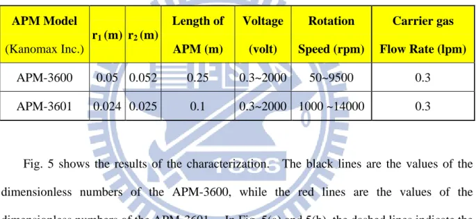
Table 2 The geometry and performance of the APMs (Kanomax Inc.)
APM Model (Kanomax Inc.) r1 (m) r2 (m) Length of APM (m) Voltage (volt) Rotation Speed (rpm) Carrier gas Flow Rate (lpm) APM-3600 0.05 0.052 0.25 0.3~2000 50~9500 0.3 APM-3601 0.024 0.025 0.1 0.3~2000 1000 ~14000 0.3
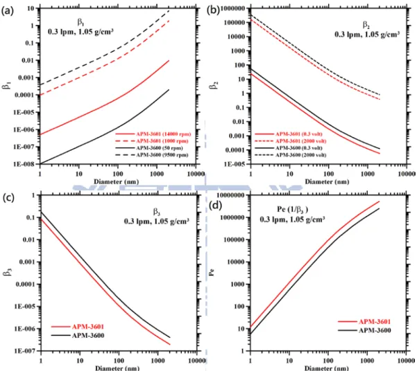
Fig. 5 shows the results of the characterization. The black lines are the values of the dimensionless numbers of the APM-3600, while the red lines are the values of the dimensionless numbers of the APM-3601. In Fig. 5(a) and 5(b), the dashed lines indicate the maximum values of the dimensionless numbers for each size of particles, and the solid lines indicate the minimum values of the dimensionless numbers.
In Fig. 5(a), the range of the β1 of the APM-3600 is wider than that of the APM-3601.
The available maximum rotation speed of the APM-3601 (14000 rpm) is higher than that of the APM-3600 (9500 rpm), yet the APM3600 can perform with wider range of the β1 than the
APM-3600 due to different size and geometry of the classifying regions. For example, when the rotation speed are the same, the radius of classifying region of the APM-3600 is longer than that of the APM-3601, it makes the APM-3600 has stronger centrifugal force compared
19
to the APM-3601. Moreover, when the APMs operated with same flow rate (0.3 lpm), the slower average velocity u� of carrier gas makes the APM-3600 has larger β1 compared to the
APM-3600.
Fig. 5. The ranges of the dimensionless numbers for APM-3600 and APM-3601
In Fig. 5(b), although the available range of voltage of both APMs is the same, the β2 of
the APM-3600 can be higher than that of the APM-3601. We conclude that it is due to slower u� of the APM-3600 compared to that of the APM-3601 when the flow rates of both APMs are the same. Hence, it is concluded that the APM-3600 can perform with the higher β2 compared with the APM-3601. Fig. 5(c) and 5(d) show the relationship between the size
20
APM-3600. It is because that the gap between the outer and inner radius of classification space of the APM-3601 is narrower than that of the APM-3600. The narrower gap makes the flow velocity of the APM-3601 higher than of the APM-3600; hence, the retention time (diffusion time) of particles passing through the APM-3601 is decreased.
In sum, the APM-3600 can operate with wilder range of the β1 and higher β2 compared to
the APM-3601, while the APM-3601 is more suitable to operate with smaller nanoparticles (less diffusion loss) compared to the APM-3600.
3.2 Model with Classifying Region Domain and Parabolic Flow Profile
In this section, the governing equation presented in chapter 3.1 is applied to build up the model. The calculation domain of the model is the classifying region of the APM and parabolic flow field is applied. The transfer functions simulated by the model are compared with ones simulated with previous models. The comparison is considered as the preliminary verification of our model. Based on the good agreements of the comparison, the model presented in the section is considered the representative of the previous models.
Calculation Domain
In Fig. 6, the dark orange area is the classifying region, which is the space between the inner and outer closely-spaced annular cylinders. Several studies considered the classifying region the calculation domain of their models (Hagwood et al., 1995, Ehara et al., 1996, Olfert and Collings 2005). To verify our model, the calculation domain of our model is defined to be the classifying region as previous studies did.
21
Fig. 6. Caculation domain is the annular classifying region of the APM (dark orange area). The area enclosed by thick red lines is the rotating region.
Flow Field
Because previous studies usually made the assumption of laminar parabolic flow field for their models (Hagwood et al., 1995, Ehara et al., 1996, Olfert and Collings 2005), we apply the same assumption of the flow field for the model. Eq. (32) is applied to describe the parabolic flow field in the classifying region of the APM.
u = uz(r) =32u� �1 − �rr−rc
2−r1�
2
� (32)
rc: The average of r2 and r1 (m), (r2+r1)/2
Eq. (33) describes the transfer function, ΩAPM, for particles with diameter dp. In eq. (33),
the number concentration of the particles at the APM inlet Nin(dp , r) is considered
homogeneous, while the number concentration of the particles at the APM outlet Nout(dp , r) is
solved numerically by the SIMPLER algorithm (Semi-Implicit Method for Pressure-Linked Equations) (Patankar 1980, Lin et al., 2010).
22 ΩAPM(dp) =2π ∫ Nout �dp,r�uz(r)dr r2 r1 2π ∫ Nr1r2 in�dp,r�uz(r)dr (33) Boundary Condition
Eq. (34) and (35) describe the boundary conditions of the model. Np∗(r, z) is the normalized particle concentration, the ratio of particle concentration at the outlet to the inlet of the APM classifying region, at the position (r,z). Np∗(r, 0), the normalized particle concentration at the inlet of classifying region, is considered as 1. In addition, because particle contacting the walls in the classifying region is removed, particle concentration at the walls is considered zero (removed by the APM).
Np∗(r, 0) = 1 for r1<r<r2 (34)
Np∗(r2, z) = Np∗(r1, z) = 0 (35)
Compared with Previous Studies
The transfer functions simulated with the model presented in this section are compared with ones simulated with three previous models respectively, which are the theoretical model developed by Ehara et al., (1996), the numerical models presented in Hagwood et al., (1995) and the diffusion model developed by Olfert and Collings (2005). To simplify the calculation, the particle is assumed spherical. The result of the comparisons is considered as the preliminary verification of the model.
For the comparisons of our model and the theoretical model (Ehara et al., 1996) and the numerical models (Hagwood et al., 1995), the parameters of the models are set to be same as the ones set in Hagwood et al., (1995) (table 3). For the comparison of our model and the diffusion model developed by Olfert and Collings (2005), the parameters of the models are set to be same as the ones used in Olfert and Collings (2005) (table 3). Because pressure and
23
temperature applied in some previous studies were unknown, we assumed the atmospheric pressure and 25 ℃ for these parameters.
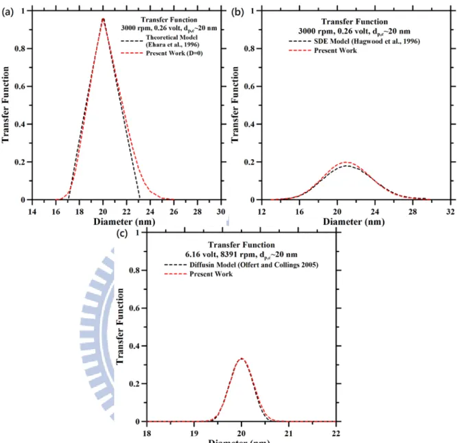
Table 3 Parameters presented in compared papers.
References r1 (m) r2 (m) L (m) Pressure (atm) Temp. (。C) Q (lpm) ρaerosol (Kg/m3) Hagwood et al., (1995) 0.1 0.101 0.2 (assumed 1) (assumed 25) 0.5 1000
Olfert and Collings (2005) 0.1 0.103 0.2 (assumed 1) 22 0.5 1000
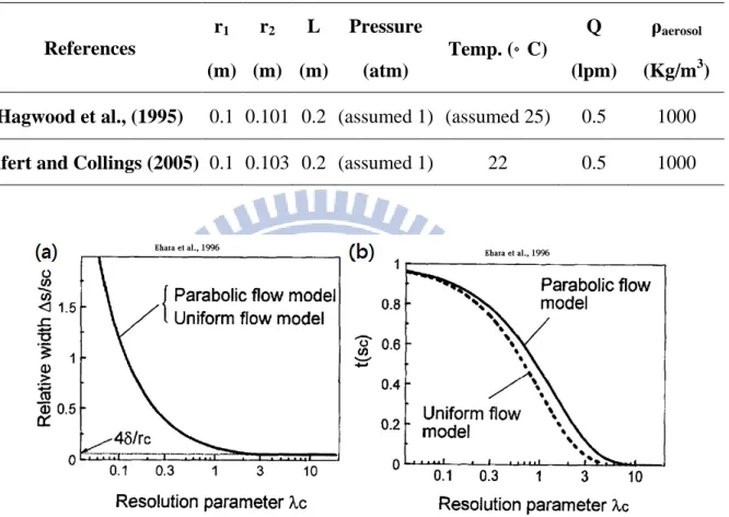
Fig. 7. (a) The relative width and (b) the maximum height of the transfer functions for different flow field applied to the Ehara model (Ehara et al., 1996).
It should be noted that Ehara et al., (1996) found that if the value of the λc is small (less
than about 0.5), there is no significant difference between the transfer functions simulated by the Ehara model with uniform flow field and parabolic flow field (Fig. 7). The λc of the
transfer function applied in the comparison of our model and Ehara model is about 0.044, which is much lower than the 0.5. Moreover, applying the uniform flow field makes the transfer function available to be solved as exact solution. Therefore, to simplify the calculation, we applied the assumption of the uniform flow field to the Ehara model.
24
Fig. 8. The transfer function of comparing our model with (a) the theoretical model developed by Ehara et al., (1996), (b) the SDE model developed by Hagwood et al., (1995), (c) the diffusion model developed by Olfert and Collings (2005).
Fig. 8 shows the result of the comparisons. In Fig. 8(a), the dashed black line is obtained with our model, while the dashed red line is obtained with the theoretical model developed by Ehara et al., (1996). Since Ehara model neglected the Brownian motion, we zero the diffusivity of our model for making the comparison (D=0). The result showed good agreement between two models. In Fig. 8(b), the transfer function obtained with our model
25
(dashed red line) agrees very well with one simulated with the SDE model (dashed black line). The slight difference would be due to different principles or governing equations of the models. The SDE model is based on the escaped probability of particles whereas our model is based on the convection-diffusion equation. Fig. 8(c) shows the comparison of our model and the diffusion model developed by Olfert and Collings (2005). The transfer function simulated with our model is denoted as dashed red line, while the one simulated with the diffusion model is denoted as dashed black line.
In sum, the transfer functions simulated by our model agreed well with several models which were presented in previous studies. The good agreement is considered as the preliminary verification of the model. The verified model is considered as the representative of the previous models, whose calculation domain is the classifying region of the APM and the flow field is assumed parabolic.
3.3 Model with Extended Domain and Detailed Flow Profile
Although the model with classifying region domain and parabolic flow profile agrees very well with several previous studies, none of the previous models has agreed well with experimental data of nanoparticles even the model considered the diffusivity of particles. In other words, the model with classifying region and parabolic flow field cannot agree well with experimental data of nanoparicles as the troubles met in previous studies. We concluded that something might be wrong in the model. To improve the model, the model is advanced with two improvements. The first improvement is extending the calculation domain from the classifying region to all regions in the APM, and the second one is carefully considering the flow field in the APM.
The improvements are employed with two reasons. The first reason is that the calculation domain applied in previous models was the classifying region of the APM. However, particles classified by the APM pass through not only the classifying region but also
26
the inlet and outlet flow paths leading to the classifying region. Particles loss in these regions was ignored by previous studies due to the small calculation domain. The second reason is that rotation speed for nanoparticles is higher than that for submicron particles. The effects of the high rotation speed on the flow field would reduce the validity of the assumption of the parabolic flow field and lead the inaccuracy of the simulation. Hence, the more detailed consideration on the calculation domain and the flow field are applied to improve the model.
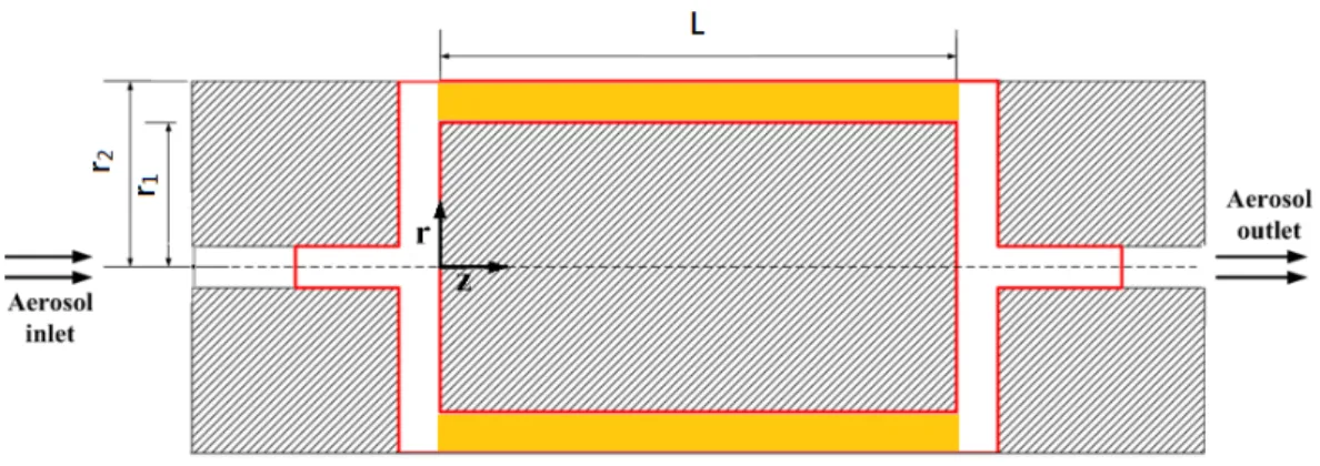
Calculation Domain
Fig. 9. The extended calculation domain (dark orange area) (Kanomax Inc.)
Fig. 9 shows the detailed geometry of the APMs. The dark orange area indicates the extended calculation domain. All regions where particles would pass through are considered in the model.
27
Flow Field
Instead of applying parabolic flow field for the velocity profile, the velocity profile in the calculation domain is calculated with the Navier-Stokes equations (Eq. (36)~(38)) and the continuity equation (Eq. (39)). We consider that the flow filed in the APM is steady. It is assumed that velocity would not change in the θ direction, which makes the 2-D consideration for the flow field available. Noted that uθ, described by Eq. (40), appears in the Eq. (36). It reveals that the velocity in r direction (ur) is affected by the rotation speed. Su in the Eq. (38)
is considered as the source term as described in Eq. (41). Since we consider the particles flow as the incompressible fluid, the continuity equation (Eq. (40)) is available to be applied to the flow field model.
ρgas�ur∂u∂rr+ uz∂u∂zr� = −∂P∂r+ µgas�∂
2ur ∂r2 + 1 r ∂ur ∂r + ∂2ur ∂z2� + ρuθ2 r − µur r2 (36)
ρgas�ur∂u∂rz+ uz∂u∂zz� = −∂P∂z+ µgas�∂
2uz ∂r2 + 1 r ∂uz ∂r + ∂2uz ∂z2� (37)
ρgas�ur∂u∂rθ+ uz∂u∂zθ� = −1r∂P∂θ+ µgas�∂
2u θ ∂r2 + 1 r ∂uθ ∂r + ∂2u θ ∂z2 � + Su (38) 1 r ∂ ∂r�ρgasrur� + ∂ ∂z�ρgasuz� = 0 (39) uθ = ωr (40) Su = −ρurruθ−µur2θ (41)
The equations are discretized by the finite volume method. The SIMPLER algorithm (Semi-Implicit Method for Pressure-linked Equation) (Patankar 1980) is used to solve the equations numerically (Lin et al., 2010). The numerical results of the flow field are applied to the advanced model for the calculation of the transfer function.
28
3.4 Simplified Model
Before applying model with detailed flow field to calculate the transfer function, the user has to spend lots of time on calculating the velocity profile of the field. Moreover, because the velocity profile is dependent on the rotation speed, flow rate and geometry of the APM, we have to calculate the velocity profile for each different operating condition. After that, we have to spend more time on calculating the transfer function. To simplifying the calculation process, the study develops the fitting model based on the numerical results to calculate transfer function in more efficient manner. Moreover, the study also applied numerical results to develop the modified Ehara model, which can calculate the transfer function as analytical solution. The two methods are described in following sections.
Fitting Model
The study builds up a fitting model, which is based on the numerical results simulated by the model with extended domain and detailed flow field. Gaussian distribution, as described in Eq. (42), is applied to fit the transfer function simulated by the developed numerical swirl model. Particle classified by the APM is considered to be spherical and singly charged, so the specific mass of particle can be easily converted to the diameter dp.
dΩAPM�dp, ωλc, V� = σ√2πX exp �−(V−Vc)
2
2σ2 � dV (42)
In Eq. (42), ΩAPM�dp, ωλc, V� is the transfer function of the particle, whose diameter is dp, passing through the APM operated with rotation speed ωλc and voltage V. ωλc is the
rotation speed determined based on the size of center particle (dp,c) and the chosen λc (Eq. (4)),
and V is the voltage applied to the APM. is the standard deviation of the voltage range that enable particle with diameter dp to pass through the APM without being removed when
29
the rotation speed is fixed at ωλc. The value of is obtained by trail and errors until the maximum difference between the fitted ΩAPM�dp, ωλc, V� and numerical ΩAPM�dp, ωλc, V� is
minimized. Moreover, X is the correction factor, which not only normalizes the Gaussian distribution but also makes the maximum height of the Gaussian distribution equal to the maximum height of the numerical transfer function. Vc is the center voltage, derived from
the rotation speed ωλc through equation. ΩAPM�dpc, ωλc, Vc� is the maximum transfer
function when the APM is operated with ωλc and Vc. If the terms of σ and X are known, we can calculate the transfer function through Eq. (42) without additional numerical calculation.
Table 4 The results of fitting numerical transfer function with Gaussian distribution.
Gaussian Distribution Fits Numerical Models For APM-3600, 1 lpm, λc=0.22
dp(nm) σ Vc
Max abs. Error (in T.F.) Sum of abs. Errors (in T.F.) X σ/Vc Vc/σ 20 0.399 2.10 0.032 0.290 0.284 0.190 5.263 30.6 0.800 4.79 0.026 0.150 0.989 0.167 5.988 51 2.150 12.70 0.050 0.525 3.407 0.169 5.907 100 6.690 43.24 0.027 0.270 12.694 0.155 6.463 208 20.840 143.63 0.026 0.170 42.029 0.145 6.892 479 63.330 454.17 0.026 0.320 130.071 0.139 7.171 791 115.910 832.75 0.028 0.380 239.431 0.139 7.184
In this section, the study chose the case of applying the APM-3600 to measure the mass distribution of particles with 0.22 of λc and 1 lpm of flow rate. Gaussian distribution is
applied to fit seven different numerical transfer functions, which are simulated for particles with diameter 20 nm, 30.6 nm, 51 nm, 100 nm, 208 nm, 479 nm, 791 nm respectively. The
30
parameters, σ and X, is determined by trail and errors to minimize the maximum difference between the numerical transfer function and fitting Gaussian distribution. The obtained and X for each transfer function are listed in table 4. T.F. shown in table 4 is the abbreviation of the transfer function. The and X shown in table 4 are further fitted to predict the σ and X for size of particle which is not converted by the table. The fitting equation of and X are shown as below. The parameters, A,B,C,D,E, shown in Eq. (43)~(48) are listed in table 5 respectively. To remain the accuracy of the prediction, the digits of parameters after decimal point should not be rounded off.
Fitted σ: For 208 nm > dp > 17 nm, σ = A × e�B×dp�+ C × e�D×dp�+ E. (43) For 791 nm > dp > 208 nm, σ = A × e�B×dp�+ C × e�D×dp�+ E. (44) For dp > 791 nm, σ = 0.139 × Vc. (45) Fitted X: For 208 nm > dp > 17 nm, X = A × e�B×dp�+ C × e�D×dp�+ E. (46) For 791 nm > dp > 208 nm, X = A × e�B×dp�+ C × e�D×dp�+ E. (47) For dp > 840 nm X = 239.431 + 0.3505126 × (dp− 791). (48)
31
Table 5 The parameters of equations which are applied to fitted the obtained and X.
Fitted σ Fitted X 208 nm > dp > 17 nm 791 nm > dp > 208 nm 208 nm > dp 840 nm > dp > 208 nm A 17.9219737 A 83.6538647 A 77.0379673 A -6.9615277 B 0.0039508 B 0.0017356 B 0.0024631 B 0.0037867 C 2.9876668 C -11.6140818 C 10.0264075 C 169.7009613 D -0.058499 D 0.0031225 D -0.0259945 D 0.0014929 E -19.9238423 E -76.9483039 E -86.6056268 E -174.1644899
Fig. 10. Comparison between the numerical transfer function (solid lines) and the transfer function predicted by the fitting model (dashed lines)
To verify the fitting model, the transfer functions determined by the fitting model are compared with the fitted numerical transfer function. Fig. 10 shows the results of the
32
comparison. Good agreements are obtained and considered the verification of the fitting model. It should be keep in mind that because the fitted numerical transfer functions are simulated for the APM-3600 which is operated with 0.22 of the λc and 1lpm of the flow rate,
the parameters shown in this section is only available for the APM-3600 operating with the same condition.
Modified Ehara Model
The study develops a modified Ehara model to calculate the transfer function as exact solution with considering the effects of Brownion motion. The model combines the model developed by Ehara et al., (1996) and the modified Gormley and Kennedy equation, which is modified based on our numerical results.
Ehara et al., (1996) developed a model (Ehara model) to calculate the transfer function of particles classified by the APM based. With the assumption of uniform flow field in the classifying region of the APM, Ehara model can calculate the transfer function as exact solution. Moreover, when the λc is sufficient low, the transfer function calculated with the
uniform flow field can be very similar to the one calculated with the parabolic flow field, which is more close to the real flow field (Fig. 7). Hence, Ehara model was available to calculate the transfer function as exact solution without considerable error for the APM operated with low value of λ.
Fig. 11 is the typical transfer function calculated with the Ehara model with the uniform flow field. In Fig. 11, the shape of the transfer function can be determined by four special specific masses S1+, S1-, S2+, S2-. These specific masses can be calculated with Eq. (49) and
(50) (Ehara et al., 1996). Sc is the specific mass of center particle (Eq. (51)), which achieves
force balance of centrifugal force and electrostatic force at the center position (r=rc) between
33
Fig. 11. Four particular specific masses
S2±≈ Sc�1 ± 2rδc� (49) S1±≈ Sc�1 ± 2 �rδc� coth �λ2c�� (50) Sc =r V c 2ω2ln�r2 r1� (51)
Based on the specific mass S of particle, the transfer function ΩAPM(S) can be determined
by three equations. If S ranges between S1− and S2−, ΩAPM (S) can be calculated with Eq.
(52). Similarly, if S ranges between S2− and S2+, ΩAPM (S) can be determined by Eq. (53).
If S ranges between S2+ ≤ S ≤ S1+, ΩAPM (S) can determined by Eq. (54). If S is out of these
ranges, particle with such S will be completely removed by the APM.
For S1− ≤ S ≤ S2− (ρ0h = 1)
ΩAPM(S) =12�[1 − ρ(S)] + [1 + ρ(S)]e−λ� (52)
For S2− ≤ S ≤ S2+
34
For S2+ ≤ S ≤ S1+ (ρ0l = −1)
ΩAPM(S) =12�[1 + ρ(S)] + [1 − ρ(S)]e−λ� (54)
ρ(S) in Eq. (52)~(54) is the position of particles expressed in normalized coordinate as described by Eq. (55) and (56). r(S), derived from Eq. (1) is the position where centrifugal force and electrostatic force acting on particle of specific mass S are the same.
ρ(S) =[r(S)−rc] δ (55) ζ =Lz (56) r(S) = �Sω2Vln�r2 r1� (57)
To apply the Ehara model with considering the effects of Brownian motion, the study applied Gormley-Kennedy equation (Eq. (58)~(60)) to consider the effects of the Brownian motion of particles on the transfer function. It is assumed that the diffusion loss of particles is independent to the classification of the APM. In other words, the study applies the product of ΩAPM (S) and PG&K to calculate the transfer function of nanoparticles. In the study,
Ehara model modified by the diffusion loss equation is denoted as the Modified Ehara model, and the transfer function calculated with the modified Ehara model is denoted as Ω’APM(S).
µ =πDL(r2+r1)
Q�(r2−r1)� (58)
PG&𝐾 = 1 − 2.96µ
2
3+ 0.4µ for μ<0.005 (59) PG&𝐾 = 0.910 exp(−7.54µ) + 0.0531exp(−85.7µ) for μ≧0.005 (60)