解析台灣教育的效果與功能---個體與總體分析

行政院國家科學委員會專題研究計畫 成果報告

解析台灣教育的效果與功能: 個體與總體分析(第 2 年)

研究成果報告(完整版)

中 華 民 國 99 年 03 月 29 日

Summary of final report

In this research project, I have tried to identify what’s the “true” rate of return to education in Taiwan. Using Instrumental variable method and heterogeneous human

capital theory, I had developed three empirical models to estimate and discover the rate of return to education in Taiwan. The main sources of data are from varies years

of Taiwan’s Manpower Utilization Survey. As education is an important form of human capital accumulation, can education be also an effective means for fostering

intergenerational social mobility? Using Taiwan’s Panel Study of Family Dynamics data, I also investigate education and intergenerational social mobility in Taiwan.

The major conclusions from my research are that the estimated rates of return to education are relatively higher by the IV method than by the OLS method. The

estimated rate of return to education is 5.97% for males and 14.69% for females, higher than that by OLS especially in the female group. Due to the severe influence

by family factors on females’ education, we also find that the female rate of return to education is significantly underestimated the by OLS. The Taiwan empirical study

also shows that significant heterogeneous return to education does exist and the educational choice was made according to the principle of comparative advantage.

The estimated rates of return for attaining university were 19% and 15%, much higher than the average rate of return of 11.55 and 6.6%, for 1990 and 2000, respectively.

The decline trend of return to university education may be caused by the rapid expansion of the number of colleges and universities and the increasing supply of

college graduates in the 1990s. Quantile regression with cohort data also confirms the same result. Moreover, we find that education and ability are complements for the old

cohort, while they are substitutes for the young cohort, i.e., education can compensate disadvantage in ability. The important policy implication is that general education

may consolidate and even create social diversity.

Empirical results from PSFD data find that father’s social status affects an

individual’s educational attainment. Offspring whose father is in the upper class have the best advantage of receiving higher education than those whose father is not.

Moreover, education has a profound influence on social status. The higher the educational attainment is, especially for university and above, the greater the chance

will be in the upper-class and the advantage of education to enter the upper class does not vary among different cohorts. This implies that the upper-class may dominate

education to preserve their social status. However, other things being equal, for those with junior college education but their fathers are not in the upper-class, tend to have

a greater chance to be in the upper-class than those whose father is in the upper-class. Hence, education can still be an effective means to compensate the disadvantage in

one’s father’s social status. We also find that senior high school and junior college education has the greatest chance to be in the middle class, which is conducive to

social stability. Our results confirm that popularization of education is beneficial to intergenerational social mobility. Thus, equal opportunity to attain education and

prevention of monopoly in education by the upper class should be the ultimate goal of a government’s educational policy as it not only enhances one’s earning capability but

also fosters social mobility.

The above research has developed into four papers: 1. Endogeneity and

Investment in Education: Estimating Rates of Return to Education for Taiwan, 2. Heterogeneity, Comparative Advantage, and Return to Education: The Case of

Taiwan, 3. Return to education and ability in Taiwan: an cohort analysis, 4. Education and Social Mobility in Taiwan. The following attachment is the complete version of

Endogeneity and Investment in Education: Estimating Rates of

Return to Education for Taiwan

Abstract

To avoid the endogenous bias of the education variable in the OLS estimation of return to education, this paper applies the 2SLS instrumental variable method to estimate the rate of return to education using data from the 1990 Taiwan’s Manpower Utilization Survey. Instrumental variables include the nine-year compulsory education policy, area of residence, sibling status, and father’s education. Tests are also conducted to choose the most effective valid instrument from all combinations of IVs. Consistent with the literature, the estimation results show that the estimated rate of return to education is relatively higher by the IV method than by the OLS method. Due to the severe influence by family factors on females’ education, we also find that the female rate of return to education is significantly underestimated by the OLS.

Keywords: Human capital investment, return to education, endogenous bias, ability bias, instrumental variable, local average treatment effect

Endogeneity and Investment in Education: Estimating Rates of

Return to Education for Taiwan

I. Introduction

Human capital investment and accumulation have been identified as one of the

important sources for a country’s long-run economic growth.1 For the past four

decades, Taiwan, a small island of 36,000 kilometers with limited natural resources,

has achieved the so-called “economic miracle” with average annual economic growth

rate of 8.45% between 1960 to 2000. Taiwan’s remarkable economic performance is

consistent with the human capital theory to a large extent due to the development of a

well-educated and better-trained labor force, which speeds up industrialization

processes and upgrading of technology to sustain the long-run growth of the economy.

Chuang (1999) finds that during the 1964-1994 period, 30% of Taiwan’s average

annual economic growth can be attributed to human capital. Lin (2004) also discovers

that higher education had a positive effect on economic growth in Taiwan for the

period 1965-2000; one additional percent of higher education stock is estimated to

increase real output by approximately 0.19%. Moreover, examining the relation

between education and growth, Chuang (2000) finds that unidirectional causality runs

from higher education to economic growth in Taiwan over the period 1952-1995. Wu

(2003) notices an increasing trend of rates of return to education in Taiwan from 1978

to 2001.

These findings on the education-growth nexus of Taiwan’s economic miracle can

be described as follows. Since the adoption of an open trade policy in the early 1960s,

Taiwan has experienced drastic and rapid structural changes from an

agriculture-oriented to an industry-oriented economy. In fact, the output share of

industry increased from 23.03% in 1961 to 39.36% in 1978, subsequently remaining

relatively stable until the mid 1980s. The structure of exports changed from

labor-intensive products in the 1960s, to capital-intensive in the 1970s and

technology-intensive in the 1980s. This open trade and rapid industrialization process

increased the demand for skilled labor, which increased the return on education, and

the increase in the quality of workers facilitated the process of accessing, absorbing,

and applying technology upgrades and thus the subsequent economic growth.

The Human capital theory emphasizes education and on-the-job training to

enhance labor productivity and hence wage rates of workers.2 _{The economic return to}

education not only influences an individual’s educational choice but also affects the

labor quality of the whole society. Therefore, from both individual and social points

of view, the estimation of return to education is an important measure for human

capital investment decisions and thus has a profound effect on human development.3

For the past forty or more years, investment in education has expanded greatly in

Taiwan due to the government’s expansionary education policy, the process of rapid

industrialization, and the conventional wisdom that “To be a scholar is to be at the top

of society.” The average years of education for employed workers in Taiwan has

increased tremendously from 7.18 years in 1978 to 11.03 years in 2006, while for the

same period, the per capita income rose from US$1,461 to US$14,455, a roughly

ten-fold increase. According to the human capital theory, education enhances labor

productivity and hence increases wage rates. But what is the economic return for an

additional year of schooling? Previous empirical studies on returns to education in

Taiwan, e.g., Psacharopouls (1985); Gindling, Goldfarb, and Chang (1995); Chuang

and Chao (2001); and Wu (2003), among others, have neglected either the

endogeneity problem of education or the heterogeneity of unobserved ability, thus

tending to encounter the endogeneity bias and ability bias for the estimates of returns

to education.4 _{Two exceptions are Gurgand (2003) and Spohr (2003), who adopted}

3 _{Return to education is one of important measures in constructing the human development index,}

which is considered to be a more inclusive index for measuring human welfare and has been announced every year by the United Nations since 1990.

4 _{The former is caused by educational decisions and is endogenous rather than exogenous, and the}

the IV method, but with a simple instrumental variable or special attention to specific

groups only. Gurgand (2003) estimates the influence of education on a farmer’s

income, adopting a simple instrumental variable of the share of primary and high

school farmers to replace the formal years of education, while Spohr (2003) uses the

nine-year compulsory education policy as the instrumental variable and adopts the

yearly wage instead of the hourly wage as the dependent variable.5 _{Instead of using a}

single instrumental variable, this paper intends to deal with the problems by using

four different instrumental variables, namely the nine-year compulsory education

policy, area of residence, sibling status, and father’s education, and their combinations,

to identify an unbiased and consistent estimate of the rate of return to education for

Taiwan. Tests of the validity of various combinations of instruments are conducted.

We find that the combination of the compulsory education policy and area of

residence is the most efficient valid instrument and may give a better estimation for

the rate of return to education.

Due to the heterogeneity of an individual’s ability, the conventional OLS

estimation of the wage equation will be subject to the ability bias because the

intercept of the wage equation by the OLS method reflects personal ability, which is

correlated with the marginal cost of receiving education. Moreover, if the

heterogeneity of an individual’s ability is revealed by the different slopes of the wage

equation, i.e., the greater the return to education, the higher the incentive for

educational investment, then under this situation, the estimation results by the OLS

method will be further inflated. As there exist heterogeneous returns to education,

reflected by the intercept and slope of the wage equation, the adoption of the OLS

method to estimate the return to education requires that explanatory variables and the

error term be mutually independent. Failure to satisfy this condition will render a bias

in estimation by the OLS method. More importantly, educational investment is an

endogenous decision process that is heavily influenced by personal characteristics and

family background factors. As the education variable is not exogenous, conventional

OLS estimation will be subject to bias.6

Griliches (1977) proposes to use the instrumental variable method to tackle the

problems of ability bias and endogeneity.7 _{However, the major difficulty is to find a}

valid instrumental variable, especially for cross-section data analysis such as the

estimation of return to education. Heckman and Vytlacil (1999) point out that the

instrumental variable has to be correlated with an individual educational choice and

6 _{For discussion of factors that determines an individual’s educational choice, see, for example,}

Haveman and Wolfe (1995).

7 _{Griliches (1977) uses the viewpoint of the efficiency unit in the labor market and considers human}

capital to be homogenous; thus, people choose to have different stocks of human capital. In this regard, to solve for the problems of ability bias and measurement error, an effective estimation method is the instrumental variable method. Sometimes this type of model is also called the common coefficient

uncorrelated with an individual’s ability. Most of the existing literature has shown

that it will be relatively difficult to find a valid instrumental variable from the demand

side of education, as we are not quite certain that the demand factor for education has

no correlation with an individual’s wage rate. Therefore, economists are inclined to

use supply factors for education such as family background factors as the instrumental

variable. For example, Trostel, Walker and Woolley (2002) use parents and spouse’s

education as instrumental variables to estimate male and female return to education

for 28 countries, finding that the estimated rate of return to education is typically

higher when calculated by the IV method than by the OLS method. Other studies,

such as Arcand, D’hombers and Gyselnck (2004), Patrinos and Sakellariou (2005),

and Sakellariou (2006), adopt the father’s years of education as the instrumental

variable; all of these find results similar to those of Trostel, Walker and Woolley

(2002).8

As we are not convinced that family background factors are uncorrelated with an

individual’s ability, recent studies have switched to supply side factors of the labor

market as the instrumental variable.9 _{For example, Angrist and Krueger (1991) use}

8 _{See Card (2001) for a detailed comparison and discussion of the estimation results by OLS and IV}

methods.

9 _{If there is an inter-generational transfer effect, family background factors such as parents’ education}

birth season as the instrumental variable, as differences in birth season cause different

dates of school enrollment and hence different times for completing compulsory

education. Apparently, birth season has a correlation with years of schooling, but

none with an individual’s ability. Harmon and Walker (1997) use the compulsory

educational policy in the U.K. as the instrumental variable because the change in

educational policy is exogenous but in fact influences people’s minimum years of

schooling. As the instrumental variable is subject to the educational choice of

particular demographic groups, the results estimated by the IV method can be

interpreted as the marginal rate of return to education for those particular

demographic groups. Likewise, the estimated rate of return to education for the IV

method is usually higher than that for the OLS method.10

There are other instrumental variables in the literature. For instance, Duflo (1999)

chooses birth date before and after institutional change, and personal residential area,

as the educational resources may be different under different policies, as instrumental

variables. Moretti (2004) uses estimated demographic structure in the city and

land-grant university as instrumental variables to estimate estimated spillover effect of

education and social rate of return to education.

10 _{Card (2001) has an alternative interpretation. He thinks that people with low education tend to have}

Conventionally, under the assumption of mutual independence of the explanatory

variables and the error term, estimates from the OLS method are interpreted as the

average marginal rate of return to education. However, if it is not the case, as it

usually is, the OLS estimates will subject to the endogeneity bias.

Based on the results from the literature, this paper intends to estimate the rates of

return to education for Taiwan. The major contributions of the paper are to take the

endogeneity of education and the individual’s heterogeneity into account to estimate

an unbiased and consistent rate of return to education using the IV method. Second,

tests are conducted to choose the most effective valid instrument from all

combinations of IVs. Third, conducting a case study of Taiwan, a country

characterized by an economic miracle with rapid accumulation in education

investment, may provide useful implications for other developing countries.

This paper is organized as follows. Section II specifies the empirical model.

Section III contains data description, estimation results, and sensitivity analysis. The

conclusion follows in Section IV.

As in the literature, we use Mincer's (1974) specification of wage equation as the

basic model for the estimation of rate of return to education, and an additional

educational choice equation is also stated as

i i i X S u Y = ′δ +β + , i i i Z v S = 'α + ,

where Y is the real hourly wage in logarithmic form; X is other variables

affecting an individual’s wage rate, such as work experience, marital status, industry,

and firm size; S denotes years of schooling; Z is explanatory variables including

instrumental variables that determine one’s educational choice; u and v are error

terms for wage and educational choice equations, respectively; and the coefficient β represents the average rate of return to education for additional years of schooling.

To cope with the endogeneity problem of investment in education, a 2SLS

instrumental variable estimation method is used. Furthermore, as the samples are

subject to those who work for a wage payment, the direct estimation of the wage

equation will encounter the problem of sample selection bias. Thus, we adopt

Heckman’s (1976) two-stage selection model to explicitly correct for the problem of

selection bias.11

The selection of instrumental variables

The use of instrumental variables to estimate return to education requires that

instrumental variables satisfy the orthogonality condition; i.e., instrumental variables

have no correlation with the individual’s ability or error term. Furthermore, under the

heterogeneous return to education, instrumental variables have to be uncorrelated with

one’s earning capability in addition to the orthogonality condition; i.e.,

Z

uncorrelated with β . In other words, allowing for a heterogeneous return to education, the instrumental variable should be correlated with one’s educational

choice, but uncorrelated with one’s wage rate.12

We first adopt the nine-year compulsory education policy as our instrumental

variable. Numerous studies have shown that the compulsory educational policy has a

significant effect on return to education; see, e.g., Angrist and Krueger (1991); Cruz

and Moreira (2005); and Sakellariou (2006), among others. From a policy perspective,

the implementation of a compulsory educational policy significantly enhances the

structure of labor quality of the developing countries, especially for those groups

subject to family liquidity constraints.13 Thus, the use of the compulsory educational

12 _{See, for example, Blundell et al. (2003) for detailed discussion on this point.}

policy as the instrumental variable not only solves for problem of endogeneity and

ability bias caused by the OLS method but also gives us estimates for the rate of

return to education for those who are subject to liquidity constraints, an important

factor that hinders educational investment for economically disadvantaged people.

Most research on return to education in developing countries has proved that using

institutional factors as the instrumental variable tends to result in a higher estimated

rate of return to education than that found by the OLS method.14

Compulsory educational policy is an institutional change that includes the

building of new junior high schools and recruitment of new educational staff and

teachers, and thus it is closely related to an individual’s educational investment but

has no direct relationship with an individual’s ability. As educational resources are

different among different residential areas, it thus has different impacts on

individual’s educational achievement, while having nothing to do with an individual’s

ability. From the viewpoint of the life cycle of household income, elder children tend

to have less family education resources than their young siblings do, as family income

is usually low in the early stage.15 _{Moreover, the greater the number of siblings for a}

to credit constraints.

14 _{See, for example, Card (2001) for a detailed literature review on this line of research.}

15 _{Using data from the 1989 Survey of Women's Living Status in the Taiwan Area, Parish and Wills}

given family budget constraint, the fewer the educational resources that are given to

each child. Thus, both the existence of young siblings and the number of such siblings

will be correlated with an individual’s educational achievement, but these factors have

no correlation with an individual’s ability or wage. Therefore, this paper adopts the

nine-year compulsory education policy, residential area, and the existence of younger

siblings as instrumental variables for educational choice.16 _{In the literature, some}

research, see, e.g., Trostel, Walker and Woolley (2002); Arcand, D’hombers and

Gyselnck (2004); Patrinos and Sakellariou (2005); and Sakellariou (2006), among

others, use family background variables such as the father’s education as the

instrumental variable; for comparison, we thus also include father’s education as an

additional instrumental variable.17

Tests of validity for instrumental variables

Econometrically, in the 2SLS estimation, a valid instrumental variable should

satisfy two conditions: Instrument relevance and Instrument exogeneity. The relevant

tests include using the partial coefficient of determination or F-test to test the

explanatory power and sign of the instrumental variable on the endogenous education

16 _{We also regard the number of siblings as the instrumental variable; the estimated results are similar}

to what we have reported here.

variable at the first step of regression.18 _{As for the exogeneity test, the}

over-identifying restrictions test is used on the orthogonality condition for all the

instruments.19 _{In the second stage of regression, we adopt the Durbin-Wu-Hausman}

test for exogeneity.20

III. Data analysis and estimation results

As the paper uses the nine-year compulsory educational policy, which was

implemented in Taiwan in 1968, as one of the instrumental variables for a broader

inclusion of samples, we adopt data from the 1990 Taiwan Manpower Utilization

Survey conducted by the Directorate-General of Budget, Accounting and Statistics,

Executive Yuan, Taiwan, Republic of China.21 The MPUS data are repeated cross

18 _{See Bound, Jaeger, and Baker (1995) and Staiger and Stock (1997) for detailed descriptions of the}

relevant tests. The F-test can be used to joint test the significance of coefficients of all the instrumental variables. A rule of thumb is that F statistics should be greater than 10, and that any values below 10 imply that the selected instrumental variables have insignificant explanatory power and thus generate estimation bias.

19 _{Assume that the number of selected instruments is m and the number of relevant endogenous}

variables is k. If m=k, the regression coefficients are exactly identified. If m>k, the regression coefficients are over-identified. If m<k, the regression coefficients are under-identified.

20 _{The estimation process is similar to test for the omitted variable, as it was first proposed by Durbin}

(1954), Wu (1973), and Hausman (1978), respectively; hence it is also called the Durbin-Wu-Hausman (DWH) test. For a discussion of DWH test of exogeneity, see, for example, Davidson and MacKinnon (2003).

21 _{We also tried the Taiwan Manpower Utilization Survey data for 1995 and 2000. The results are}

similar to what we report in this paper. However, data for the 1995 and 2000 MPUSs may encounter limited sample problems. For example, the proportion of samples having received nine-year compulsory education is as high as 95% and 99% for 1995 and 2000, respectively. Thus, the use of the nine-year compulsory educational policy as the instrumental variable for 1995 and 2000 data will be subject to insufficient samples of those who were not affected by the compulsory education policy. For

sections and stratified random samples of around 20,300 households (about 60,000

persons aged 15 and above in these sampled households) from about 532 villages and

neighborhoods in Taiwan, and they are not panel data. For the use of instrumental

variables, we choose samples only with complete intergenerational information, such

as father’s education and number of siblings. A total of 7,193 samples are obtained.22

Tables 1 and 2 present all the variable names, definitions, and basic statistics.

22 _{As the samples with complete intergenerational information are smaller than the original survey}

samples, then to ensure the representation property of the selected sample, we further conducted conventional OLS estimation for return to education for our selected sample and the original survey sample, finding that the estimation results for the two samples are similar, which justifies the

Table 1. Variable name and definition Name Definition

Wage Real hourly wage in logarithmic form. Years of

education Education levels include illiterate and self educated, primary school, junior high school, senior high school, vocational school, junior college, university, graduate school and above. The corresponding years of education are 0, 6, 9, 12, 12, 14, 16, and 18 years, respectively.

Tenure Years working at current job. Work

experience Work experience is proxied by age-years of education-6-tenure. As males in Taiwan need to serve two years in the army, an additional 2 years is thus further subtracted for males.

Sex Dummy variable: 0 for female, 1 for male. Marital status Dummy variable: 0 for single, 1 otherwise.

Industry Industry in which the individual works are dummy variables, which include agriculture, forestry, fishery, and husbandry; manufacturing; water, electricity, fuel, and coal; construction; wholesalers, retailers, and restaurants; transportation, storage, and communications; finance, insurance, and real estate; and public and personal services. Wholesalers, retailers, and restaurants is the reference group.

Firm size Dummy variables include 1-9 persons, 10-49 persons, 50-99 persons, 100-499 persons, 500 persons and above, and the public sector. 1-9 persons is the reference group.

Residential

area Residential area is classified into urban and rural areas and represented by a dummy variable: 0 for rural area, 1 for urban area. Based on the official classification of Taiwan’s Ministry of Interior, cities, towns, or villages with a population of residences of over fifty thousand are classified as urban areas.

Number of

siblings Having younger siblings in the family is represented by a dummy variable: 1 for yes and 0 for no. Compulsory

educational policy

People affected by the nine-year compulsory educational policy implemented in1968. A dummy variable: 0 for those who were born before 1956 (not affected by the policy) and 1 for those who were born after 1956 (affected by the policy).

Table 2. Summery of basic statistics for variables Variable name Mean Standard

Deviation value Min. value Max.

Age 27.79 6.81 15 64 Years of education 10.83 2.76 0 18 Tenure 3.55 4.17 0.08 41.17 Work experience 6.09 5.70 0 46 Sex 0.66 0.47 0 1 Marital status 0.32 0.47 0 1 Industry Agriculture 0.05 0.21 0 1 Manufacturing 0.38 0.49 0 1 Water, electricity,

fuel, and coal 0.01 0.07 0 1

Construction 0.11 0.31 0 1 Wholesalers, retailers, and restaurants 0.18 0.39 0 1 Transportation, storage, and communications 0.06 0.23 0 1 Finance, insurance, and real estate 0.05 0.23 0 1 Personal and public services 0.17 0.37 0 1 Firm size 1-9 persons 0.44 0.50 0 1 10-49 persons 0.26 0.44 0 1 50-99 persons 0.07 0.26 0 1 100-499 persons 0.11 0.31 0 1 500 persons and above 0.04 0.19 0 1 Public sector 0.09 0.28 0 1 Instrumental variable Educational policy (IV1) 0.86 0.35 0 1 Residential area (IV2) 0.68 0.47 0 1

Number of

Siblings (IV3) 0.26 0.44 0 1

Father’s

education (IV4) 6.05 3.86 0 18

Observations 7193

Source: 1990 Manpower Utilization Survey, DGBAS, Taiwan

Industry includes 8 one-digit and 76 two-digit classifications, according to the

Standard Classification of Industry of the Republic of China, DGBAS.23 Residential

area is classified into urban and rural areas. Based on the official classification of

Taiwan’s Ministry of the Interior, cities, towns, or villages with over fifty thousand

residences are classified as urban areas. Due to data limitations, it is not possible to

acquire residence information for samples during their study period. We use current

residence as a proxy for the residence during schooling age.24

The total sample is 7,193 persons, average age is 28 years old, average years of

education is 10.83 years, with an average tenure of 3.55 years and work experience of

6.09 years. Among them, females comprise 34% and males 66%; 23% are married;

38% work in manufacturing, 18% in wholesalers, retailers, and restaurants; 17% in

23 _{The original classification of industry includes 9 one-digit and 85 two-digit industries, for simplicity}

and research purposes, we had aggregated some industries, which results in 8 one-digit and 76 two-digit industries.

24 _{A possible bias from this assumption is that current residence may not be the same as the residence}

of schooling age, i.e., the residence of schooling age was in a rural (urban) area, but current residence is in an urban (rural) area. However, according to data from Panel Study of Family Dynamics, conducted by Academia Sinica since 1999, for those who were born between 1953 and 1963, the percentage of those living in rural areas during their schooling years but currently living in urban areas is 1.23%, while that for those living in urban areas during their schooling years but currently living in rural areas

personal and public services; 70% worked at small- and medium-size firms (below 50

persons); only 4% worked at large enterprises (500 persons and above); and 9%

worked in the public sector; 86% received nine-year compulsory education; 68%

lived in urban area and 32% in rural area.

Estimation results

We use the IV method or so-called 2SLS method to estimate rate of return to

education for Taiwan. The results of first stage regression for educational choice are

presented in Table 3. The four instrumental variables, educational policy (IV1),

residence area (IV2), number of siblings (IV3), and father’s education (IV4), as

expected, all have a positive effect on individual’s education achievement. These

results imply that those who receive compulsory education, live in urban areas, have

no younger siblings, and have fathers with higher education tend to have more

education. Moreover, even including all four instrumental variables into the

educational choice regression, as in column 5 of Table 3, the estimated coefficients all

remain significant and have expected signs.

IV1 IV2 IV3 IV4 IV1+IV2+IV3+ IV4 Age 0.4908*** 0.4883*** 0.4809*** 0.4473*** 0.3958*** (17.59) (17.85) (16.73) (17.52) (15.12) Age2 -0.0083*** -0.0089*** -0.0088*** -0.0079*** -0.0066*** (-18.68) (-21.33) (-20.10) (-20.21) (-15.77) Educational policy 0.9974*** 0.9635*** (6.75) (7.17) Residence area 1.1235*** 0.7144*** (16.47) (11.15) Number of siblings -0.3104*** -0.2150*** (4.17) (3.18) Father’s education 0.2764*** 0.2592*** (37.33) (34.75) Constant 3.2259*** 3.8294*** 4.5216*** 3.2363*** 2.1664*** (6.98) (8.93) (10.29) (8.09) (5.09) Partial R2 0.0057 0.0327 0.0022 0.1460 0.1647 F-test 19.6*** _67.7*** _11.4*** _579.4*** _609.1*** Adj-R2 0.1063 0.1333 0.1028 0.2466 0.2650 Observations 7193 7193 7193 7193 7193

Notes: 1. Figures in the parentheses are t statistics.

2. *, **, and *** stand for statistical significance levels at 90%, 95%, and 99%, respectively. 3. The F-test is for the instrument relevance condition (the significance of coefficients of all the

instrumental variables). A rule of thumb is that F statistics should be greater than 10, and that any values below 10 imply that the selected instrumental variables have insignificant

explanatory power and thus generate estimation bias.

To ensure that our instrumental variables are valid instruments, we further test for

determination and the F-test of first stage regression in Table 3, all four instrumental

variables have significant correlations with years of education. Among them, the

father’s education has the most explanatory power for an individual’s education. As

for the exogeneity test, from Table 4, the over-identifying restrictions test shows that

the four instruments are not all exogenous, suggesting that potential endogeneity

within the four instruments may bias the estimation.25

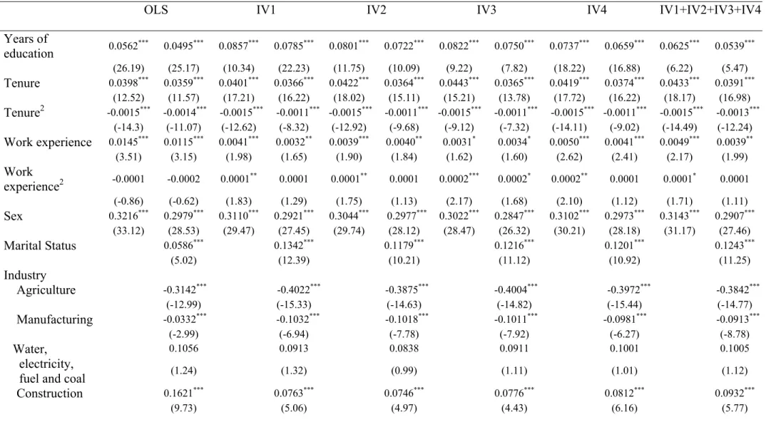
Table 4 lists the estimation results for the rates of return to education for the OLS

and IV methods. First, by considering a parsimonious formulation of the Mincerian

wage equation, which includes only variables like tenure and work experience in

addition to education, the estimated rates of return to education, tenure, and work

experience are 5.62%, 3.98%, and 1.45%, respectively. Including additional

explanatory variables, which include marital status, industry, and firm size, the

estimated rates of return to education, tenure, and work experience drop to 4.95%,

3.59%, and 1.15%, respectively. It should be noted that by construction, a valid

instrumental variable should not be correlated with wage or any variable that explains

wage; therefore, in the spirit of the IV method for estimating wage equation, the

omitted variable bias problem should be negligible. We find that those additional

explanatory variables are all significant with the expected signs; in general, those who

are married, work in construction and finance, insurance, and real estate sectors, and

work at large enterprises tend to receive higher wages. Note that from Table 4, the

result of the conventional OLS estimation rejects the null hypothesis of the DWH test

that the education variable is exogenous; hence, this result justifies the use of the IV

method for the estimation of return to education

From Table 4, using the nine-year compulsory education policy (IV1) as the

instrument, the estimated rate of return to education is 8.57%, higher than that found

by the OLS method. This result remains true (7.85% for IV and 4.95% for OLS) even

after controlling for additional explanatory variables. Thus, the estimated average rate

of return to education by the conventional OLS method will be biased downward

because of the endogeneity of education variable. The instrument variable by the

compulsory education policy suggests that compulsory education will increase the

rate of return to education, as the implementation of compulsory education reduces

the marginal cost of education, especially for those children whose families are

subject to credit constraints.

The instrument of residence area (IV2) also shows an estimated rate of return to

education of 8.01%, higher than the estimate found by the OLS. This result implies

to provide more and better educational resources and thus lower marginal costs of

education than rural areas do.

As for the instruments of family background variable, the estimated rates of

return to education for the number of siblings (IV3) and father’s education (IV4) are

8.22% and 7.37, respectively, again higher than that found by the OLS method. This

result implies that one with no younger siblings or a father with more education will

tend to receive more family educational resources, thus resulting in more education

and a higher rate of return to schooling.

However, taking four instrumental variables jointly, the estimated rate of return

to education is still higher for the IV method than for the OLS method but lower than

estimates by any single instrument. The reason is that an estimate using a single

instrumental variable usually represents the rate of return for one particular

demographic subgroup, and as we increase the number of instruments in the first stage

regression, the estimated educational achievement will in general become closer to the

real value and thus approach the average marginal rate of return to education for the

whole group.

Comparing the estimates through four instruments, we find that the estimated

residence area, father’s education, and number of siblings. This result suggests that

institutional factors such as compulsory education have a stronger effect on return to

education than do family background factors such as number of siblings or father’s

education. In other words, as the compulsory education is a comprehensive

institutional change which generally reduces the marginal cost of education for people,

especially those subject to credit constraints, it is thus the most significant effect on

return to education.

Actually, the estimated rate of return to education found by the OLS method is

not the average marginal rate of return to education, or so-called average treatment

effect (ATE); it also encounters the problems of the endogeneity bias and the ability

bias. In contrast, estimates by the IV method not only avoid the problems of the

endogeneity and ability biases but also provide an estimate of the marginal rate of

return to education for a particular demographic subgroup (Card (1999, P.1855)), an

estimate close to the local average treatment effect (LATE) (Heckman, Lalonde, and

Table 4. Estimated rates of return to education: OLS vs. IV

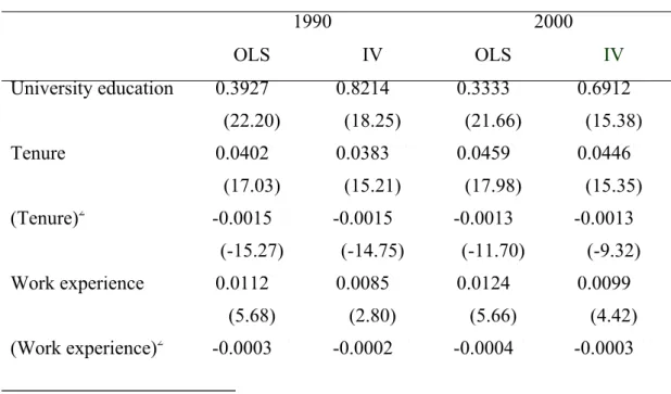
OLS IV1 IV2 IV3 IV4 IV1+IV2+IV3+IV4

Years of education 0.0562*** 0.0495*** 0.0857*** 0.0785*** 0.0801*** 0.0722*** 0.0822*** 0.0750*** 0.0737*** 0.0659*** 0.0625*** 0.0539*** (26.19) (25.17) (10.34) (22.23) (11.75) (10.09) (9.22) (7.82) (18.22) (16.88) (6.22) (5.47) Tenure 0.0398*** _0.0359*** _0.0401*** _0.0366*** _0.0422*** _0.0364*** _0.0443*** _0.0365*** _0.0419*** _0.0374*** _0.0433*** _0.0391*** (12.52) (11.57) (17.21) (16.22) (18.02) (15.11) (15.21) (13.78) (17.72) (16.22) (18.17) (16.98) Tenure2 -0.0015*** _-0.0014*** _-0.0015*** _-0.0011*** _-0.0015*** _-0.0011*** _-0.0015*** _-0.0011*** _-0.0015*** _-0.0011*** _-0.0015*** _-0.0013*** (-14.3) (-11.07) (-12.62) (-8.32) (-12.92) (-9.68) (-9.12) (-7.32) (-14.11) (-9.02) (-14.49) (-12.24) Work experience 0.0145*** _0.0115*** _0.0041*** _0.0032** _0.0039*** _0.0040** _0.0031* _0.0034* _0.0050*** _0.0041*** _0.0049*** _0.0039** (3.51) (3.15) (1.98) (1.65) (1.90) (1.84) (1.62) (1.60) (2.62) (2.41) (2.17) (1.99) Work experience2 -0.0001 -0.0002 0.0001** 0.0001 0.0001** 0.0001 0.0002*** 0.0002* 0.0002** 0.0001 0.0001* 0.0001 (-0.86) (-0.62) (1.83) (1.29) (1.75) (1.13) (2.17) (1.68) (2.10) (1.12) (1.71) (1.11) Sex 0.3216*** _0.2979*** _0.3110*** _0.2921*** _0.3044*** _0.2977*** _0.3022*** _0.2847*** _0.3102*** _0.2973*** _0.3143*** _0.2907*** (33.12) (28.53) (29.47) (27.45) (29.74) (28.12) (28.47) (26.32) (30.21) (28.18) (31.17) (27.46) Marital Status 0.0586*** _0.1342*** _0.1179*** _0.1216*** _0.1201*** _0.1243*** (5.02) (12.39) (10.21) (11.12) (10.92) (11.25) Industry Agriculture -0.3142*** _-0.4022*** _-0.3875*** _-0.4004*** _-0.3972*** _-0.3842*** (-12.99) (-15.33) (-14.63) (-14.82) (-15.44) (-14.77) Manufacturing -0.0332*** _-0.1032*** _-0.1018*** _-0.1011*** _-0.0981*** _-0.0913*** (-2.99) (-6.94) (-7.78) (-7.92) (-6.27) (-8.78) Water, electricity, fuel and coal

0.1056 0.0913 0.0838 0.0911 0.1001 0.1005 (1.24) (1.32) (0.99) (1.11) (1.01) (1.12)

Construction 0.1621*** _0.0763*** _0.0746*** _0.0776*** _0.0812*** _0.0932***

Transportation, storage, and communicatio ns 0.0544*** _{0.0152 0.0151 0.0150 0.0177 0.0163} (3.14) (0.64) (0.75) (0.66) (1.09) (0.95) Finance, insurance, and real estate 0.1121*** _0.1522*** _0.1512*** _0.1561*** _0.1492*** _0.1422*** (4.72) (6.92) (7.01) (7.44) (6.98) (6.43) Personal and public services -0.0251* -0.0438*** -0.0427*** -0.0387** -0.0412*** -0.0402*** (-1.68) (-2.77) (-2.53) (-2.42) (-2.67) (-2.51) Firm size 10-49 persons 0.0441*** _0.0901*** _0.0888*** _0.0909*** _0.0878*** _0.0776*** (3.92) (7.82) (7.44) (7.27) (7.44) (6.32) 50-99 persons 0.0511*** _0.1165*** _0.1167*** _0.1201*** _0.1125*** _0.1088*** (3.41) (6.27) (6.45) (6.21) (5.93) (5.87) 100-499 persons 0.0542*** 0.1322*** 0.1307*** 0.1409*** 0.1324*** 0.1228*** (3.19) (9.39) (8.93) (7.93) (7.74) (7.21) 500 persons and above 0.0817*** 0.1698*** 0.1622*** 0.1711*** 0.1544*** 0.1412*** (3.69) (6.66) (6.37) (7.02) (6.02) (5.93) Public sector 0.1176*** _0.2501*** _0.2498*** _0.2488*** _0.2341*** _0.2219*** (6.82) (12.66) (12.47) (11.87) (12.21) (11.43) Correction term λ -1.1700*** _-1.012*** _-0.5598*** _-0.4445*** _-0.5300*** _-0.4112*** _-0.5217*** _-0.4266*** _-0.4655*** _-0.3676*** _-0.4688*** _-0.3617*** (-6.04) (-5.09) (21.79) (-17.08) (-20.64) (-16.04) (-19.76) (-15.71) (-17.91) (-13.77) (-18.20) (-14.04) Constant 3.8071*** _3.6191*** _3.5583*** _3.6048*** _3.5713*** _3.6807*** _3.4428*** _3.4165*** _3.4614*** _3.5245*** _3.4225*** _3.5128*** (72.71) (122.65) (34.36) (33.27) (41.18) (44.22) (26.48) (27.12) (71.00) (73.86) (70.45) (74.29) Observations 7193 7193 7193 7193 7193 7193 6376 6376 7193 7193 7193 7193

Adj-R2 0.3020 0.3494 0.1962 0.2889 0.209 0.2975 0.1928 0.286 0.2335 0.3115 0.2313 0.3100 DWH test for exogeneity -8.07 *** _-7.68*** Over-identifying restrictions test 12.48*** 10.68**

Notes: 1. Figures in the parenthesis are t statistics; *, **, *** represent statistical significance levels at 90%, 95%, and 99%, respectively. 2. Reference group: wholesalers, retailers, and restaurants for industry; 1-9 persons for firm size.

3. Instrumental variables: IV1 for compulsory educational policy, IV2 for residence area; IV3 for number of siblings, and IV4 for father’s education.

4. Heckman’s (1979) two-stage selection method is used for correcting selection bias. Variables in the Probit model include years of education, marital status, number of children, and residency area, and λ is the sample selection-corrected term (or the inverse Mills ratio).

5. Null hypothesis of DWH test for exogeneity is that education variable is exogenous.

Sensitivity Analysis

Previous analysis shows that the estimated rate of return to education found by

the conventional OLS method will be biased downward, as the education variable is

endogenous. The IV method not only solves the endogeneity problem but also

provides an estimated rate of return to education for a particular demographic

subgroup. Theoretically, a valid instrument needs to satisfy both the instrument

relevance and instrument exogeneity conditions. However, Donald and Newey (2001)

point out that the most difficult task is to choose the most suitable instrumental

variable from a set of IVs.26 Likewise, for sensitivity analysis, we further perform

tests for relevance and exogeneity conditions for all the possible combinations of our

four instrumental variables to verify the most appropriate instruments. The results are

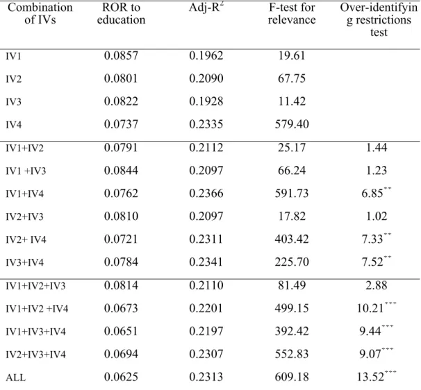
shown in Table 5.

Table 5. Estimated rates of return to education for various combinations of IVs Combination

of IVs education ROR to Adj-R

2 _{F-test for}

relevance Over-identifying restrictions test IV1 0.0857 0.1962 19.61 IV2 0.0801 0.2090 67.75 IV3 0.0822 0.1928 11.42 IV4 0.0737 0.2335 579.40 IV1+IV2 0.0791 0.2112 25.17 1.44 IV1 +IV3 0.0844 0.2097 66.24 1.23 IV1+IV4 0.0762 0.2366 591.73 6.85** IV2+IV3 0.0810 0.2097 17.82 1.02 IV2+ IV4 0.0721 0.2311 403.42 7.33** IV3+IV4 0.0784 0.2341 225.70 7.52** IV1+IV2+IV3 0.0814 0.2110 81.49 2.88 IV1+IV2 +IV4 0.0673 0.2201 499.15 10.21*** IV1+IV3+IV4 0.0651 0.2197 392.42 9.44*** IV2+IV3+IV4 0.0694 0.2307 552.83 9.07*** ALL 0.0625 0.2313 609.18 13.52***

Notes: 1. IV1 for compulsory educational policy; IV2 for residence area; IV3 for number of siblings; and IV4 for father’s education.

2. If F-statistic is smaller than 10, it implies that the selected IV has no explanatory power and will cause an estimation bias for return to education.

3. Null hypothesis of over-identifying restriction is that all the including instrumental variables are jointly exogenous.

4. *, **, and *** represent the statistical significance levels at 90%, 95%, and 99%, respectively.

From Table 5, we find that the inclusion of more IVs will reduce the estimated rate

of return to education, as the result from one single IV represents one particular

demographic subgroup. The inclusion of further IVs will increase the explanatory

return to education will conceptually approach the real average marginal rate of return

to education at the second stage wage regression.

However, the two conditions of instrument relevance and exogeneity still need to

be satisfied as valid instruments. Moreover, the criterion for the most effective valid

instrument among the IVs is the one that provides the minimum mean square error

(MSE) for the estimation of rate of return to education at the second stage wage

regression. From Table 5, we find that any single instrumental variable satisfies the

instrument relevance condition; however, every IV combination that includes the

father’s education (IV4) will reject the null hypothesis of the over-identifying

restrictions test, suggesting that the father’s education fails to satisfy the instrument

exogeneity condition and thus is not a valid instrument for education. Among all the

IV combinations, the combination of compulsory education policy (IV1) and

residence area (IV2) not only satisfies both the relevance and exogeneity conditions

but also has the lowest MSE value. Thus, the combination of IV1 and IV2 is the most

effective valid instrument for education variable. Table 6 shows the estimated rates of

return to education for both males and females using IV1+IV2 as the instrument for

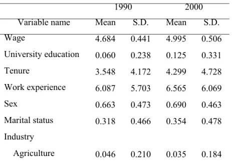
Table 6. Estimated rates of return to education for males and females

OLS IV1+IV2

Explanatory

variable Male Female Male Female

Years of education 0.0531*** _0.0465*** _0.0771*** _0.0621*** _0.0572*** _0.0480*** _0.1407*** _0.1009*** (21.21) (18.66) (26.96) (21.01) (7.33) (7.05) (13.07) (11.25) Tenure 0.0471*** _0.0401*** _0.0566*** _0.0551*** _0.0410*** _0.0312*** _0.0363*** _0.0302*** (16.88) (13.28) (11.32) (10.98) (13.65) (11.95) (4.11) (4.95) Tenure2 _-0.0017** * -0.0015 ** * -0.0015 ** * -0.0017 ** * -0.0015 ** * -0.0011 ** * 0.0005 -0.0005 (-14.46) (-11.78) (-4.66) (-3.87) (-12.62) (-10.13) (1.12) (-0.77) Work experience 0.0209*** _0.0178*** _0.0266*** _0.0243*** _{0.0015 -0.0014 -0.0069}* _0.0054 (9.13) (7.42) (8.98) (8.22) (0.77) (-0.98) (-1.66) (0.77) Work experience2 -0.0003 ** * -0.0003** -0.0005 ** * -0.0004 ** * 0.0002** 0.0002** 0.0005*** 0.0002 (-4.11) (-3.07) (-3.16) (-2.96) (2.66) (2.17) (2.43) (0.98) Marital status 0.0868*** _{0.0092 0.1212}*** _0.0081 (8.21) (0.29) (9.95) (0.44) Industry Agriculture -0.3672** * -0.0941 -0.4166 ** * -0.0883 (-11.45) (-0.74) (-15.11) (-0.76) Manufacturing _-0.0086 -0.0642** * -0.0583 ** * -0.1744 ** * (-0.67) (-2.71) (-3.07) (-9.12) Water, electricity, fuel, and coal 0.1862** (3.23) 0.1177 (0.41) 0.1566** (1.82) 0.2256 (0.17) Construction 0.1544*** _{0.0011 0.0849}*** _0.0064 (8.03) (0.21) (3.93) (0.08) Transportation, storage, and communications 0.0569 *** (2.66) 0.0476 (1.33) 0.0432 (1.50) 0.0481 (0.87)

Finance, insurance, and real estate 0.1369*** (3.98) 0.0612** (2.78) 0.1897*** (5.93) 0.0668*** (2.62) Personal and public services -0.0054 (0.56) -0.0671** * (-3.34) -0.0107 (-0.43) -0.0763** * (-3.77) Firm size 10-49 persons 0.0393** _0.0887*** _0.0497*** _0.1043*** (2.91) (4.07) (3.21) (6.44) 50-99 persons -0.0072 0.1487*** _0.0526* _0.2284*** (-0.43) (6.01) (1.79) (9.93) 100-499 persons 0.0104 0.1266*** _0.0796*** _0.2088*** (0.66) (5.88) (2.99) (8.12) 500 persons and above 0.0388 (1.12) 0.1702*** (6.33) 0.1203*** (4.41) 0.2227*** (6.77) Public sector 0.0533** _0.2875*** _0.1621*** _0.3605*** (2.66) (10.43) (7.12) (14.94) Correction term λ -0.5321 ** * -0.4817 ** * 0.3144*** 0.2907*** -1.4532 ** * -1.3783 ** * 0.7328*** 0.5568*** (-20.62) (-19.11) (11.25) (9.69) (-9.93) (-8.45) (7.76) (6.94) Constant 3.8622*** _3.9328*** _3.2918*** _3.1084*** _4.0221*** _3.9029*** _2.6891*** _3.1209*** (111.73) (101.45) (78.66) (69.33) (43.45) (40.19) (21.12) (26.43) Observations 4769 4769 2424 2424 4769 4769 2424 2424 Adj-R2 _{0.1483 0.2203 0.2750 0.3164 0.1046 0.1715 0.1302 0.2401}

Notes: See Notes in Table 3.

Results from Table 6 suggest that the estimated rate of return to education is

higher for females than for males for both the OLS and IV methods, and that the

estimated return to education is higher for the IV method than for the OLS method for

method. For the parsimonious formation of wage equation with only education, tenure,

and work experience as the explanatory variables, the estimated rate of return to

education is 5.31% for males and 7.71% for females by the OLS, and that of the IV

method is 5.72% for males and 14.07% for females.27 _{Including additional}

explanatory variables of marital status, affiliated industry, and firm size, the estimated

rate of return to education is 4.65% for males and 6.21% for females by the OLS, and

that of the IV method is 4.80% for males and 10.09% for females. These results imply

that the downward bias by OLS estimation is greater for females than for males, as

females are likely to be underinvested in or discriminated against in education due to

family background factors. Thus, for those whose educational choice is critically

influenced by family factors, such as females, the IV method will mitigate the

endogenous downward bias and provide a better estimate for their marginal rates of

return to education.

IV. Conclusion

Conventional OLS estimation of rate of return to education by the Mincerian

wage equation has its statistical simplicity in empirical studies, provided that the

assumption is not true, as is indeed the case in educational choice, the endogeneity of

the education variable will cause the estimated rate of return to education to be biased

downward by the OLS method. To solve for the endogeneity problem, this paper uses

the IV method to estimate rate of return to education using data from the 1990 Taiwan

Manpower Utilization Survey. Instrumental variables include the nine-year

compulsory education policy, residence area, number of siblings, and father’s

education. Except the father’s education, the other three IVs satisfy both the

instrument relevance and exogeneity conditions.

The results show that the estimated rate of return to education is higher for the

IV method than for the OLS method. Among them, the highest estimated rate of

return to education (8.57%) is for the instrument of compulsory education policy,

implying that a comprehensive institutional change such as a nationwide compulsory

educational policy significantly reduces the marginal cost of education for the people,

especially those who are subject to family credit constraints. Thus, the impact on

education is greater for the compulsory educational policy than for residence area or

family factor.

As there is more than one instrument, any combination of IVs can be a valid

stage wage regression as the most effective valid instrument. The result shows that the

combination of compulsory education policy (IV1) and residence area (IV2) is the

most efficient valid instrument, which may give a better estimation for the rate of

return to education. Using this instrument, we further estimate rates of return to

education for both males and females, finding that the estimated rate of return to

education is 5.72% for males and 14.09% for females, which is higher than that found

by OLS, especially in the female group. As females are likely to be underinvested or

discriminated against in education due to family credit constraints, this paper shows

that the downward bias will become more serious for females than for males through

References

Angrist, J. D. and A. B. Krueger (1991), “Does Compulsory Schooling Attendance After Schooling and Earning?” Quarterly Journal of Economics, 106(4), 979-1014.

Arcand, J. L., B. D’hombres and P. Gyselinck (2004), “Instrument Choice and the Returns to Education: New Evidence from Vietnam,” Economics Working Paper Archive at WUSTL, 0510011.

Barro, R. J., and X. Sala-i-Martin (1995), Economic Growth, Cambridge, MA: MIT Press.

Bound J., Jaeger D. A. and R. Baker (1995), “Problems with Instrumental Variables Estimation When the Correlation between the Instruments and the Endogenous Explanatory Variable is Weak,” Journal of the American Statistical Association, 90, 443-450.

Card, D. (1999), “The Causal Effect of Education on Earnings,” In Ashenfelter, O. and D. Card, (eds) Handbook of Labor Economics, Vol. 3A, Amsterdam: Elsevier.

Card, D. (2001), “Estimating the Return to Schooling: Progress on Some Persistent Econometric Problems,” Econometrica, 69(5), 1127-1160.

Chuang, Y. C. (1999), “The Role of Human Capital in Economic Development: Evidence from Taiwan,” Asian Economic Journal, 13, 117-144.

Chuang, Y. C. (2000), “Human Capital, Exports, and Economic Growth: A Causality Analysis for Taiwan, 1952-1995,” Review of International Economics, 8, 712-720.

Chuang, Y. C. and C. Y. Chao (2001), “Educational Choice, Wage Determination, and Rates of Return to Education in Taiwan,” International Advances in Economic Research, 7, 479-504.

Cruz, L. M. and M. J. Moreira (2005), “On the Validity of Econometric Techniques with Weak Instruments: Inference on Returns to Education Using Compulsory School Attendance Laws,” Journal of Human Resources, 40 (2), 393–410.

Davidson R. and J. G. MacKinnon (2003), Econometric Theory and Methods, Oxford, UK: Oxford University Press.

Donald, S. and W. Newey (2001), “Choosing the Number of Instruments,” Econometrica, 69(5), 1161-1191.

Duflo, E. (1999), “Schooling and Labor Market Consequences of Schooling in Indonesia: Evidence from an Unusual Policy Experiment,” Mimeo, Department of Economics, MIT

Durbin, J. (1954), “Errors in Variables,” International Statistical Review, 22, 23-32.

Gindling, T. H., M. Goldfarb and C.C. Chang (1995), “Changing Return to Education in Taiwan,” World Development, 23(2), 343-356.

Griliches, Z. (1977), “Estimating the Return to Schooling: Some Econometric Problems,” Econometrica, 45(1), 1-22.

Gurgand, M. (2003), “Farmer Education and the Weather: Evidence from Taiwan (1976–1992),” Journal of Development Economics, 71, 51–70.

Hansen L. P. (1982), “Large Sample Properties of Generalized Method of Moments Estimators,” Econometrica, 45, 1-22.

Harmon, C. and I. Walker (1995). “Estimates of the Economic Return to Schooling for the UK,” American Economic Review, 85, 1279-1286.

Hausman J. (1978), “Specification Test in Econometrics,” Econometrica, 46(3), 262-280.

Haveman, R. and B. Wolfe (1995), “The Determinants of Children’s Attainments: A Review of Methods and Findings,” Journal of Economic Literature, 33, 1829-1878.

Heckman J. J. (1976), “The Common Structure of Statistical Models of Truncation, Sample Selection, and Limited Dependent Variables and a Simple Estimator for Such Models” Annals of Economic and Social Measurement,5, 475-492.

Heckman, J. J., R. J. Lalonde, and J. A. Smith (1999), “The Economics and Econometrics of Active Labor Market Programs,” In Ashenfelter, O. and D. Card, (eds) Handbook of Labor Economics, Vol. 3A, Amsterdam: Elsevier.

Heckman, J. J., L. J. Lochner, and P. E. Todd (2003), “Fifty Teatrs of Mincer Earnings Regressions,” Working Paper 9732, National Bureau of Economic Research, Cambridge, MA.

Heckman J. J. and E. Vytlacil (1999), “Local Instrumental Variable and Latent Variable Models for Identifying and Bounding Treatment Effects,” Proceedings of the National Academy of Sciences, 96, 4730-4734.

Johnston, J. and J. Dinardo (1997), Econometrics Methods, 4th edition, Macraw-Hill.

Lin, T. C. (2004), “The Role of Higher Education in Economic Development: An Empirical Study of Taiwan Case,” Journal of Asian Economics, 15, 355–371

Mincer, J. (1974), Schooling Experience and Earning, New York: Columbia University Press.

Moretti, E. (2004), “Estimating the Social Return to Higher Education: Evidence from Longitudinal and Repeated Cross-Sectional Data,” Journal of Econometrics, 121(1-2), 175-212.

Patrinos, H. and C. Sakellariou (2005), “Schooling and Labor Market Impacts of a Natural Policy Experiment,” Labour, 19(4), 705-719.

Psacharopouls, G. (1985), “Return to Education: A Further International Update and Implications,” Journal of Human Resources, 20(4), 583-604.

Sakellariou C. (2006), “Education Policy Reform, Local Average Treatment Effect and Returns to Schooling from Instrumental Variables in the Philippines,” Applied Economics, 38, 473-481.

Sargen J. (1958), “The Estimation of Economic Relationships Using Instrumental Variables,” Econometrica, 26(3), 393-415.

Spohr, C.A. (2003), “Formal Schooling and Workforce Participation in a Rapidly Developing Economy: evidence from ‘Compulsory’ Junior High School in Taiwan,” Journal of Development Economics, 70, 291–327.

Steiger D. and J. H. Stock (1997), “Instrumental Variables Regression with Weak Instruments,” Econometrica, 65(3), 557-586.

Trostel P., I. Walker and P. Woolley (2002), “Estimates of the Economic Return to Schooling for 28 Countries,” Labour Economics, 9(1), 1-16.

Wu, D. (1973), “Alternative Tests of Independence Between Stochastic Regressors and Disturbances,” Econometrica, 41, 733-750.

Wu, H. Y. (2003), “An Economic Evaluation of Taiwan’s Educational Development: 1978-2001,” Taiwan’s Economic Forecast and Policy, 33(2), 97-130. (in Chinese)

Heterogeneity, Comparative Advantage, and Return to Education:

The Case of Taiwan

Abstract

By considering heterogeneity in abilities and self-selection in educational choice, this paper adopts the heterogeneous human capital model to estimate rate of return to university education using data from the 1990 and 2000 Taiwan’s Manpower Utilization Surveys. The Taiwan empirical study shows that significant heterogeneous return to education does exist, and that the educational choice was made according to the principle of comparative advantage. The estimated rates of return for attaining university were 19% and 15%, much higher than the average rate of return of 11.55 and 6.6%, for 1990 and 2000, respectively. The declining trend of return to university education may have been caused by the rapid expansion of the number of colleges and universities and the increasing supply of college graduates in the 1990s.

Keywords: Heterogeneous human capital; Sorting gain; Selection bias; Return to education; Marginal treatment effect; Average treatment effect

Heterogeneity, Comparative Advantage, and Return to Education:

The Case of Taiwan

I. Introduction

According to human capital theory, people invest in education to accumulate

human capital, enhance personal productivity, and in return receive higher life-cycle

earnings profiles.28 _{The economic return to education not only affects the individual’s}

educational choice and hence his life-cycle earnings but also influences the labor

quality of the whole society, an important factor for the aggregate performance of the

economy and for the planning of government educational policy. Thus, the estimation

of the return to education has become one of the most essential issues in modern labor

economics.

What is the “true” rate of return to education? Education is a form of human

capital investment and accumulation; however, the formulation and identification of

human capital may be quite diverse and usually result in different estimation methods

for the rate of return to education. There are two viewpoints on the formulation of

human capital. One is, human capital is homogenous, and people may choose to have

different units of human capital through investment like education and on-the-job

training, ending up with different stocks of human capital by themselves.29 Following

28 _{See, for example, Card (1999) for a complete theoretical and empirical survey on the relationship}

this line of view, researchers use the common coefficient model to estimate the return

to education from the Mincerian wage equation and emphasize the problems of ability

bias and measurement error. The OLS or instrumental variables methods are usually

employed. Another opinion, as in Roy (1951),Willis and Rosen (1979), and Willis

(1986), views human capitals as heterogeneous multidimensional attributes, and

people choose their educational attainment based on the comparative advantage of

their different attributes of abilities. In the case of heterogeneous human capital, the

random coefficient model is usually adopted to estimate the returns on education.

A major problem in the estimation is that education is an investment decision,

and thus the schooling variable is endogenous, which is against the basic exogeneity

assumption of explanatory variables in OLS estimation. Moreover, education is a

self-selection process. In the real world, the data that we observe are results after

selection, and thus not a random sample. For example, it is not possible to find the

wages for those who have received college and university education if instead they

enter the labor market right after they graduate from high school. As a result, the error

term in the regression equation is truncated, and it renders selection bias for the

estimator. If human capital is heterogeneous, as in the Roy model, then heterogeneity

in abilities will reinforce the process of self-selection and thus exacerbate the effect of

selection bias.

Following Roy’s (1951) heterogeneous human capital model and Bjorklund and

Moffitt’s (1987) concept of marginal treatment effect (MTE), Heckman and Vytlacil

(1999, 2000), and Carneiro, Heckman, and Vytlacil (2001) develop a model to

estimate the return to education with heterogeneous human capital.30 _{The main}

features of the model are that the estimation results can be used to test the hypothesis

of heterogeneous human capital and further estimate the average treatment effect

(ATE) and trace the selection bias.

For the past four decades, Taiwan, a small island of 36,000 kilometers with

limited natural resources, has achieved a so-called “economic miracle,” with an

average annual economic growth rate of 8.45% between 1960 and 2000. The

investment in education has expanded greatly in Taiwan. The average years of

education for employed workers in Taiwan have increased tremendously from 7.18

years in 1978 to 11.03 years in 2006, while for the same period, the per capita income

rose from US$1,461 to US$14,455, a roughly ten-fold increase. Thus, the estimation

of the economic return from education is especially relevant. Using data from the

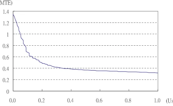
30 _{The marginal treatment effect is the average return for those who are at the critical status of}

1990 and 2000 Taiwan’s Manpower Utilization Surveys, this paper adopts the

heterogeneous human capital model to estimate the rate of return to college and

university education in Taiwan and compares the estimation results with that from the

conventional OLS or IV estimation methods.

This paper is organized as follows. Section 2 lays out the theoretical framework

and empirical method for the heterogeneous human capital model. Section 3 contains

data description and analysis. Section 4 presents estimation results of Taiwan’s

2. An empirical model for heterogeneous human capital

Heterogeneous return on education

In the conventional Mincerian earning equation with the assumption of

homogeneous human capital, the common coefficient model can be expressed as

i i i i S X U Y =β +γ + ln , (1)

where i is an index for the individual; ln is the worker’s average hourly real Y_i

wage in logarithmic form; S_i is years of schooling; X_i represents other variables

that influence an individual’s real wage, including tenure, work experience, sex,

marital status, affiliated industry, and firm size; and U_i is random error. The

coefficient β is the rate of return to an additional year of education.

Due to ability bias and selection bias, OLS estimation for equation (1) will result

in the estimation of the average marginal rate of return to education being biased. A

useful tool to deal with the problem is the instrumental variable method, that is, to

find a set of relevant instruments which is correlated with the schooling variable but

uncorrelated with the real wage or error term; see, for example, Angrist and

Krueger(1991), Trostel, Walker, and Woolley(2002), Patrinos and Sakellariou (2005),