基於EEMD之倒傳遞類神經網路方法對用電量及黃金價格之預測 - 政大學術集成

全文

(1)國立政治大學理學院應用物理研究所碩士論文 Graduate Institute of Applied Physics, College of Science National ChengChi University Master Thesis. 基於 EEMD 之倒傳遞類神經網路方法對用電量及治. 政. 大. 立黃金價格之預測. ‧ 國. 學. Forecasting electricity consumption as well as gold price. ‧. by using an EEMD-based Back-propagation Neural. Nat. n. al. er. io. sit. y. Network Learning Paradigm. Ch. engchi. i Un. v. 蔡羽青 Tsai Yu Ching 指導教授：蕭又新博士 Advisor：Shiau Yuo Hsien. 中華民國一○○年九月 September, 2011.

(2) 摘. 要. 本研究主要應用基於總體經驗模態分解法(EEMD)之倒傳遞類神經網路(BPNN) 預測兩種不同的非線性時間序列數據，包括政大逐時用電量以及逐日歷史黃金價格。透過 EEMD，這兩種資料會分別被拆解為數條具有不同物理意義的本徵模態函數(IMF)，而這讓我們可以將這些 IMF 視為各種影響資料的重要因子，並且可將拆解過後的 IMF 放入倒傳遞類神經網路中做訓練。另外在本文中，我們也採用移動視窗法作為預測過程中的策略，另外也應用. 政治大. 內插法和外插法於逐時用電量的預測。內插法主要是用於補點以及讓我們的數據. 立. 變平滑，外插法則可以在某個範圍內準確預測後續的趨勢，此兩種方法皆對提升. ‧ 國. 學. 預測準確度占有重要的影響。. 利用本文的方法，可在預測的結果上得到不錯的準確性，但為了進一步提升. ‧. 精確度，我們利用多次預測的結果加總平均，然後和只做一次預測的結果比較，. y. Nat. n. al. Ch. engchi. er. io. 練過程中其目標為尋找最小誤差函數的關係所致。. sit. 結果發現多次加總平均後的精確度的確大幅提升，這是因為倒傳遞類神經網路訓. i Un. v. 關鍵字：總體經驗模態分解法、倒傳遞類神經網路、用電量預測、黃金價格預測、超短時間負荷預測. 1.

(3) Abstract. In this paper, we applied the Ensemble Empirical Mode Decomposition (EEMD) based Back-propagation Neural Network (BPNN) learning paradigm to two different topics for forecasting: the hourly electricity consumption in NCCU and the historical daily gold price. The two data series are both non-linear and non-stationary. By applying EEMD, they were decomposed into a finite, small number of meaningful Intrinsic Mode Functions (IMFs). Depending on the physical meaning of IMFs, they can be regarded as important variables which are input into BPNN for training.. 政治大. We also use moving-window method in the prediction process. In addition, cubic. 立. spline interpolation as well as extrapolation as our strategy is applied to electricity. ‧ 國. 學. consumption forecasting, these two methods are used for smoothing the data and. ‧. finding local trend to improve accuracy of results.. The prediction results using our methods and strategy resulted in good accuracy.. y. Nat. er. io. sit. However, for further accuracy, we used the ensemble average method, and compared the results with the data produced without applying the ensemble average method.. n. al. Ch. i Un. v. By using the ensemble average, the outcome was more precise with a smaller error,. engchi. it results from the procedure of finding minimum error function in the BPNN training.. Keywords: Ensemble Empirical Mode Decomposition, Back-propagation Neural Network, electricity consumption forecasting, gold price forecasting, very-short term load forecasting. 2.

(4) Contents 1. Introduction ................................................................................................................ 7 2. Methodology ............................................................................................................ 12 2.1 Empirical mode decomposition ..................................................................... 12 2.2 Ensemble EMD ............................................................................................ 15 2.3 Artificial neural networks ............................................................................ 17 2.4 Cubic spline interpolation and extrapolation ............................................... 23 2.5 EEMD-based neural network learning paradigm ........................................ 24. 政治大. 3. Forecasting experiments ......................................................................................................... 26. 立. ‧ 國. 學. 3.1 Data description ............................................................................................. 26 3.1.1. Electricity load data from NCCU ................................................................. 26. ‧. 3.1.2. Gold price daily data ..................................................................................... 27. sit. y. Nat. 3.2 Experiment design ....................................................................................... 29. n. al. er. io. 3.3 Statistical measures ...................................................................................... 33. i Un. v. 4. Results and discussion ............................................................................................................. 37. Ch. engchi. 4.1 Benchmark study............................................................................................................. 37 4.2 The meaning of IMFs .................................................................................................... 40 4.3 Forecasting performance ............................................................................................ 45 4.4 Performance of ensemble average ........................................................................... 48 4.4.1. Electricity load data from NCCU ................................................................. 48 4.4.2. Gold price daily data ..................................................................................... 53 5. Conclusion and outlook ........................................................................................................... 56 APPENDIX .................................................................................................................. 57 Reference ................................................................................................................... 59 3.

(5) Tables Table 4.1 Comparison between different input data length for forecasting of 2011 gold price .................................................................................................................... 37 Table 4.2 Comparison between different input data length for forecasting of June 6, 2008 of GCB10 ........................................................................................................... 39 Table 4.3 Measures of IMFs for General Building of NCCU from May 30 to June 5, 2008............................................................................................................................. 42. 政治大. Table 4.4 Measures of IMFs for gold price daily data from 2007 to 2010 ................. 44. 立. Table 4.5 Forecasted hourly load compared with actual load for June 6, 2008 of. ‧ 國. 學. GCB10 ........................................................................................................................ 45. ‧. Table 4.6 The performance comparison between different ensemble average levels 52. y. Nat. er. io. sit. Table A.1 The mean error and collation of points over 5% of GCB10 from May 12 to June 6, 2008 except for weekends…………………………………………………...58. n. al. Ch. engchi. i Un. v. 4.

(6) Figures Figure 2.1 The flowchart of EMD .............................................................................. 14 Figure 2.2 Diagram to illustrate the procedure of Ensemble EMD ............................ 16 Figure 2.3 Simple structure chart of three-layers neural network .............................. 17 Figure 2.4 The structure chart of complete four-layer BPNN .................................... 21 Figure 2.5 The flowchart of training progress of BPNN ............................................ 22 Figure 2.6 Simple illustration of EEMD to form the inputs of neural network .......... 24 Figure 3.1 Hourly electricity load curve of GCB10 from 2008.5.5 to 2008.6.6......... 27 Figure 3.2 Monthly gold price and significant world events from Jan. 1968 to. 治政 Nov.2010..................................................................................................................... 28 大立 Figure 3.3 The interpolation method .......................................................................... 29 ‧ 國. 學. Figure 3.4 Create a new data series by interpolation and extrapolation ..................... 30. ‧. Figure 3.5 Training Network by Moving Window Process ........................................ 32. sit. y. Nat. Figure 4.1 The IMFs for General Building of NCCU from May 30 to June 5, 2008 . 41. io. al. er. Figure 4.2 The IMFs of historical gold price daily data from 2007 to 2010 .............. 44 Figure 4.3 Forecasting performance for June 6, 2008 of GCB10 ............................... 46. n. iv n C Figure 4.4 Forecasting performancehof every hour forU e n g c h i June 6, 2008 of GCB10…….47 Figure 4.5 The performance of correlation between forecasted and actual hourly. data...............................................................................................................................47 Figure 4.6 A diagrammatic sketch of the BPNN error function……………………..48 Figure 4.7 Forecasting performance for May 22, 2008 of GCB10, without ensemble average ........................................................................................................................ 50 Figure 4.8 Forecasting performance for May 22, 2008 of GCB10, with three times ensemble average………………………………….....................................................51 Figure 4.9 Forecasting performance for May 22, 2008 of GCB10, with five times ensemble average…………………………………………………………………….51 5.

(7) Figure 4.10 Forecasting performance for 2011 gold price daily data, without ensemble average ........................................................................................................................ 54 Figure 4.11 The performance of correlation between forecasted and actual daily data for gold price daily data without ensemble average……………………………….....54 Figure 4.12 Forecasting performance for 2011 gold price daily data, with five times ensemble average…………………………………………………………………….55 Figure 4.13 The performance of correlation between forecasted and actual daily data for gold price daily data with five times ensemble average..……………...…………55 Figure A.1 Statistics of points over 5% of GCB10 from May 12 to June 6, 2008. 治政 except for weekends..……………...……………………...………………………….57 大立 ‧. ‧ 國. 學. n. er. io. sit. y. Nat. al. Ch. engchi. i Un. v. 6.

(8) 1. Introduction Empirical Mode Decomposition (EMD), first introduced by Huang et al. (1998) was developed for dealing with nonlinear and non-stationary data. The method is empirical, intuitive, direct and adaptive. By using EMD, the time-series data is decomposed into several intrinsic modes which are nearly periodic and independent with each other. The intrinsic modes may have its own physical meaning based on local characteristic time scale. For instance, if an intrinsic mode is periodic with a time scale of one month, it can be recognized as the monthly component. Similarly,. 治政 Generally, complex time-series data is often mixed 大 up with many different signal 立 an intrinsic mode with scale of three months means the seasonal component.. sources thus difficult to understand their meaning. But, through the EMD. ‧ 國. 學. decomposition method we can divide them into several meaningful intrinsic modes,. ‧. allowing us to closely analyze their characteristics.. sit. y. Nat. EMD has been successfully applied in different fields such as ocean waves. io. al. er. (Hwang et al., 2003), earthquake engineering (RR Zhang et al., 2003), wind engineering (Li and Wu, 2007), biomedical engineering (Liang et al., 2005) and. n. iv n C structured health monitoring (R Yan, above applications are all related to h e2006). n g The chi U natural science and engineering. However, in the recent years, there have been more and more applications in social sciences. For example, financial time series analysis (Huang et al., 2003b), transport geography (MC Chen, 2010), disease transmission (Cummings et al., 2004), as well as combined with artificial neural networks (ANNs) to forecast crude oil price (Lean Yu et al., 2008). In addition to the EMD originally developed, there is an improved EMD, known as Ensemble EMD (EEMD, Wu and Huang, 2009), which was proposed to solve the mode mixing problem of EMD. In this study, we first applied the EEMD method and 7.

(9) then combined it with ANNs to electricity consumption forecasting and gold price forecasting. Electricity consumption forecasting (i.e. load forecasting), is commonly classified into four categories: long-term load forecasting, medium-term load forecasting, short-term load forecasting and very short-term load forecasting. Long-term load forecasting (5, 10 and 20 years ahead) is used for system planning, scheduling construction of new generation capacity and the purchasing of generation units (Jia et al., 2001). Medium-term load forecasting (a few months to 5 years ahead) is applied to maintenance scheduling, coordination of load dispatching and the setting of prices. 治政 (Jia et al., 2001). Short-term load forecasting (hourly forecasting from one day to one 大立 week ahead) is usually used for optimal generator unit commitment, fuel scheduling, ‧ 國. 學. hydro-thermal co-ordination, economic dispatch, generator maintenance scheduling,. ‧. the buying and selling of power and security analysis. Very short term load. sit. y. Nat. forecasting (few minutes to an hour ahead in the future) is often used for security. io. al. er. assessments and economic dispatching, real-time control and real-time security. n. evaluation (Jia et al., 2001). In this study we focused on very short-term load. ni forecasting and forecast load of C onehhour ahead. U engchi. v. Surprisingly, there has been very little research on very short-term load forecasting. Yang et al. (2005) used a method based on the chaotic dynamics reconstruction technique and fuzzy logic theory on the load data of Shandong Heze Electric Utility, (China). Their results demonstrated that the proposed approach could calculate 15 minutes ahead load forecasting with accurate results. James W. Taylor (2008) used minute-by-minute British electricity demand observations to evaluate different forecasting methods, including ARIMA modeling and Holt-Winters' exponential smoothing method for prediction between 10 and 30 minutes ahead. Liu et al. (1996) applied the fuzzy logic method and ANNs to the previous 30 minute-by-minute 8.

(10) observations as input for the online forecasting process to show that the methods could outperform the simplistic non-seasonal AR model. Unlike the various aforementioned methods, we used the EEMD-based ANN algorithm for one hour ahead forecasting. ANNs are massively parallel and robust. They contain complicated architectures of interconnected processing elements. They can learn complex linear or non-linear input-output mappings between data sets of measurements and future demand values. Based on the features presented in the data they can be designed adaptively for learning and responding with high-speed computation. The ANNs have been applied to many areas especially when dealing with the issues of forecasting.. 立. 政治大. Hamid et al. (2004) applied ANNs to financial forecasting. Their goal was to. ‧ 國. 學. forecast the volatility of S&P 500 Index future prices, and compare volatility forecasts. ‧. from ANNs with the implied volatility from S&P 500 Index futures options using the. sit. y. Nat. Barone-Adesi and Whaley (BAW) model for pricing American options on futures.. io. er. Lean Yu et al. (2008) used an EMD-based neural network ensemble learning paradigm for world crude oil spot price forecasting. In Yu‘s study, West Texas. al. n. iv n C Intermediate (WTI) crude oil spot h price and Brent crude e n g c h i U oil spot price were used to test the effectiveness of the method. Their results showed that the EMD-based neural. network ensemble-learning model outperformed the other forecasting models in terms of criteria. Lean Yu et al. (2010) proposed an EMD-based multi-scale neural network learning paradigm to predict financial crisis events for early-warning purposes. They took the currency exchange rate series of the South Korean Won (KRW) and Thai Baht (THB) as training targets. Their tests showed that the EMD-based multi-scale neural network learning paradigm was superior to other classification methods and single-scale neural network learning paradigm when formulating currency crisis forecasting. Feng Ping et al. (2009) applied EMD-based ANNs to precipitation-runoff 9.

(11) forecasting. They took the annual precipitation series from 1956 to 2000 from the sub-water resource regions of upper Lanzhou, China as historical training data, and showed that the EMD could decompose the data into a multi-time scale sub-series for finding their local change rule. The results demonstrated that the EMD-based ANNs model presented higher accuracy than any other models. The ANNs are also widely used in short-term load forecasting. Ruey-Hsun Liang and Ching-Chi Cheng (2002) used an approach based on combing ANNs with the fuzzy system and applying it to data from the Taiwan Power Company. Nahi Kandil et al. (2006) applied multi-layered feed-forward ANNs by using data from. 治政 Hydro-Quebec databases for forecasting. They demonstrated ANNs‘ capabilities 大立 without using load history as an input, instead final temperatures were the only data ‧ 國. 學. considered in their load forecasting procedure. Mohsen Hayati and Yazdan Shirvany. ‧. (2007) used Multi-Layer Perceptron (MLP), a kind of architecture of ANNs, on data. sit. y. Nat. from a three year time period (2004-2006) from the Illam (Middle Eastern country,. io. Electric power system.. al. er. west of Iran) region, while G.A. Adepoju et al. (2007) applied ANNs to the Nigeria. n. iv n C Gold has been mined since ancient With recent growth in production, more h etimes. ngchi U. than a third of the world‘s gold that has ever been mined, in just the last thirty years. The consumption of gold differs by application type: industrial, dental technology, jewelry products and inventory. Jewelry consistently accounts for over two-thirds of the gold demand, but in markets with poorly developed financial systems or markets. experiencing crisis, gold is an attractive investment. The demand-supply equilibrium and inflation cause gold price to fluctuate. Gold is commonly a popular hedge instrument for investors against devaluation of the US dollar. In recent years as the value of US dollar has decreased relative to other major currencies, the price of gold 10.

(12) has experienced a secular increase. The dramatic rises in gold price since the start of 2009 may have resulted from investors looking to preserve their wealth. There have been several studies on gold price analysis: Baker and Tassel (1985) used regression results to support the theoretical analysis leading to the prediction. Akgiray, Booth, Hatem and Mustafa (1991) used the GARCH model to verify time decency of gold price. In comparison with statistical techniques, engineering- based systems, such as neural networks, make less restrictive assumptions on the underlying distribution. Mirmirani and Li (2004) used neural networks and genetic algorithm to analyze gold price. Shahriar Shafiee and ErkanTopal (2010) used long-term trend. 治政 reverting jump and dip diffusion model and took monthly 大 historical gold price data 立 from January 1968 to December 2008, to forecast gold price for the next ten years. ‧ 國. 學. Yen-Rue Chang (2011) used EEMD to decompose monthly gold price data into. ‧. several IMFs to observe their important properties. Following the work of Yen-Rue. y. sit. io. al. er. forecasting.. Nat. Chang (2011), we used the decomposed IMFs as input factors for gold price. This research aimed to forecast using EEMD-based ANN algorithm, more. n. iv n C specifically; we used a back-propagation network (BPNN) which is a kind of h e nneural gchi U ANN architecture. Our testing targets were electricity load data and gold price data. We performed one hour ahead load forecasting and gold price forecasting for 2011. Section 2 gives brief introduction to the basic concept of EEMD and BPNN. In section 3, we describe the subject data, and introduce our experiment strategy, and some important measures used. Experiment results and forecast performance are. discussed in Section 4, along with the results of improvement by ensemble average. In Section 5, we will present our conclusion and outlook.. 11.

(13) 2. Methodology 2.1. Empirical mode decomposition In the past, we usually used a spectral analysis method called the Fast-FourierTransform (FFT) to analyze time-series data; however FFT posed a few problems: If the nonlinear and non-stationary degrees of the time-series data were to increase, the results of the FFT would produce large sets of physically meaningless harmonics. Nowadays,. we. utilize. a. new. spectral. analysis. method. called. Hilbert-Huang-Transform (HHT). While the HHT can solve the problems with the FFT, it is still limited in that it can only be used for data which are symmetric in. 治政 relation to the local zero mean. We would thus need 大 to first use the empirical mode 立 decomposition (EMD) which was proposed by Huang et al. (1998) to decompose data ‧ 國. 學. into several intrinsic mode functions (IMFs). The IMFs are all symmetric in relation. ‧. to the local zero mean so that we can use HHT on them.. sit. y. Nat. The EMD is a data analysis method which can be used in dealing with non-linear. io. al. er. and non-stationary time series data. It assumes that all time series data can be decomposed into a sum of oscillatory functions known as IMFs. The IMFs, based on. n. iv n C the local characteristic scale by itself, to satisfy the two following conditions: h ehave ngchi U. (1) IMFs should have the same numbers of extrema (including maxima and minima) and zero-crossings, or differ at most by one; (2) At any point, the mean value of the envelope defined by local maxima and the envelope defined by local minima is zero, meaning the IMFs should be symmetric in relation to the local zero mean.. 12.

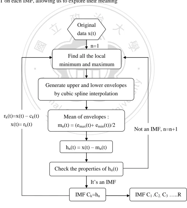
(14) We then pose the question, ‗how can we extract the IMFs from original data‘? We can use the following sifting process: (1) Identify all the local maxima and minima of the time series x(t) (2) Connect all the local maxima and minima by cubic spline interpolation to generate its upper and lower envelopes emax(t) and emin(t) (3) Calculate mean m(t) from upper and lower envelopes point-by-point as m1(t) = (emax(t)+ emin(t))/2 (4) Calculate the difference between the time series data x(t) and the mean value m1(t), than get h1(t) as :. h1(t) = x(t) - m1(t). 治政 (5) Check the properties of h (t): 大立 If h (t) doesn‘t satisfy the conditions of IMF, replace x(t) with h (t) and repeat 1. 1. 1. ‧ 國. 學. (1)-(4) until hk(t) satisfies the stopping criterion:. ‧ sit. y. Nat. io. er. A typical value for SD can be set between 0.2 and 0.3.. al. On the other hand, if h1(t) (or hk(t)) satisfies the conditions of IMF, then it should. n. iv n C be an IMF, and denote h1(t) (or hk(t)) IMF c1(t). Then we separate the IMF h easnthegfirst chi U c1(t) from x(t) to get the residue r1(t) : (6) Now. we. replace. x(t). with. x(t) - c1(t) = r1(t) r1(t). and. repeat. steps. (1)-(5). to. get. c2(t).c3(t).c4(t).c5(t)………..cn(t) and final residue rn(t).. The sifting process is stopped by any of the following predetermined criteria: either the component cn(t) or the residue rn(t) becomes so small that it is less than the predetermined value of the substantial consequence, or the residue rn(t) becomes a monotonic function from which no more IMFs can be extracted (Huang et al. 1998). At the end of the sifting process, the original time series can be expressed as 13.

(15) Where n is the number of IMFs, rn(t) is the final residue, also the trend of x(t), and ci(t) represents IMFs which are nearly orthogonal to each other. After the sifting process, the original data set is decomposed into these IMFs which represent high frequency to low frequency, and every IMF may have its own physical meaning. So we can regard the EMD as a filter to separate high to low frequency modes, and apply HHT on each IMF, allowing us to explore their meaning. data x(t). 學. ‧ 國. 立. 政Original治大 n=1. n. al. rk(t)=x(t) – ck(t) x(t)= rk(t). Ch. engchi. er. io. by cubic spline interpolation. sit. Nat. Generate upper and lower envelopes. y. ‧. Find all the local minimum and maximum. i Un. v. Mean of envelopes : mn(t) = (emax(t)+ emin(t))/2. Not an IMF, n=n+1. hn(t) = x(t) – mn(t). Check the properties of hn(t) It‘s an IMF IMF Ck=hn. IMF C1 .C2. C3 …..R. Figure 2.1 The flowchart of EMD 14.

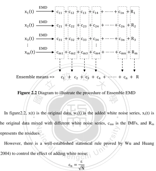
(16) 2.2. Ensemble EMD EMD has proved to be a useful data analysis method for extracting signals from nonlinear and non-stationary data. However, EMD still has its defects: when the original data is intermittent, a single IMF may consist of either signals of widely disparate scales, or a signal of similar scale belonging to different IMF components; this phenomenon is called ―mode mixing‖. When mode mixing occurs, an IMF may cease to have physical meaning by itself. Thus, EEMD was proposed by Wu and Huang (2004) for overcoming the problem. We know that all observed data are mixed with true time series and noise. Even if data is collected by separate observations with. 治政 different noise levels, the ensemble mean is close to the 大true time-series. This means 立 that we can extract the true meaningful signal from data by adding some white noise. ‧ 國. 學. Adding white noise could provide a uniformly distributed reference scale, and help. er. io. al. Add a white noise series to the original data.. sit. y. Nat. The simple procedure of EEMD is as follows: (1). ‧. EMD to overcome the mode mixing problem.. (3). Repeat the previous two steps iteratively, and add different white noise. n. (2). iv n C Decompose the data withhadded white noiseU e n g c h i into IMFs. each time, finally we obtain the ensemble means of corresponding IMFs of decompositions.. 15.

(17) EMD. EMD. EMD. EMD. Ensemble means =>. 立. 政治大. Figure 2.2 Diagram to illustrate the procedure of Ensemble EMD. ‧ 國. 學 ‧. In figure2.2, x(t) is the original data, wi(t) is the added white noise series, xi(t) is. sit. y. Nat. the original data mixed with different white noise series, cmn is the IMFs, and Rm. io. al. er. represents the residues.. n. However, there is a well-established statistical rule proved by Wu and Huang. C h white noise: U n i (2004) to control the effect of adding engchi. v. In this formula, N represents the number of ensemble members, of the added noise and. n. is the amplitude. is the final standard deviation of error defined as the. difference between the input signal and the corresponding IMFs. Empirically, the number of ensemble members N is always set to 100 and the. n is. always set to 0.1 or. 0.2. The procedure of adding white noise successfully makes signals of comparable scales to collate in one IMF, and then cancels itself out. Therefore, the EEMD, which. 16.

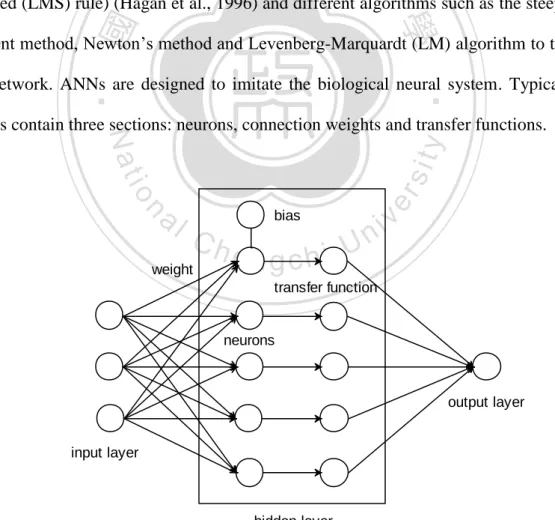
(18) can successfully reduce the chance of mode mixing, is a really good, substantial improvement over the original EMD.. 2.3. Artificial neural networks Artificial neural networks (ANNs), which have been widely used for data prediction in many application domains, are a kind of intelligent learning paradigm. They have been developed over the last 50 years, and the first, simplest model of ANNs which is called Perceptron was proposed by Frank Rosenblatt in 1957. Nowadays, the most popular model of ANNs is feed-forward back-propagation. 治政 neural network (BPNN). It adopts the Widrow-Hoff大 learning rule (i.e. least mean 立 squared (LMS) rule) (Hagan et al., 1996) and different algorithms such as the steepest ‧ 國. 學. descent method, Newton‘s method and Levenberg-Marquardt (LM) algorithm to train. ‧. the network. ANNs are designed to imitate the biological neural system. Typically,. n. al. Ch. weight. bias. engchi. er. io. sit. y. Nat. ANNs contain three sections: neurons, connection weights and transfer functions.. i Un. v. transfer function. neurons. output layer. input layer. hidden layer. Figure 2.3 Simple structure chart of three-layers neural network 17.

(19) The connection weights present the strength between neurons. A larger weight means the connection is stronger while a smaller weight presents a weaker link. The neurons process input signals overlap at the neuron and are sent to the transfer function for generating output value. The transfer functions are created to restrict the output value of ANNs. Because different kinds of ANNs are used in different ways, they need different transfer functions to generate different results. The feed-forward BPNN, which is the most popular model of ANNs for time-series data prediction, uses three kinds of transfer functions: log-sigmoid function, hyperbolic function and linear function. Log-sigmoid function and. 治政 hyperbolic function are often used in the hidden layer.大 The log-sigmoid function takes 立 an output value between 0 and 1 while the hyperbolic function takes an output value ‧ 國. 學. between 1 and -1. These two transfer functions are both differentiable so that the. ‧. training algorithms may work for the network, otherwise the linear function is usually. n. al. er. io. sit. y. Nat. put in the output layer. It can produce values of any number.. Ch. engchi. i Un. v. In this thesis, we used the feed-forward BPNN for modeling the decomposed IMFs and the residual component. In the BPNN, there is an important parameter called the ―mean square error function‖, which is a function of weights. Since our goal was to minimize the mean square error function, we had to adjust the connection weights iteratively by training the network. The mean square error function could be presented as: 18.

(20) where ai is the final output value, a function of weight. ti is the target value, and ei is the error between the values ai and ti. On the other hand, the input value of the mth layer‘s ith neuron is the nonlinear function of the output value of the (m-1)th layer‘s neurons:. 立. ‧ 國. 學. The function. 政治大. is the transfer function previously discussed. wijm is the weight. ‧. between the mth layer‘s ith neuron and (m-1)th layer‘s jth neuron, bim is the bias of. y. sit. io. n. al. er. value of mth layer.. Nat. mth layer‘s ith neuron, ajm-1 is the output value of (m-1)th layer, and aim is the output. i Un. v. In the history of BPNN, there have been several algorithms used to train the. Ch. engchi. network for adjusting the weight. Here we adopted the Levenberg-Marquardt (LM) algorithm, which combines the advantages of the steepest descent method and Newton‘s method:. 19.

(21) where Wm(k) is the matrix of weights in the mth layer after the kth adjustment. H(k) is called the ―Hessian matrix‖, which is the second derivative of the mean square error functions, and g(k) is the first derivative of F(w).. is the identity matrix, and. k. is. the control parameter. The control parameter. k changes. iteratively, set with a big value in the beginning.. Meanwhile, the LM algorithm will equal to the steepest descent method. The steepest descent method converges quickly when our result is still far from the optimal point, but as the result gets closer to the optimal point, the convergence speed gets slower, so the method costs much more times to find the optimal result.. 治政 The becomes a very small value in the later period 大 of training, meanwhile the 立 LM algorithm will become equal to Newton‘s method, which converges quickly when the result is approaching to the optimal result.. 學. ‧ 國. k. ‧. The significant reason why we chose BPNN as our prediction tool was that the. sit. y. Nat. BPNN is usually regarded as a ―universal approximator‖ (Hornik et al., 1989). Hornik. io. al. er. et al. found that a three-layer BPNN can approximate any continuous function arbitrarily well with an identity transfer function (i.e. linear transfer function) in the. n. iv n C output layer and logistic functions h (i.e. log-sigmoid function e n g c h i U and hyperbolic function) in the hidden layer. In practice, the neural networks with one and occasionally two hidden layers are. widely used and perform well. In this thesis, we utilized the four-layer feed-forward BPNN. Moreover, the number of neurons in the hidden layers were set to the same value as the IMFs or this value plus two, respectively, since the number of neurons in the hidden layer can range from one-half to two times (Mendelsohn, 1993) the sum of input and output numbers.. 20.

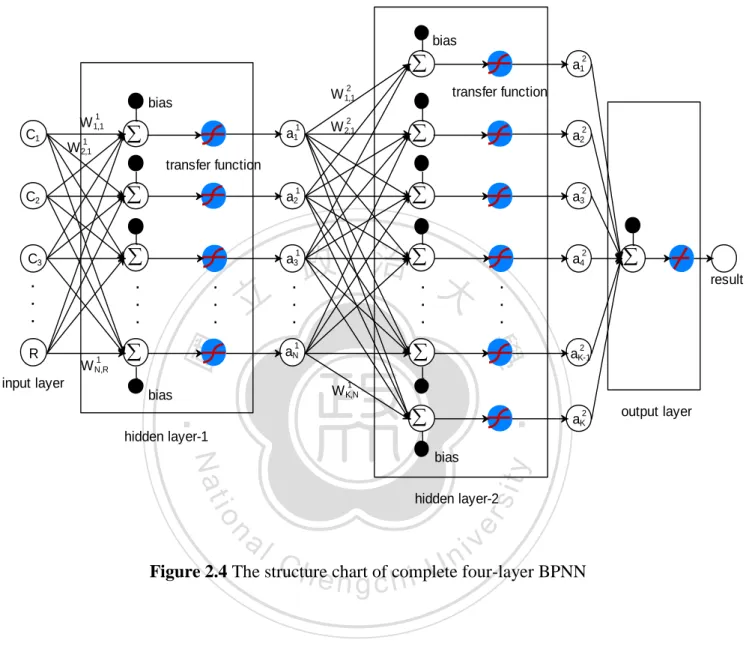
(22) The applied complete four-layer BPNN is shown as follows:. bias.  2. 1. C1. W 1,1 W. 1 2,1. transfer function. W 1,1. bias. . 1. a1. 2. W 2,1. 2. a1. . a2. . a3. 2. . a2. C3. . a3. . . .. . . .. . . .. . 立. . . .. 政治 大. 2. a4. . . .. . 1. aN.  result. . . . 2. aK-1. 1. W K,N. bias. ‧. . hidden layer-1. output layer. y. Nat. bias. 2. aK. io. sit. input layer. W. 1 N,R. 1. 2. hidden layer-2. al. er. R. 1. 學. C2. ‧ 國. transfer function. n. iv n C Figure 2.4 The structure h echart h i U four-layer BPNN n g ofc complete. 21.

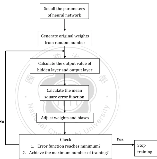
(23) Below is a flowchart of the BPNN learning progress which can help us to understand it more clearly.. Set all the parameters of neural network. Generate original weights from random number. 治政 Calculate the output value大 of 立 layer and output layer hidden ‧ 國. 學 y. n. al. Ch. engchi. sit. io. Adjust weights and biases. er. Nat. No. ‧. Calculate the mean square error function. i Un. v. Check 1. Error function reaches minimum? 2. Achieve the maximum number of training?. Yes Stop training. Figure 2.5 The flowchart of training progress of BPNN. 22.

(24) 2.4. Cubic spline interpolation and extrapolation Sometimes time-series data may be missing values. In the mathematical field of numerical analysis, interpolation is a method which is applied to fill the gaps of missing values. For generating those intermediate values, there are several interpolation methods, such as piecewise constant interpolation, linear interpolation, polynomial interpolation and cubic spline interpolation. In contrast with linear interpolation, cubic spline interpolation uses low-degree polynomials in each of the intervals, and makes the intervals of data points smooth. Extrapolation is a method which is used for forecasting outside of the known. 治政 values for a given range, but the results are often less 大meaningful. If applied to a 立 limited range of time-series data sets, extrapolation can extend data points, and find ‧ 國. 學. the variation tendency of the future of the time-series. Extrapolation uses the same. ‧. methods as interpolation. Linear extrapolation uses the last two data values to create a. sit. y. Nat. tangent line at the end of known data, extending it beyond the limit. However, it only. io. al. er. provides accurate results when used to extend the graph of an approximately linear function or not too far beyond the known data. Otherwise, cubic spline extrapolation,. n. iv n C which needs more than the two values h e nofgthec hendi ofUdata, can create a low-degree polynomial curve which is extended beyond the known data. It is suitable for data which has curve properties, or data which we have already applied the cubic spline interpolation to. In the use of the electricity load data of this study, the cubic spline interpolation method was applied to smooth the data points. Cubic spline extrapolation was employed to generate extra points to be included in our forecasting data before using the EEMD-based ANNs.. 23.

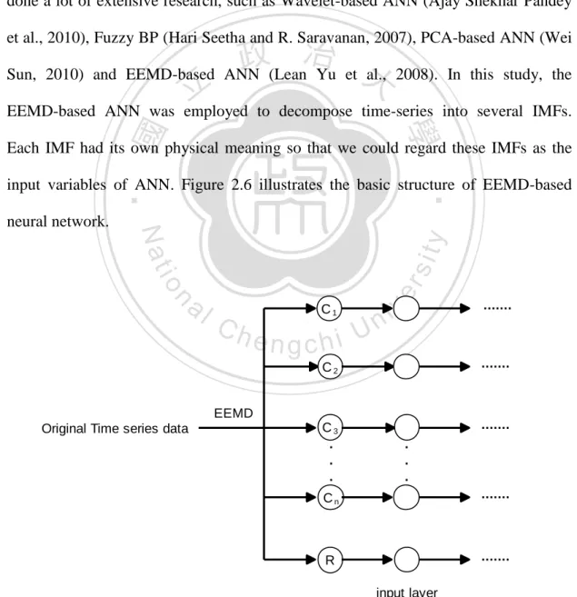
(25) 2.5. EEMD-based neural network learning paradigm Artificial neural networks, which have already been applied in many practical forecasting cases, still have a lot of room for improvement. A crucial challenge nowadays is to improve the performance of the forecasting of artificial neural networks. Some researchers advocate the cross-validation technique, but it may be inadequate when the problem is complex, due to the method being based on a single series representation for entire a training process. Consequently, many scholars have done a lot of extensive research, such as Wavelet-based ANN (Ajay Shekhar Pandey et al., 2010), Fuzzy BP (Hari Seetha and R. Saravanan, 2007), PCA-based ANN (Wei. 治政 Sun, 2010) and EEMD-based ANN (Lean Yu et 大 al., 2008). In this study, the 立 EEMD-based ANN was employed to decompose time-series into several IMFs. ‧ 國. 學. Each IMF had its own physical meaning so that we could regard these IMFs as the. n. al. er. io. sit. y. Nat. neural network.. ‧. input variables of ANN. Figure 2.6 illustrates the basic structure of EEMD-based. Ch. C1. engchi U. v ni. ........ C2 EEMD Original Time series data. C3 . . .. ........ ....... . . .. Cn. ........ R. ....... input layer. Figure 2.6 Simple illustration of EEMD to form the inputs of neural network 24.

(26) The EEMD-based neural network learning paradigm contains following steps: (1). Decompose the original data into IMFs and residual components using. EEMD. (2). Put IMFs as the input variables into the four-layer BPNN.. (3). The input data set and target data set are extracted from the decomposed IMFs and original data.. (4). In the program, the input values and target time-series data will be first manipulated to a range between 1 and -1, and then divided into training , testing and validation sets. When parameters are all fixed, the four-layer. optimal weights are found.. The other input data will input to the trained network, and the forecasting. ‧. (6). 學. ‧ 國. (5). 治政 BPNN structure will be created and start to train 大 the network. 立 In the network, the input data and target data will be compared and the. al. er. io. sit. y. Nat. data is generated. Then compare the forecasted data with real data.. To summarize, in this study we used EEMD to decompose the NCCU electricity. n. iv n C load data into several meaningful IMFs, combined extrapolation with BPNN h e nandg then chi U to forecast the electricity load of every hour. However the data used first underwent cubic spline interpolation. The forecasting results are shown in the next section.. 25.

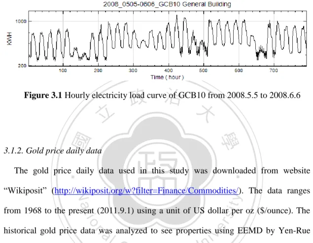
(27) 3. Forecasting experiments 3.1. Data description 3.1.1. Electricity load data from NCCU The used electricity load data in this study was obtained from Office of General Affairs of National Chengchi University (NCCU). In NCCU, the consumption of electricity mainly comes from ten regions, labeled as GCB1 to GCB10. Among these ten regions, only three are independent buildings while the remainders contain numerous different sources. The three important buildings which contribute a majority of the electricity consumption of NCCU are the Information Building. 治政 (GCB2), College of Commerce Building (GCB5) and大 General Building (GCB10). In 立 this thesis, we focused on these three buildings because the electricity is controlled ‧ 國. 學. more easily. Generally, the electricity consumption of NCCU gradually increases after. ‧. the anniversary celebrations, May 20, of every year. This is mainly due to the. io. al. er. air-conditioners and thus more consumption of electricity.. sit. y. Nat. approach of summer and increasing temperatures prompting more use of. The electricity load data possesses some important properties. To illustrate these. n. iv n C properties, we took the hourly datahfrom May 5, 2008 e n g c h i Uto June 6, 2008 of GCB10 for. an example. In Figure 3.1, we can easily observe that the data regularly changes from high to low, with peaks and valleys. Every five higher peaks follow two smaller peaks. This is illustrates the change from day to night (or peak hours to off-peak hours) and weekdays to weekends. These two important patterns are crucial factors influencing the forecasting performance. In this study we used June 6, 2008 of GCB10 as a forecasting example. The pre-one-week data of June 6, 2008 was used as the input for historical data. We also used an ensemble average method to improve the forecasting performance, the load 26.

(28) data of May 22, 2008 of GCB10 will be the testing sample. The results are presented in the section 4.. 政治大. Figure 3.1 Hourly electricity load curve of GCB10 from 2008.5.5 to 2008.6.6. 3.1.2. Gold price daily data. 學. ‧ 國. 立. ‧. The gold price daily data used in this study was downloaded from website. sit. y. Nat. ―Wikiposit‖ (http://wikiposit.org/w?filter=Finance/Commodities/). The data ranges. io. al. er. from 1968 to the present (2011.9.1) using a unit of US dollar per oz ($/ounce). The. iv n C Chang (2011). In her study the historical gold price data (date from year h e n gmonthly chi U n. historical gold price data was analyzed to see properties using EEMD by Yen-Rue. 1968 to 2011) was decomposed into several IMFs, and the most important one was the trend. It is obviously most important because we know that gold prices were cheap in the earlier years, but in recent years, the price of gold has sky-rocketed, the reason being inflation. On the other hand, gold prices have always had a strong correlation with historical and international events. These significant events which had disturbed world gold prices, include the crude oil crisis in 1974, The Gulf War in 1980, the New York Stock market crash in 1987, the economic growth in the U.S. from 1996 to 2006, the financial crisis in 2007 and recently, the European and U.S. debt crisis of 2011; all 27.

(29) have been important factors. In the study by Yen-Rue Chang (2011), these significant events behave in the low-frequency term (Figure 3.2). In this study, we used the historical gold price data to forecast gold prices in 2011, and also improved the results by applying the ensemble average. These performance results are also presented in the section 4.. 立. 政治大. ‧. ‧ 國. 學 er. io. sit. y. Nat. al. n. iv n C Figure 3.2 Monthly gold price world events from Jan. 1968 to hand e nsignificant gchi U Nov.2010 [Yen-Rue Chang, 2011, NCCU]. 28.

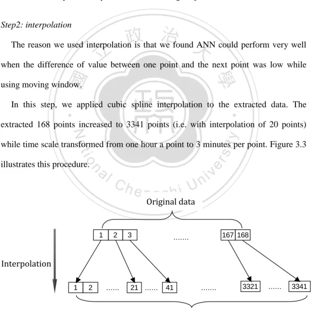
(30) 3.2. Experiment design In this study, the forecasting strategies are presented as the following steps: Step1: extract data Based on the benchmark study (Section 4.1), we extracted data series with an interval of one week (168 points from the electricity load hourly data), and 1005 points from daily gold price data as moving window length for training. In this section we took the hourly electricity load data as a testing subject. Step2: interpolation. 政治大. The reason we used interpolation is that we found ANN could perform very well. 立. when the difference of value between one point and the next point was low while. ‧ 國. 學. using moving window.. ‧. In this step, we applied cubic spline interpolation to the extracted data. The extracted 168 points increased to 3341 points (i.e. with interpolation of 20 points). y. Nat. n. al. er. io. illustrates this procedure.. sit. while time scale transformed from one hour a point to 3 minutes per point. Figure 3.3. Ch. engchi. i Un. v. Original data. 1. 2. 3. 167 168. ........ Interpolation 1. 2. ....... 21 ....... 41. ........ 3321. ....... 3341. Interpolated data Figure 3.3 The interpolation method. 29.

(31) Since the original data was based on hourly intervals, the interpolated points in step 2 are non-existent and unrealistic for forecasting purposes. If we wanted to forecast the value of the next hour accurately, we needed to forecast the fictitious points. We found that extrapolation could provide accurate forecasting results, but only to a certain extent. Therefore, our strategy was based on performing the extrapolation to an extent, and then forecasting residual virtual points. When a new virtual point was forecasted, we took this point and used it as real forecasted data to do the moving window forecasting procedure. After step 2, cubic spline extrapolation was applied to the new interpolated data.. very well and has good efficiency for program‘s working).. 學. ‧ 國. 治政 The number of extrapolation was decided empirically 大 (e.g. in this study we found that 立 interpolation with twenty points combine extrapolation with twelve points performs ‧. Step4: create a new data series for decomposition. Nat. sit. y. In step 4 we combined the interpolated data produced in step 2, with the. n. al. er. io. extrapolated points discarding the same amount as the extrapolated points in front of. i Un. v. the interpolated data (i.e. maintain the length of data with one week, see Fig.3.4).. Ch. Dropped data. 1. 2. ....... 13 ....... engchi. New data. 12. 21. ........ 3321. Interpolated data. ....... 3341. +. 1. 2. ....... 12. Extrapolated data. Figure 3.4 Create a new data series by interpolation and extrapolation. 30.

(32) Step5: EEMD and BPNN training The new data was created to decompose into IMFs through EEMD. After EEMD, the one week data was decomposed into meaningful IMFs which could be regarded as factors that influence the consumption of electricity. In this step, the IMFs which discarded last points were regarded as input data. The new data discarded the first point which was regarded as target data. For BPNN training, we put input and target data into a BPNN network, and the discarded the last IMFs‘ points which were used as input for the trained network to generate forecasting point (Fig.3.5).. 政治大 We combined the forecast 立point to the new data, discarded another point in front of. Step6: Moving window and forecasting. ‧ 國. 學. the new data, and update it again. After the newer data was updated, we repeated step 5 (i.e. the method is called moving window, see Fig.3.5) until the original hourly. ‧. point was forecasted. Once we got the forecasted hourly data, we then compared it. Nat. sit. y. with the real hourly data. In order to forecast the data of next hour, we took the real. n. al. er. io. data of next hour, added it into our data, and repeated step 3 to step 6.. Ch. engchi. i Un. v. 31.

(33) New data. . . .. 1. 2 2. Target data. 21 ....... ...... ....... 21 ...... 21 ....... ....... ........ 3321 3321. ...... ....... 3340 3340 3341. ‧ 國. 21 ....... al. 21 ...... 21 ....... Ch. 41. ........ 41 41. ....... ........ engchi Input. Input data (IMFs). 3342. ‧. ...... ....... predict. 學. 3 3. 41 41. . . .. n. Target data. ....... io. 2. 3340 . . .. 3341. Nat. Input data (IMFs). . . .. ....... 3341 . . .. 立. . . .. 3321. Input trained network 政治大. Input data (IMFs). 3. ........ . . .. Moving window. 2. 41. 3321. ....... 3341 . . .. ...... ....... 3341 3341 3342. y. . . .. ....... 3342 . . .. sit. 2. er. Input data (IMFs). 1. i Un. v. trained network. 3321 3321. predict 3343. 3342. Figure 3.5 Training Network by Moving Window Process. 32.

(34) 3.3. Statistical measures In this section we shall introduce various statistical measures that are used to analyze the IMF properties, and forecasting result performance. The measures used to analyze IMFs are mean periods, Pearson correlation coefficient, and power percentage. The measures used to see performance of forecasting results are RMSE, MAE and the standard deviation of error. These measures are presented as follows: Mean period The mean period which is used to see the cycle of an IMF is calculated by the. 政治大. inverse of mean frequency. The mean frequency is the average of ―instantaneous. 立. frequency‖. To calculate the instantaneous frequency, we apply HHT to the extracted. ‧ 國. 學. IMFs. In the following paragraph we will briefly introduce the HHT, proposed by. ‧. Huang et al. (1998).. For any arbitrary time-series data set X(t), we can always have its. y. Nat. n. al. er. io. sit. Hilbert-transform Y(t) as. Ch. engchi. i Un. v. Where p.v. indicates the Cauchy principal value. Then we use X(t) and Y(t) to form the complex conjugate pair, and get an analytic signal Z(t) as. Where. and. 33.

(35) Which a(t) indicates the amplitude varied with time, and (t) represents the phase also a function of time. The above is the best local fit of amplitude and phase-varying trigonometric function to the original time series data X(t). Now we can define the instantaneous frequency of Hilbert transform through the phase:. Therefore, the mean frequency F of an IMF can be presented as:. 立. 政治大. and the mean period T will be. ‧. ‧ 國. 學. Nat. sit. y. Notice: We didn‘t calculate the mean period of residue because it is a monotonic. n. al. er. io. function, so in this study we ignored the mean period of residue. Pearson correlation coefficient. Ch. engchi. i Un. v. The Pearson correlation coefficient, which‘s value always ranges from -1 to +1, is the most familiar measure used to detect the dependence between two quantities. The Pearson correlation +1 means a perfect positive linear relationship while -1 means a perfect negative linear relationship. As the value approaches zero, it means there is correlation and becoming almost uncorrelated. As it approaches -1 or +1, the correlation is stronger between two variables. Here the Pearson correlation coefficient ρ. XY. between two variables X and Y with expected values μ. deviations σ. X andσ Y. X and. μ. Y. and standard. is shown as follows: 34.

(36) Where E is the expected value operator and cov(X,Y) means covariance between X and Y. Power percentage Power percentage is a measure based on variance for detecting the weight of an IMF on the original data. A higher value of power percentage indicates a stronger. 政治大. weight an IMF is. The power percentage is defined as follows:. 立. ‧ 國. 學. Root mean square error and mean absolute error. ‧. Root mean square error (RMSE) and mean absolute error (MAE) are both useful. y. Nat. er. io. sit. quantities to measure how closely predicted or forecasted values are to the actual data, and are good measure of accuracy. The RMSE and MAE are given by:. n. al. Ch. engchi. i Un. v. Where R(t) indicates the real data at time t and P(t) means predicted data value at time t.. 35.

(37) Standard deviation of error The standard deviation of error in this study is the standard deviation calculated from the error between the predicted and real values of every hour. Using this measure, we can find the fluctuation of errors. A lower standard deviation indicates that the errors tend to be very close to the mean, whereas higher standard deviation indicates that the errors are spread out over a large range of values.. 立. 政治大. ‧. ‧ 國. 學. n. er. io. sit. y. Nat. al. Ch. engchi. i Un. v. 36.

(38) 4. Results and discussion 4.1. Benchmark study Before forecasting, we first did a benchmark study in order to choose the input data length. Table 4.1 shows some measures of the forecasting results of the 2011 gold price daily data which used four different data lengths as input. From this table we can see that the input data length with 1005 points and 754 points perform little better than 1255 points and 2759 points, and saved more time during training process. In addition, the data length with 1005 points was better than the 754 points because it may have contained more information. Therefore, we chose and fixed data length with. 治政 1005 points (i.e. time interval from 2007 to 2010) as our 大input data in this study. 立 ‧. ‧ 國. 學 er. io. sit. y. Nat. al. n. Table 4.1 Comparison between different input data length for forecasting of 2011 gold price 2000-2010. Ch. e n2006-2010 gchi. i Un. v. 2007-2010. 2008-2010. (2759points). (1255 points). (1005 points). (754 points). RMSE. 27.7. 34.2. 26.0. 26.1. MAE. 19.0. 21.1. 19.5. 19.0. Correlation coefficient. 0.978. 0.966. 0.981. 0.980. 20.2. 26.9. 17.2. 18.0. Standard deviation of error. 37.

(39) Similarly, for judging the suitable input length of electricity load data, we tested four different data lengths. The forecasting measure results of June 6, 2008, GCB10 are displayed in Table 4.2. The table shows that the data length with one-week performed the best depending on the measures. Although the length with two-weeks and three-weeks also had good performance, the time spent training doubled and tripled.. However, the measures of length which took only one-day perform so. poorly due to big error, occurring from 5:00 to 6:00. The case revealed that the time interval was too short for training, and from this short training, data may have caused the occurrence probability of big error, resulting possibly from a lack of information.. 治政 Based on the above reasons, the one-week data length 大 is the most suitable choice for a 立 training set which was used in this research. ‧. ‧ 國. 學. n. er. io. sit. y. Nat. al. Ch. engchi. i Un. v. 38.

(40) Table 4.2 Comparison between different input data length for forecasting of June 6, 2008 of GCB10 One day. One week. Two weeks. Three weeks. Hour. error. error%. error. error%. error. error%. error. error%. 0~1. 4.3. 0.81. 17.6. 3.88. 19.4. 4.28. 3.2. 0.71. 1~2. 2.8. 0.53. 13.8. 3.11. 16.7. 3.76. 2.5. 0.56. 2~3. 4.6. 0.87. 3.9. 0.89. 7.5. 1.71. 16.4. 3.74. 3~4. 2.6. 0.48. 5.4. 1.24. 15.7. 3.63. 8.1. 1.88. 4~5. 9.8. 1.86. 3.3. 0.76. 9.8. 2.24. 16.9. 3.86. 5~6. 334.1. 63.63. 13.4. 3.12. 17.1. 3.97. 8.2. 1.89. 6~7. 10.0. 1.86. 1.8. 0.40. 5.8. 12.6. 2.82. 7~8. 15.2. 2.48. 7.32. 31.9. 6.54. 8~9. 18.7. 2.52. 6.34 35.7 政治大 12.5 1.85 2.4. 1.29. 0.36. 19.9. 2.94. 9~10. 29.4. 24.6. 3.06. 41.2. 5.13. 32.3. 4.02. 10~11. 0.7. 0.08. 5.3. 0.62. 5.8. 0.68. 2.8. 0.33. 11~12. 52.4. 6.51. 6.3. 0.72. 7.9. 0.90. 8.3. 0.94. 12~13. 20.5. 2.49. 13.7. 1.59. 6.0. 0.69. 0.48. 13~14. 21.8. 2.61. 8.6. 1.00. 9.4. ‧. 4.2. 1.09. 3.3. 0.39. 14~15. 40.7. 5.01. 16.4. 1.83. 10.8. 1.21. 1.9. 0.21. 15~16. 7.6. 0.95. 16.4. 1.80. 17.0. 1.86. 13.6. 1.49. 16~17. 6.5. 0.82. 12.3. 1.40. 27.9. 3.17. 2.9. 0.33. 17~18. 39.0. 5.12. 0.52. 17.6. 2.13. 18~19. 5.5. 0.78. 0.48. 14.0. 1.87. 19~20. 3.9. 0.57. 2.27. 3.6. 0.52. 20~21. 8.3. 1.22. 3.6. 0.54. 0.1. 0.02. 10.9. 1.64. 21~22. 4.4. 0.69. 18.5. 2.86. 23.9. 3.69. 26.6. 4.10. 22~23. 1.2. 0.20. 13.3. 2.43. 15.2. 2.78. 30.8. 5.63. 23~24. 3.3. 0.58. 23.8. 4.89. 0.0. 0.00. 0.9. 0.19. y. sit. io. n. er. Nat. al. 學. ‧ 國. 立 3.73. 31.0. iv n C 21.0 2.80 3.6 hengchi U 3.3 0.48 15.9 7.6. 0.92. 4.3. RMSE. 70.8. 14.6. 16.9. 15.7. MAE. 27.0. 12.4. 13.3. 12.2. 66.9. 7.8. 10.6. 10.1. Standard deviation of error. 39.

(41) 4.2. The meaning of IMFs Electricity load data from NCCU The most important work in building an ANN forecasting model is the selection of input variables. In the past some researchers had collected different types of data as variables to input into ANNs for forecasting future data. For example, industrial production index, exchange rate, commodity price and interest rate are the variables used for financial stock market time series forecasting. Temperature, wind velocity, hourly and daily historical data are used for electricity load forecasting. However, as mentioned before, the EEMD method proposed by Huang et al. can decompose time-series data into several. 立. 治政 IMFs which have 大 its. own physical meaning.. Consequently, we can regard IMFs as factors which influence the data for. ‧ 國. 學. constructing an ANN model. The EEMD-Based neural network learning paradigm. ‧. has been used by Yu et al. (2008) to forecast world crude oil spot price data. For the. sit. y. Nat. above reasons, in this study we applied the EEMD-Based neural network learning. io. n. al. er. paradigm to forecast electricity load data.. i Un. v. Here we took an input data series for testing. The input data which length was one. Ch. engchi. week from May 30 to June 5, 2008 of General Building of NCCU was used to train the network for forecasting data of June 6, 2008, Friday. The decomposed IMFs and residue are shown in Figure 4.1. The measures of these IMFs are presented in Table 4.3. In the figure and table, we can see that the IMF7, IMF8 and the residue are the most important. The IMF7 period is close to one day (24 hour means the variability of one day). As we already know, the electricity load always has a regular pattern of high consumption during the day and low consumption at night. The phenomenon is also known as peak hour and off-peak hour. We can find that the consumption always noticeably increases at 8:00, and decreases after 22:00.We can also conjecture that 40.

(42) these fluctuations are determined by the activities and usage of the General Building. Original data. by faculty and students.. 1200 1000 800 600 400 200. C1. 20 0 -20. C2. 10 0 -10. 政治大. 0. 立. -10. 0 -100. 0. io. 1500 2000 every three minutes. al. n. 0 -100 500. C7. 1000. Nat. 100. C6. 500. 0. 2500. 3000. 3360. 3000. 3360. sit. C5. 100. y. -20. ‧. ‧ 國. 0. 學. C4. 20. er. C3. 10. Ch. engchi. i Un. v. -500. C8. 200 0 -200. C9. 20 0 -20. Residue. 800 700 600. 0. 500. 1000. 1500 2000 every three minutes. 2500. Figure 4.1 The IMFs for General Building of NCCU from May 30 to June 5, 2008. 41.

(43) Table 4.3 Measures of IMFs for General Building of NCCU from May 30 to June 5, 2008. Mean. Mean. Power. Pearson. period(Hour). period(Day). percentage(%). correlation. IMF1. 0.158. 0.007. 0.054. 0.017. IMF2. 0.289. 0.012. 0.020. 0.020. IMF3. 0.568. 0.024. 0.010. 0.014. IMF4. 1.414. 0.059. 0.052. 0.107. IMF5. 3.117. 0.130. 1.431. 0.152. IMF6. 6.431. 0.268. 1.824. 0.050. IMF7. 23.513. 0.980. 74.750. 0.857. IMF8. 86.408. 3.600. 17.913. 0.445. IMF9. 160.699. 立. Residue. 治 0.204 6.696 政大 2.829. 0.230 0.191. ‧ 國. 學. The IMF8, which is the second most important IMF, presents behavior of a. ‧. half-week pattern. The half-week pattern presents the highest consumption trend of. Nat. sit. y. the original data. The IMF9, which period is close to 7 days, presents the one-week. n. al. er. io. pattern and the property of difference between week-days and weekends. The residue,. i Un. v. also known as trend of data, presents the mean consumption trend of the week.. Ch. engchi. Compared IMF8 and residue, we can find that the highest consumption of Monday and Tuesday is higher than Wednesday and Thursday but the mean consumption of Wednesday and Thursday is more than Monday and Tuesday. The reason is that the arrangement of courses are centralized in certain sessions in Monday and Tuesday while the courses in Wednesday and Thursday are more but allocated to various sessions. Upon the IMFs‘ properties, the forecasting results are revealed in section 4.3.. 42.

(44) Gold price daily data Unlike the electricity load data, the daily gold price data didn‘t reveal any regularities. Gold price data is very similar to stock market series, meaning when the moving window shifts, the property of IMFs will change. But if we could take a long enough length of gold price data, we found that the trend was always the important one due to the obvious increase of gold price in past years. Moreover, a major reason for increase was inflation as well as the global financial crisis of the recent years. We took the daily price data from Jan, 2007 to Dec, 2010 as a testing subject.. The data. length (1005 points) was also the length of the moving window we used. The data was decomposed into seven IMFs. 立. 治政 as well as one residue 大. by EEMD (Figure4.2).. Furthermore, from Table 4.4, we can see that the most dominant component was the. ‧ 國. 學. residue, and the second most dominant, the IMF7. The Pearson correlation coefficient. ‧. of residue was 0.942 with the power percentage reaching up to 98%. Through this. sit. y. Nat. case, we validated that the trend was the most important influencing factor for gold. io. al. n. predicted. The performance is displayed in section 4.4.. Ch. engchi. er. prices. With the fixed window length of 1005 points, the daily gold price was. i Un. v. 43.

(45) data. C1. 20 0 -20. C2. 1500 1000 500. 20 0 -20. 2-Jan-08. 2-Jan-09 Day. 4-Jan-10. 30-Dec-10. ‧. ‧ 國. 立. 政治大. 學. Residue. C7. C6. C5. C4. C3. 50 0 -50 50 0 -50 50 0 -50 50 0 -50 200 0 -200 1500 1000 500 2-Jan-07. Nat. er. io. sit. y. Figure 4.2 The IMFs of historical gold price daily data from 2007 to 2010. al. n. iv n C Table 4.4 Measures of IMFs price daily data from 2007 to 2010 hfore gold ngchi U Mean period(Day). Power percentage(%). Pearson correlation. IMF1. 3.090. 0.119. 0.049. IMF2. 6.592. 0.080. 0.032. IMF3. 14.199. 0.137. 0.063. IMF4. 26.959. 0.233. 0.119. IMF5. 55.593. 0.444. 0.174. IMF6. 121.516. 0.857. 0.158. IMF7. 404.139. 7.630. 0.111. 98.105. 0.942. Residue. 44.

(46) 4.3. Forecasting performance This section shows our forecasting results. Below is a sample of forecasting performance for June 6, 2008 of GCB10 is shown in Table 4.5:. Table 4.5 Forecasted hourly load compared with actual load for June 6, 2008 of GCB10 Hour. Actual load (KWH). Forecasted load(KWH). Error. Error%. 0~1. 453. 470.6. 17.6. 3.88. 1~2. 444. 457.8. 13.8. 3.11. 2~3. 439. 442.9. 3.9. 0.89. 3~4. 432. 426.6. 5.4. 1.24. 4~5. 437. 3.3. 0.76. 5~6. 431. 13.4. 3.12. 1.8. 0.40. 31.0. 6.34. 12.5. 1.85. 24.6. 3.06. 9~10 10~11. 676. 688.5. 803. 827.6. 861. 866.3. 5.3. 0.62. 876. 6.3. 0.72. 13.7. 1.59. 8.6. 1.00. 16.4. 1.83. 16.4. 1.80. 12.3. 1.40. 12~13. 862. 848.3. 13~14. 859. 850.4. 14~15. 894. 15~16. 911. 16~17. 879. 17~18. 825. 832.6. 7.6. 0.92. 18~19. 751. 772.0. 21.0. 2.80. 19~20. 699. 695.7. 3.3. 0.48. 20~21. 667. 663.4. 3.6. 0.54. 21~22. 648. 666.5. 18.5. 2.86. 22~23. 546. 559.3. 13.3. 2.43. 23~24. 487. 463.2. 23.8. 4.89. 877.6. Ch. 927.4 e n g c891.3 hi U. sit er. n. al. y. 882.3. io. 457.0. Nat. 11~12. 488. ‧. 8~9. 444.2. 學. 7~8. 立 446. ‧ 國. 6~7. 433.7 政治大 417.6. v ni. RMSE. 14.6. MAE. 12.4. Standard deviation of error. 7.8. 45.

(47) In the above table, the error is the difference between forecasted value and actual value The error(%) is defined as below:. As we can see, the biggest error is 31 KWH. The error(%) is about 6.3% from 7:00 to 8:00, whereas the smallest error is only 2 KWH, and the error(%) is about 0.4% from 6:00 to 7:00. The RMSE, MAE and standard deviation of error are also presented in Table 4.5. The results illustrated in Figure 4.3 and Figure 4.4, and Figure. 政治大. 4.5 show the correlation between forecasted hourly data and actual hourly data.. 立. ‧ 國. 學. NCCU electric load forecasting of GCB10(General Building) 2008 6/6 Friday. ‧. 1000. n. al. er. io. sit. y. Nat. 900. KWH. 800. predicted hour predicted data real data. Ch. engchi. i Un. v. 700. 600. 500. 400. 0. 50. 100. 150. 200 250 300 Time(every 3 minutes). 350. 400. 450. 500. Figure 4.3 Forecasting performance for June 6, 2008 of GCB10 46.

(48) NCCU electric load forecasting of GCB10(General Building) 2008 6/6 Friday 1000 predicted hourly data real hourly data 900. KWH. 800. 700. 600. 政治大. 500. 立 0. 50. 100. 150. 200 250 300 Time(every 3 minutes ). 350. 400. 450. 500. 學. ‧ 國. 400. ‧. Figure 4.4 Forecasting performance of every hour for June 6, 2008 of GCB10. sit. n. al. 800. 700. Forecasted data(KWH). er. io. 900. y. Nat. Correlation between forecasted hourly data and real hourly data. 1000. Ch. engchi. i Un. v. 600. 500. 400. 300. 200. 100. 0. 0. 100. 200. 300. 400 500 600 Real data(KWH). 700. 800. 900. 1000. Figure 4.5 The performance of correlation between forecasted and actual hourly data 47.

(49) 4.4. Performance of ensemble average 4.4.1. Electricity load data from NCCU Since the BPNN aims to find the minimum mean square error function, the forecasting results try to approach the optimal result (i.e. global minimum). However, the program doesn‘t find minimum mean square error function every time; the results always deviate from the best or find the local minimum. Figure 4.6 shows the sketch of the error function surface. We can see that if the program finds a local minimum on the right of the global minimum, the error may be positive. In contrast, the local minimum on the left side may be a negative error. Therefore, we can apply the. 治政 ensemble average method on to the prediction result 大 to cancel out the error. We can 立 see that the performance by using ensemble average was better in this section. ‧ 國. 學. Error function. ‧. n. al. er. io. sit. y. Nat. Local minimum. Ch. engchi. i Un. v. Global minimum. Configuration. Figure 4.6 A diagrammatic sketch of the BPNN error function surface. Here we used the load data of May 22, 2008 of GCB10 for an analysis testing. We chose this data because its variation was not so regular compared with June 6, 2008 of GCB10, which had been analyzed in the proceeding text. In the Figure 4.7, we can see that the electricity load suddenly jumps over 1000KWH at the point 300 and 320 (i.e. 48.

(50) 14:00~16:00). It decreased gradually until about 820KWH at the point 380 (i.e. 18:00~19:00). Nevertheless, it suddenly jumped to 900KWH again the next hour. Although we could find the precise future trend, we couldn‘t get an accurate value in the suddenly changing points. On the other hand, the smooth, stable changed points could be predicted accurately. Based on these results, we took the data to see whether or not the forecasting performance would be better after the ensemble average. The forecasting results of the different ensemble levels are illustrated in Figure 4.7, Figure 4.8 and Figure 4.9. Figure 4.7 present forecasting results without the ensemble average. We can see that in the abruptly changed points such as 320 and 400, the large. 治政 error occurs, however, in Figures 4.8 and 4.9, which大 apply three and five times the 立 ensemble average respectively, we can clearly see that the forecasting results become ‧ 國. 學. better. In addition, Table 4.6 shows the comparison of quantity between these three. ‧. different ensemble average levels. The results without ensemble average have four. sit. y. Nat. points at which error percentage was over 5%. The RMSE, MAE and standard. io. al. er. deviation of error are 34.8, 21.0 and 28.4 respectively. When we apply the three times ensemble average to improve the results, the points which error percentages over 5%. n. iv n C were three, and the RMSE, MAE h and standard deviation e n g c h i U of error become 22.8, 17.2 and 15.4 respectively, all of which are better than the results without ensemble average. Even more, from the results using five times ensemble average, the points which error percentage was over 5% were only one. The RMSE, MAE and standard deviation of error were 18.5, 13.8 and 12.5 respectively, obviously better than the other two. In the comparison, we concluded that the forecasting error could be improved by applying the ensemble average method. However, a crucial drawback of this method is the large amount of time spent completing the process. For this reason, we aim to 49.

(51) reduce the program processing time in the future. The outlook will be discussed in the conclusion.. Load forecasting of GCB10(General Building) 2008 5/22 Thursday. 政治大. 1200. 立. 1100. KWH. 900. ‧. ‧ 國. 學. 1000. sit. n. al. er. io. 700. y. Nat. 800. 600. 500. 0. 50. predicted hour predicted data real data. 100. Ch 150. engchi. i Un. 200 250 300 Time(every 3 minutes). v. 350. 400. 450. 500. Figure 4.7 Forecasting performance for May 22, 2008 of GCB10,. without ensemble average. 50.

(52) Load forecasting of GCB10(General Building) 2008 5/22 Thursday ensemble(3) 1200 predicted hour predicted data real data. 1100. 1000. KWH. 900. 800. 700. 600. 0. 立. 50. 100. 150. 政治大 200 250 300 Time(every 3 minutes). 350. 400. 450. 500. 學. ‧ 國. 500. Figure 4.8 Forecasting performance for May 22, 2008 of GCB10,. with three times ensemble average. ‧. Load forecasting of GCB10(General Building) 2008 5/22 Thursday ensemble(5). sit. al. n. 1000. predicted hour predicted data real data. er. io. 1100. y. Nat. 1200. Ch. engchi. v. KWH. 900. i Un. 800. 700. 600. 500. 0. 50. 100. 150. 200 250 300 Time(every 3 minutes). 350. 400. 450. 500. Figure 4.9 Forecasting performance for May 22, 2008 of GCB10,. with five times ensemble average 51.

(53) Table 4.6 The performance comparison between different ensemble average levels no ensemble. ensemble(3). ensemble(5). error. error%. error. error%. error. error%. 0~1. 3.2. 0.60. 7.6. 1.43. 4.8. 0.89. 1~2. 0.6. 0.12. 4.1. 0.78. 3.4. 0.64. 2~3. 2.7. 0.52. 5.7. 1.08. 5.0. 0.96. 3~4. 0.6. 0.11. 0.5. 0.09. 1.8. 0.34. 4~5. 5.4. 1.04. 1.9. 0.36. 7.7. 1.48. 5~6. 4.4. 0.84. 5.6. 1.07. 1.6. 0.31. 6~7. 7.4. 1.38. 2.3. 0.42. 1.8. 0.33. 7~8. 41.6. 7.20. 38.0. 6.57. 30.9. 5.35. 8~9. 11.4. 1.51. 10.2. 1.34. 4.5. 0.60. 9~10. 12.7. 1.45. 10~11. 22.2. 1.59. 1.95. 4.1. 0.43. 13.8. 1.45. 15.8. 1.62. 21.9. 2.25. 18.5. 1.86. 45.2. 4.55. 3.7. 0.34. 17.8. 1.65. 119.8. 10.82. 0.1. 0.01. 14.9. 0.4. 0.04. 3.68. 11.6. 1.30. 18~19. 9.9. io. 1.20. 38.4. 4.68. 19~20. 81.3. 20~21. 52.2. 21~22. 19.0. 22~23. 2.6. 0.42. 29.0. 23~24. 1.4. 0.24. 17.7. n. al. 51.3. 18.7. 1.88. 34.0. 3.15. 12.7. 1.15. 9.2. 0.93. 17.0. 1.89. 39.1. 4.75. 45.1. 4.96. 1.2. 0.16. 4.6. 0.70. 4.74. 19.9. 3.26. 3.02. 22.9. 3.89. iv n C6.96h 18.2 2.42 U i e h n c g 2.89 34.4 5.25 8.96. 1.11. y. 33.0. 10.7. sit. 1.50. 17~18. Nat. 16~17. er. 15~16. 14.9. ‧ 國. 14~15. 0.65. 學. 13~14. 5.7. 立 18.6. 11~12 12~13. 政 24.5治 2.80 大 2.37 21.1 2.26. ‧. Hour. 5.65. RMSE. 34.8. 22.8. 18.5. MAE. 21.0. 17.2. 13.8. 28.4. 15.4. 12.6. Standard deviation of error. 52.

(54) 4.4.2. Gold price daily data In this section the forecasting results of gold price daily data without the ensemble average and five times ensemble average are both discussed. The two cases are illustrated in Figure 4.9 and Figure 4.10, with four mark influential events on the graph. For comparing, the RMSE of result without the ensemble average is 25.95, the MAE is 19.46, the standard deviation of error is 17.2 and the correlation coefficient between predicted data and actual data is 0.9813. The RMSE of result with five times ensemble average is 19.18 and the MAE is 14.28, both better than the performance of cases without ensemble average. The standard deviation of error is 12.84, meaning. 治政 that the error is more stable, and no large errors had occurred. 大 Finally, the correlation 立 coefficient was 0.9902, presenting a stronger correlation than the one without the ‧ 國. 學. ensemble average. The correlation between predicted price and real price of these two. ‧. cases are presented in Figure 4.11 and 4.13.. sit. y. Nat. The gold price has abruptly sky-rocketed in this past year, the main reason being. io. al. er. the European debt crisis. The euro against the U.S. dollar came to the lowest level on 30 Jan 2011 meanwhile the price of gold also came to a local minimum. This data. n. iv n C shows a strong correlation between gold price. However, in April 23, h currency e n g cand hi U. 2011, Greece applied for assistance to EU and IMF, and the gold price suddenly increased. It could be interpreted as people were looking for a hedge by buying large amounts of gold. Similarly, due to S&P reducing Greece‘s credit rating to CC on July 4 and the U.S.‘s later on August 5, as well as the world‘s stock market crashing as a result of worries about the U.S. second recession, the gold price experienced a dramatic rise. Our results present fine performance for prediction. However, after several times ensemble average, the results became even better. Upon these accurate results, maybe we can design a trading strategy in the future to see whether we can make a profit. 53.

(55) 1900. 1800. 4.23. Greece applied for assistance to the EU and the IMF. USD per ounce. 1700. 1600. 1.30. The euro against the U.S. dollar came to the lowest level in six months. 1500. 8.5. The second U.S. recession worries and world‘s stock market crash. 7.4. S&P cuts Greece‘s credit rating to CC, with a negative outlook. 政治大. 1400. 立. 1-Feb-11. 1-Mar-11. 1-Apr-11 3-May-11 1-Jun-11 Time(day). 1-Jul-11. 1-Aug-11. 1-Sep-11. 學. ‧ 國. 1300 4-Jan-11. predicted price actual price. Figure 4.10 Forecasting performance for 2011 gold price daily data,. ‧. without ensemble average. Correlation between forecasted daily data and real daily data. Forecasted data(USD per ounce). y. sit. n. al. er. io. 1800. Nat. 1900. 1700. Ch. engchi. i Un. v. 1600. 1500. 1400. 1300 1300. 1400. 1500. 1600 1700 Real data(USD per ounce). 1800. 1900. Figure 4.11 The performance of correlation between forecasted and actual daily data for. gold price daily data without ensemble average 54.

(56) 1900. 1800. USD per ounce. 1700. 4.23. Greece applied for assistance to the EU and the IMF 1600. 1500. 8.5. The second U.S. recession worries and world‘s stock market crash. 1.30. The euro against the U.S. dollar came to the lowest level in six months. 政治大. 1400. 立. 1-Feb-11. 1-Mar-11. 1-Apr-11 3-May-11 1-Jun-11 Time(day). predicted price actual price. 1-Jul-11. 1-Aug-11. 1-Sep-11. 學. ‧ 國. 1300 4-Jan-11. 7.4. S&P cuts Greece‘s credit rating to CC, with a negative outlook. Figure 4.12 Forecasting performance for 2011 gold price daily data,. ‧. with five times ensemble average. y. Nat. n. 1800. Forecasted data(USD per ounce). al. er. io. sit. Correlation between forecasted daily data and real daily data. 1900. Ch. 1700. engchi. i Un. v. 1600. 1500. 1400. 1300 1300. 1400. 1500. 1600 1700 Real data(USD per ounce). 1800. 1900. Figure 4.13 The performance of correlation between forecasted and actual daily data for. gold price daily data with five times ensemble average 55.