地理研究 第69期 民國107年11月
Journal of Geographical Research No.69, November 2018 DOI: 10.6234/JGR.201811_(69).0001
臺灣極端氣溫之季節潛在可預報度評估和氣候暖化的影響
Evaluation of Seasonal Potential Predictability of Temperature
Extremes in Taiwan and the Influence of Climatic Warming
翁叔平
aShu-Ping Weng
摘要
對季節氣候預測而言,每天的天氣變化是一種干擾,必須儘可能濾掉其影響。本研究提議用 一 種 數 值 方 法 可 鬆 弛 掉 對 季 節 內 天 氣 噪動 常 用 的 假 設 , 進 而 或 可 提 高 季 節 的 潛 在 可 預報 度 (Seasonal Potential Predictability; SPP)。提議的方法首先被應用於台灣百年長度,去掉線性趨勢的 測站月平均地表最高溫(Tmax)和最低溫(Tmin)。不必然需要假設為線性或定常才能模擬的天氣 噪動的月平均變異量,以及其在月與月之間的相關係數,一旦放掉通用的定常假設或註記為非零 值(假若相隔在一個月或以上的話,比如介於 1 月和 3 月),則數值解和直接使用日資料所得到的
估計值之間的一致性,與簡化方程下的解析解相比,將會好得很多。Tmax的SPP 估計值,除了冬
季略低之外,其他季節都較高。Tmin的SPP 估計值則是在秋冬兩季略低﹔但春夏較高。Tmax和Tmin
的總體平均的SPP 估計值(47.6%)約與解析解相當(46.2%),但兩者在個別測站和不同季節呈現 有明顯差異。 新方法被用到線性趨勢保留的原氣溫序列以便檢查氣候暖化對SPP 的影響。結果顯示暖化的 上升趨勢和增加的SPP 間的一致性,Tmin明顯高於Tmax。平均而言,夏季(冬季)Tmin的SPP 可 達86.3%(66.8%),比原先去掉線性趨勢得到的 SPP 高出 22.7%(20.3%)。其四季總體平均的 SPP 估計達 75.0%,與去掉線性趨勢後相比,增加了 27.4%。相反地,保留線性趨勢的 Tmax其SPP 的總體平均值(48.5%)則與先去掉線性趨勢後估計的 SPP 值,約略相等。不分季節的迴歸結果顯示, 暖化效率,定義為改變的SPP(保留線性趨勢減去去掉線性趨勢)與季節平均測站極端氣溫序列 的線性斜率,Tmin(Tmax)每百年增加1.0℃時,SPP 大約增加 16%(2%)。確實地,氣候暖化對 於極端氣溫的SPP,尤其是 Tmin,是外在的來源。 關鍵詞:潛在可預報度、氣候暖化、極端氣溫、臺灣 a 國立臺灣師範大學地理學系副教授(email: [email protected])
Abstract
The daily weather variability is considered as a noise for the seasonal climate prediction and thus its influence needs to be alleviated as much as possible. This study proposes a numerical method that relaxes the assumptions normally made in weather noise estimations within a season, thereby likely increasing seasonal potential predictability (SPP). The proposed numerical method is first applied to the centennial de-trended monthly-mean surface temperature maximum (Tmax) and minimum (Tmin) data in Taiwan’s measurement stations. The numerical solutions show that both the monthly mean variances of weather noise, not necessarily modeled by linear/stationary assumptions, and their inter-monthly correlations loosen the stationary assumption or register as non-zero values (if one month apart or even more, e.g. between January and March). Compared to the analytic solution of simplified equations, the numerical solutions in this studyg enerally have much better coherencies with those estimated directly using the daily data. The estimated SPP of Tmaxis slightly lower in winter but higher in other seasons. The estimated SPP of Tminis slightly lower in fall and winter but higher in spring and summer. The overall means in both Tmax and Tmin(47.6%) are comparable to the estimations of the analytic solution (46.2%), but significant differences appear at individual stations and seasons.
The warming trend effects on the SPP are examined by applying the new method to the trend series. The results showed that coherency between a warming trend and an increased SPP is significantly higher in Tmin than in Tmax. On average, the SPP of Tmin in summer (winter) is 86.3% (66.8%), and 22.7% (20.3%) higher than that of the de-trended SPP estimations. The overall mean of the trending SPP of Tminis around 75%, a 27.4% increase compared to the de-trended SPP. Conversely, the overall mean of the trending SPP of Tmax (48.5%) is similar to that of the de-trended estimate. The all-season regression shows that the warming efficiency, which is defined as the linear slope of the changed SPP (trend-remained minus de-trended) regressed on the trend values of seasonal-mean station temperature extremes, shown an increase of around 16% (2%) per 1.0 ℃ /100-yr warming for Tmin (Tmax). Conclusively, the climatic warming is an external source of SPP for temperature extremes, especially for the Tmin.
Keywords: Potential predictability, Climaticwarming, Temperature extremes, Taiwan
Introduction
Due to the high marine influence on air temperature, climate variability related to seasonal temperature extremes in Taiwan is generally not an attractive research subject in comparison with the precipitation variability. As the warming step progresses into the 21st century, this island nation has experienced prolonged heat waves in recent summers and sweeping cold surges in recent winters causing large temperature fluctuations and in turn increasing the risk for respiratory and cardiovascular mortality (Yang et al., 2009; Wu et al., 2011). Soaring heat waves under global warming (e.g. Meehl
and Tebaldi, 2004) and abrupt cold surges unanticipated by people who are already acclimatized to a warmer world (Mercer, 2003; Park et al., 2011) have dire socio-economic impacts (Brown, 2011). Such impacts can be managed through the provision of seasonal forecasts to some extent.
While using dynamical models and statistical methods to make seasonal forecasts, researchers desire to identify not only the sources of predictive skill but the sources of uncertainty as well. The slowly varying external forcings such as changes in solar insolation, sea surface temperature (SST), sea ice, soil moisture and greenhouse gases, may contribute to skillful predictions. Potential predictability can also arise from the slowly varying internal atmospheric dynamics (Frederiksen and Zheng, 2007) such as the stratospheric quasi-biennial oscillation, Arctic oscillation and other low-frequency climate modes with the associated variability being roughly stationary within a season. Here, the word “potential” is used to highlight the possibility that the persistence of internal atmospheric dynamics actually may not be predictable at the seasonal time scale due to imperfect models (Feng et al., 2014). The uncertainty arises mainly from the day-to-day weather variability, which is essentially unpredictable beyond two weeks (Lorenz, 1963). The extent to which the variance in the predictable component exceeds that of the unpredictable counterpart raises the seasonal potential predictability (SPP hereinafter) issue. Central to the SPP estimation is the assumption that the predictable and unpredictable components are independent of each other (Leith, 1973; Madden, 1976; see reviews by Palmer and Anderson, 1994; Zheng et al., 2000). While such an assumption is artificial, it allows useful progress to be made (Leith, 1973). With this idealized assumption, SPP can be defined as the fraction of the total interannual variability that is due to the predictable component (called slow component by Zheng and Frederiksen, 2004).
Two fundamentally different approaches are taken to estimate SPP. The first one uses a dynamic AGCM model with prescribed boundary conditions (mainly slowly varying SST) to generate a multi-member ensemble of climate realizations. All ensemble members are forced by the same boundary forcing but started from slightly different atmospheric initial states (e.g. Rowell et al., 1995; Shukla, 1998; Kumar and Hoerling, 2000; Shukla et al., 2000). The basic philosophy is that the spread of ensemble members can be used to quantify the weather noise variability, whereas the relative similarity among ensemble members is considered the atmospheric true response to the external forcing and thus can be used to quantify the potentially predictable component of variability. This dynamic approach has a particular advantage in detecting weak signals arising from SST forcing (Rowell, 1998), but has the disadvantage of relying primarily on the capability of a model that always has flaws.
The second approach involves estimating the weather noise component of seasonal variance from statistical models fitted to a single realization of atmospheric evolution and comparing it with the observed interannual variance in seasonal means to quantify SPP (e.g. Madden, 1976; Shukla and Gutzler, 1983; Zwiers, 1987; Zheng et al., 2000; Feng et al., 2014). This statistical approach has the advantage of relying on observation data alone and avoiding the problems due to the imperfect dynamic models. Such a purely observation based approach also indicates that it can contain other sources of
predictability, in addition to the SST forcing (Rowell, 1998). The primary disadvantage of this approach is that it requires the observed time series to be long enough to make the assumptions behind the employed statistical model valid. This will always be an issue.
Statistical methods usually require using daily time series to solidify the assumptions regarding the probabilistic behavior of the underlying stochastic process. Zheng et al. (2000, 2004) however proposed a variance analysis methodology based on using the monthly mean time series and moment estimations to quantify the weather noise variance within a specific season, and thereby SPP. From the data availability perspective, this is impressive given that the monthly record of meteorological variables is often much longer and more accessible than the daily information. Nevertheless, the proposed method heavily relies on stationarity assumptions in the monthly mean variances and inter-monthly correlations of weather noise to form a closed system of moment equations by which the analytical solution can be obtained. As noted by Zheng and Frderiksen (2004), while these assumptions are fairly true in the solstice seasons, their applicability in the equinox seasons needs to be justified.
More recently, Grainger et al. (2009) found that the monthly mean variances in weather noise within a specific season are not necessarily stationary, but to a first order vary linearly. They thus proposed a modification of the Zheng et al. (2004) method and used it to estimate Australian surface temperature extremes in all four seasons. To have the analytic solution, however, their modified method still assumes stationarity in the inter-monthly correlations of weather noise.
The purpose of this study is to further relax the linear assumption of monthly mean variances made in Grainger et al. (2009) and the stationary assumption of inter-monthly correlations made in Zheng et
al. (2000, 2004). A numerical approach is proposed to solve the complete moment equations of monthly
variances and inter-monthly correlations of weather noise, and thereby the SPP. This new method is applied to the centennial long surface temperature extremes record in Taiwan to test the validity of the aforementioned assumptions.
After describing the modified statistical model and numerical approach in detail and its connection with the earlier works in Sect. 2, Sect. 3 reports on its application to estimate the SPP in individual seasons for both de-trended and trend-remained surface maximum and minimum temperatures in Taiwan. Comparisons are made between the numerical solution based on the complete moment equations and analytical solution based on simplified equations. With the centennial long record available, this study (in Sect. 3.3) also examines the relationship between the SPP and warming trend, if it exists, and long term variability in SPP in the temperature extremes using a series of 60-yr sliding time window experiments. Discussion and summary are given in Sect. 4.
Data and Methodology
1.Data
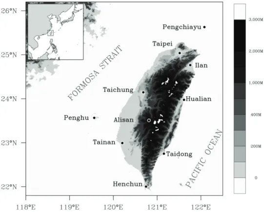
of daily surface temperature extremes recorded at operational synoptic stations since the early 20th century. Temperature records at seven stations with an overlapped 104-yr period, from December 1910 to November 2014, are employed in this study. Fig. 1 shows the geographical locations of these stations over the topography of Taiwan. As shown, they roughly constitute an observation network uniformly covering this subtropical island. Daily data are obtained from the atmospheric research databank in Taiwan (website: https://dbar.ttfri.narl.org.tw), which is maintained by the Taiwan Typhoon and Flood Research Institute (TTFRI) of National Applied Research Laboratories (NARL). Monthly-mean temperature extremes are calculated using these daily records. Interested readers can refer to Hung (2009) for the data quality problems and Weng (2010) for the recent trends in surface temperature extremes in Taiwan.
Fig. 1 Map of Taiwan with the geographical locations of the seven synoptic stations used in current study.
2. Statistical model
To make the subsequent comparisons easier, we used the same notation system as Zheng et al. (2000) to describe the statistical model employed in this study. That system was also used in the related works of Zheng and Frederiksen (2004), Grainger et al. (2009) and Ying et al. (2014), to name a few. We first removed the mean annual and semi-annual harmonics from the data (either daily or monthly)
using the spectral method proposed by Narapusetty et al. (2009). We then removed the long-term linear trend as well. The existence of a warming trend in a climate time series has been suggested as an additional source of potential predictability (e.g. Speer et al., 2006, Frederiksen and Zheng, 2007). We will scrutinize this notion in Sect. 3.3. Exploring the trend effects on the potential predictability will benefit from the long surface temperature maximum (Tmax hereinafter) and minimum (Tmin hereinafter) records in Taiwan. Treating it as a “regular” signal in the main body of the current study, removing the linear trend will facilitate weather noise component identification, which is essentially unpredictable at the interannual timescale.
As Zheng et al. (2000) noted, the statistical model for the observed monthly time series of an anomalous variable x at a particular season over a number of years is expressed in the following decomposition,
. (1)
Equation (1) decomposes the anomaly into a seasonal population mean in year y (y = 1, 2,…, Y, Y is the total number of years) and a residual monthly weather noise component from in month m (m = 1, 2, 3) within a given 3-month season. The standard seasons, December-to-February (DJF hereinafter), March-to-May (MAM hereinafter), June-to-August (JJA hereinafter) and September-to-November (SON hereinafter) are used in this study. Note that equation (1) implies that the month-to-month variability arises entirely from { 1, 2, 3}, which is assumed to be a stationary and
independent and identically distributed (i.i.d.) random vector with respect to year y.
We also denote the average taken over an independent variable (i.e. m or y) by replacing that independent variable with the subscript “o”. A seasonal mean can then be written as
, (2)
where the “total” field is the sum of the slow (i.e. predictable) component associated with the interannual variability of external forcing (and slowly varying internal dynamics) and the weather noise component which is unpredictable at the seasonal time scale. If the sample variance of , , can be known, then the SPP can be defined as (see Madden, 1976, Zheng and Frederiksen, 1999):
where the total interannual variability of the seasonal mean is estimated from the sample variance as
1
1 ∑ 1 2. (4)
In equation (4), 13∑3 1 , and 1∑ 1 .
As Grainger et al. (2009), let us denote the interannual variance of within a specific season as = 2, m = 1, 2, 3. The inter-monthly correlations, , , is then defined as
, , , , 1, 2, 3, , (5)
where , is the covariance between the weather noise components in month m and month n. Using the notation of equation (5), the interannual variance in seasonal mean weather noise component, , can be expressed as
1 3 1 3 2 1 9 1 2 3 2 1, 2 2, 3 1, 3 1 9 12 22 32 2 1 2 12 2 3 23 1 3 13 . (6)
Label E in equation (6) denotes the expectation value over all years.
3. Complete equations with numerical solution
To estimate , equation (6) indicates that we need to know the values of six parameters, i.e. { 1, 2, 3, 12, 23, 13}. However, based on equation (1), there also exist six sample moment equations linking the above six parameters as follows. The variance of 1 2, according to equations (1) and (5), can be estimated as
E xy1 xy2 2 E εy1 εy2 2 σ12 2σ1σ2φ12 σ 2 2 1 Y y 1 Y xy1 xy2 2 ∑ c1. (7a)
Similarly, the other five moment equations can be expressed as E xy1 xy2 xy1 xy3
E εy1 εy2 εy1 εy3
σ12 σ1σ2φ12 σ1σ3φ13 σ2σ3φ23 1
Y y 1
Y xy1 xy2 xy1 xy3
∑ c2, (7b)
E xy1 xy2 xy2 xy3 E εy1 εy2 εy2 εy3
σ1σ2φ12 σ22 σ1σ3φ13 σ2σ3φ23 1
Y y 1
Y xy1 xy2 xy2 xy3
∑ c3, (7c) E xy1 xy3 2 E εy1 εy3 2 σ12 2σ1σ3φ13 σ 3 2 1 Y y 1 Y xy1 xy3 2 ∑ c4, (7d)
E xy1 xy3 xy2 xy3 E εy1 εy3 εy2 εy3
σ1σ2φ12 σ32 σ2σ3φ23 σ1σ3φ13 1
Y y 1
Y xy1 xy3 xy2 xy3
∑ c5, (7e) E xy2 xy3 2 E εy2 εy3 2 σ22 2σ2σ3φ23 σ 3 2 1 Y y 1 Y xy2 xy3 2 ∑ c6. (7f)
Equations (7a)-to-(7f) describe a multivariable nonlinear system: 0, 1, 2,…, 6, with the unknown vector , 1, 2, 3, 12, 23, 13 and a constant vector 1, 2,…, 6 arising from the sample moments, which in principle can be solved numerically.
The conventional steepest descent method (Press et al., 1986) is employed in this study to solve the above numerical problem. We found that this method in most cases can achieve a satisfactory convergence speed as long as a proper initial guess can be provided (discussed next). We also found that it is more robust than the usual Newton-Raphson method (Press et al., 1986) in that the latter involves calculating the matrix inversion which may not always work well for ill-posed problems.
The steepest descent method seeks a vector that minimizes the function g:
g ∑ 1 2, (8)
where, in our case, n = 6, and . For the function g , the steepest descent direction in the n-dimensional hyperplane is given as g :
g 11 1 2 , ∑ 222 1 2 , , ∑ 1 2 ∑ 2 1 1 1 1 1 2 , (9)
where 1, 2,…,6 1, 2, 3, 12, 23, 13 , and symbolizes the Jacobian matrix of with the superscript T indicating the matrix transpose. Once the initial guess 0 is given, based on equation (9) we can determine the steepest descent direction g 0 and move an appropriate step size (> 0) in this direction to update 1 as:
1 0 g 0 . (10)
The above procedure will continue on until condition |g | τ or | 1 | τ is satisfied after m iterations. Here τ is a predefined tolerance error (τ = 1.0 x 10⁻¹⁰is used in this study).
There are various methods (see e.g. Sun and Yuan, 2006) that make an estimate of what a proper step size should be at a given iteration. A popular approach proposed by Barzilai and Borwein (1988) is used here to find the adaptive step size that minimizes function h():
where∆ 1 and∆ g g 1 . This is an approximation to the secant equation used in the quasi-Newton methods (cf. Section 10.7 in Press et al., 2007). Differentiating with respect toα, the above minimization in equation (11) leads to the following explicit formula for :
g g 1 1
g g 1 g g 1 . (12)
This approach works well because the necessary iterations are usually smaller than 10, provided that the initial guess is proper.
4. Simplified equations with analytical solution
In the works of Zheng et al. (2000, 2004), three assumptions were made to simplify the problem in hand: 1) the monthly variances within a specific season are stationary: 1 2 3 ; 2) the inter-monthly correlations are also stationary: 12 23 , and 3) the correlation of the weather noise components between the months is negligible if they are one month apart: 13 0. Under these assumptions, equation (6) becomes 92 3 4 , and can be arithmetically solved through the sets:
2 2 1 1[from equation (7a)] and 2 2 1
3 [from equation (7c)].
Grainger et al. (2009) argued that the monthly variances within a season are not necessarily stationary but tend to vary linearly to a first order. A linear model: 1 2 ; 3 2 , is thus introduced to accommodate the changes in observed variability. Note that 2 to ensure the positive standard deviations. After introducing the above linear modification, equations (7a), (7c) and (7f) constitute a closed system with three parameters: 2, in three equations and respectively become:
2 2 2 2 2 22 1, (13a)
2
2 2φ 1 3, (13b)
2 2 2 2 2 22 6. (13c)
After eliminating 2 andβ from equations (13a-13c), a cubic equation for is derived and the problem can be easily solved analytically (see Appendix in Grainger et al. 2009 for detailed formulae).
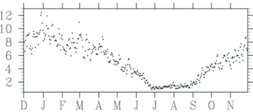
The linear variance assumption is reasonable but not universally realistic. Fig. 2 shows the daily sample variancesfor the 1910-2014 daily Tminat Taichung as a first-hand example (i.e. sample variances of {Ti, j, j = 1, 2, …, n}, i = 1, 2, …, 365, where sample size n = 104 years). A pronounced annual cycle
variances consist of the variability arising from both day-to-day weather noise and slowly varying components, a nonlinear behavior is evident in the December-to-June period, in addition to the sharp gradients during the transition seasons. It is also arguable regarding the stationary assumption of inter-monthly correlations and negligible contributions of 13. Nevertheless, the analytic solution obtained from the simplified equations indeed provides a good initial guess to solve the complete equations as will be demonstrated in Sect. 3.
Fig. 2 The scatter plot of daily sample variances (unit: ℃2) of the 1910-2014 daily Tmin at Taichung.
To compare the current results obtained from numerically solving the complete equations with those from analytically solving the simplified equations in the work of Grainger et al. (2009), it is instructive to estimate the monthly variances in the weather noise component directly from the daily records. Using daily data, Trenberth (1984) and Zheng (1996) estimated the monthly variances in the weather noise component (the “natural variability” in their terms) as
0 0 1 1 1 ∑ ∑ 1 2, (14)
where 0 is the time interval between independent observations:
0 1 2∑ 1 1 . (15)
Under the red noise assumption, the lag-t autocorrelation 1 , where 1 is the lag-1 day to day autocorrelation of daily sequence . The symbol is the number of days in the month m and is the seasonal mean of over the season that contains the month m. We used a Jackknife procedure to estimate 1 and its associated standard deviation (detailed in Buishand and Beersma, 1993).
It is also instructive to verify the stationary assumption of inter-monthly correlations using daily data. This is fulfilled using the formula in Zheng et al. (2000): , 1 900 11
the lag-1 autocorrelation of within both months: m and m+1. For a red noise time series, Zheng and Frederiksen (2004) has proved that , 1 is bounded between 0 and 0.1.
Results
1. Monthly variances and inter-monthly correlations
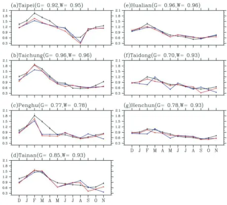
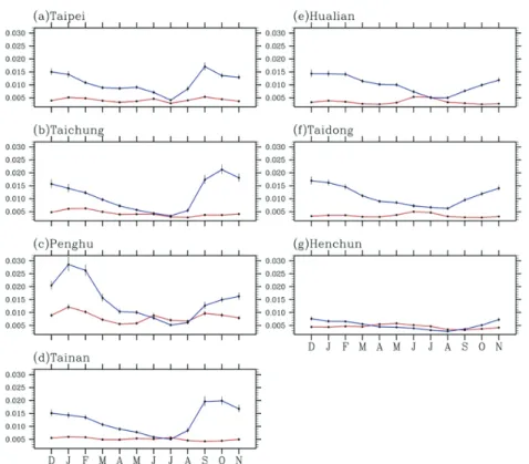
Fig. 3 shows the month-by-month standard deviations of the monthly variances in the weather noise component estimated from the daily records (black lines; along with the estimated one standard deviations), linear variance assumption (blue lines) and numerical solutions (red lines) for the centennial (December 1910 - November 2014) Tmaxrecords at seven stations. The results shown in the black lines clearly suggest that the stationary variance assumption, in general, does not hold at all stations and in all four standard seasons, though likely with an exception at Henchun during JJA (Fig. 3g) over which it is approximately true. Instead, a pronounced annual cycle of monthly variances with the maximum occurring in February and minimum occurring in August or September is evident, particularly at those stations located in the western plains of the Central Mountain Range (CMR; Figs. 3a-3d, c.f. Fig. 1). The accompanied annual amplitude is relatively large at Taipei and Taichung (Figs. 3a and 3b), which are located in the northwest portion of Taiwan, but becomes small at Taidong and Henchun (Figs. 3f and 3g) which lie towards the southeast/south direction. Note that the name Henchun in Chinese means that every day is a spring day.
On the other hand, monthly results based on the linear variance assumption, in some circumstances, are quite consistent with those based on the daily data. For example, its validity is high for the four western stations (Figs. 3a-3d) in DJF, for Taichung and Hualian (Figs. 3b and 3e) in MAM and for Taidong and Henchun (Figs. 3f and 3g) in JJA. Nevertheless, such an assumption has problems to detecting the nonlinearly increasing (decreasing) variance from January (July) to February (August) revealed in most (northwestern) stations. It even results in an incorrect slope sign at some stations during particular seasons (e.g. Fig. 3d for Tainan in JJA and SON seasons) as compared with the results based on the daily data (black lines).
Results from the proposed numerical method (red lines) are found to be able to alleviate the aforementioned problems to a large extent. In the aforementioned examples, numerical solutions attempt to relax the linear constraint and are capable of adjusting the erroneous slope sign. As a result, correlations (values shown inside the parentheses; note that the symbol G denotes Grainger’s linear assumption while W denotes Weng of current author’s numerical solution) between the monthly variances represented by the red lines and those represented by the black lines are generally higher compared with those between the blue lines and black lines. However, the “correction” effect seems to
be problematic at Penghu station (Fig. 3c). Both analytical and numerical methods result in lower correlations primarily due to the unfaithful estimates in MAM. Arguably, the proposed numerical method seemingly cannot converge well if the initial guess deviates too much from the prompt.
Fig. 3 The estimated month-by-month standard deviations of the weather noise component, , for the Tmax(unit: ℃)at seven synoptic stations. The black lines (along with the estimated 1.0 standard deviations) are the estimates using the daily data directly (i.e. equation (14)). The blue and red lines are the estimates using the monthly-mean data in terms of the linear variance assumption of Grainger et al. (2009) and using the numerical method of current study, respectively. See text for details. The symbols G and W denote Grainger and Weng, respectively.
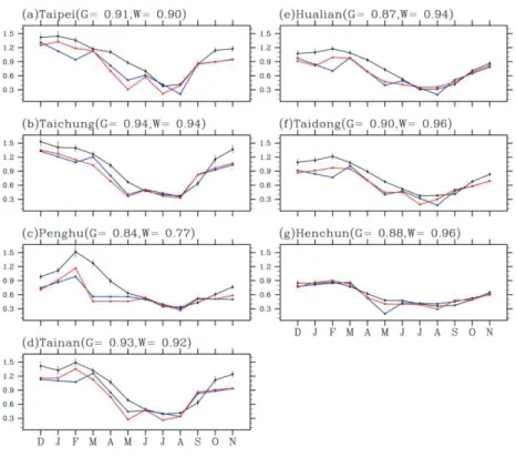
Similar behaviors are observed in the results of Tmin (Fig. 4). The stationary variance assumption is unrealistic for most stations, except at Henchun during DJF and JJA seasons. The linear variation assumption generally works well particularly in MAM, although it tends to overestimate the slopes. The “correction effect” of our numerical approach is most significant in DJF but likely functionless in SON. The results in Tmax, higher correlations in Tmin due to the proposed method are also found at eastern stations (Figs. 4e-4g). Again, the results from both analytical and numerical methods are problematic at Penghu station in MAM (Fig. 4c). Conclusively, the current numerical approach still heavily depends on the initial guess provided by the linear variances assumption.
Fig. 4 Same as Figure 3, except for Tmin(unit: ℃).
Using daily data the stationary assumption of inter-monthly correlations is examined in Fig. 5 for Tmax (red lines) and Tmin (blue lines) at seven stations. Although with some “bumps” in JJA and SON, the inter-monthly correlations for Tmax are fairly smooth at each station. However, this is not the case for Tmin. Rather, its validity is high for the eastern stations (Figs. 5e-5g) but is lower for the western stations (Figs. 5a-5d). We also found that, for Tmin, the inter-monthly correlations are relatively higher as well as variable during SON and DJF seasons but lower in MAM and JJA.We can, as Grainger et al. (2009) did, assess the induced error solely caused by this assumption in weather noise variance estimation (i.e. ) for Taiwan stations. The maximum difference between the adjacent inter-monthly correlations in a particular season is about 0.01 (after counting the uncertainty), which occurs at Penghu station in DJF for Tmin (between December and January, see Fig. 5c). If the true values satisfy 23
12 0.01 , then the estimated error in is 19 0.02 2 2 19 0.04 22 (under linear variance assumption, 3 2 , and 2). The error, based on the daily data estimates, is then around 1% of the trueV . In this regard, the stationary assumption for the inter-monthly correlation is relatively realistic for the Tmaxand Tminacross Taiwan’s stations.
Fig. 5 The daily data estimated month-by-month inter-monthly correlation of the weather noise component, ( , ), for Tmax (℃; red line) and Tmin (℃, blue line) at seven stations.
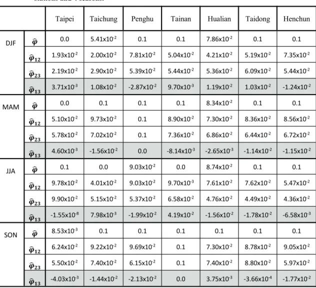
Using monthly data, the inter-monthly correlations of the weather noise component for Tmax estimated by both stationary assumption (i.e. in eq. 13) and the current numerical method ( 12, 23, 13) are tabulated in Table 1 for individual stations and seasons. As shown, although the differences between 12 and 23 are generally small in DJF and MAM, a larger 0.03 〜 0.04 difference, which is in the same order as 12/ 23, can be found at Penghu, Tainan and Taidong in JJA and/or SON seasons. Similar differences are also observed in the results for Tmin but occurred in DJF and MAM (not shown). Also note that, for the estimates in Tmax, a nearly 0.05 difference between and 12, which is comparable to 12 itself, can be found at Tainan and Taidong in DJF. As a result, the stationary assumption of inter-monthly correlations cannot be universally justified for this monsoonal island.
As for the 13, while many circumstances indeed have a value at least one order smaller than the accompanied 12/ 23 and thus it can be neglected, some cases in Table 1 (e.g. Tainan in JJA) actually have values that are in the same order as 12/ 23. In such cases, the contribution of the associated term (i.e. 1 3 13, see eq. 6) to cannot be ignored at all. The same conclusion is also obtained from the results for Tmin (not shown). In this respect, it is then suggested that we need to scrutinize this long-held notion: since day-to-day weather events are usually unpredictable beyond 10 days, two
weather noise components are irrelevant if their occurrences are one month apart (i.e. the third assumption mentioned in Sect. 2.4). We will discuss this later in Sect. 4.
Table 1 The monthly-data estimated inter-monthly correlations of Tmax obtained from the stationary inter-monthly assumption ( ) and numerical solutions ( , , ) for 7 stations and 4 seasons.
Taipei Taichung Penghu Tainan Hualian Taidong Henchun
DJF 0.0 5.41x10‐2 0.1 0.1 7.86x10‐2 0.1 0.1 1.93x10‐2 2.00x10‐2 7.81x10‐2 5.04x10‐2 4.21x10‐2 5.19x10‐2 7.35x10‐2 2.19x10‐2 2.90x10‐2 5.39x10‐2 5.44x10‐2 5.36x10‐2 6.09x10‐2 5.44x10‐2 3.71x10‐3 1.08x10‐2 ‐2.87x10‐2 9.70x10‐3 1.19x10‐2 1.03x10‐2 ‐1.24x10‐2 MAM 0.0 0.1 0.1 0.1 8.34x10‐2 0.1 0.1 5.10x10‐2 9.73x10‐2 0.1 8.90x10‐2 7.30x10‐2 8.36x10‐2 8.56x10‐2 5.78x10‐2 7.02x10‐2 0.1 7.36x10‐2 6.86x10‐2 6.44x10‐2 6.72x10‐2 4.60x10‐3 ‐1.56x10‐2 0.0 ‐8.14x10‐3 ‐2.65x10‐3 ‐1.14x10‐2 ‐1.15x10‐2 JJA 0.1 0.0 9.03x10‐2 0.0 8.74x10‐2 0.1 0.1 9.78x10‐2 4.01x10‐2 9.03x10‐2 9.70x10‐3 7.61x10‐2 7.62x10‐2 5.47x10‐2 9.90x10‐2 5.15x10‐2 5.37x10‐2 6.58x10‐2 4.76x10‐2 4.49x10‐2 4.36x10‐2 ‐1.55x10‐8 7.98x10‐3 ‐1.99x10‐2 4.19x10‐2 ‐1.56x10‐2 ‐1.78x10‐2 ‐6.58x10‐3 SON 8.53x10‐3 0.1 0.1 0.1 0.1 0.1 0.1 6.24x10‐2 9.22x10‐2 9.69x10‐2 0.1 7.30x10‐2 8.78x10‐2 9.05x10‐2 5.50x10‐2 7.40x10‐2 6.15x10‐2 0.1 7.40x10‐2 8.80x10‐2 5.97x10‐2 ‐4.03x10‐3 ‐1.44x10‐2 ‐2.13x10‐2 0.0 3.75x10‐3 ‐3.66x10‐4 ‐1.77x10‐2
2. Variance in weather noise and seasonal potential predictability (SPP)
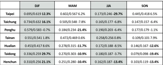
Variances in the weather noise component, , for Tmax estimated by a) the numerical method and b) linear variance assumption are shown in Table 2. Differences in between the two approaches are also shown as the percentages in changed ratios: (100 x )%. Both approaches show that, for all stations, the of Tmax is largest in DJF and generally smallest in SON, except at the Taipei station over which the smallest value appears in JJA. These two season-dependent extremes also display a geographical contrast. Larger (smaller) values of are found in those stations located in
the northwestern (southeastern) portion of Taiwan, consistent with the results found in the monthly variances (c.f. Fig. 3).
The changed ratios indicate that the current numerical method, compared to the analytical approach, tends to raise stations’ values in DJF but reduces them in other seasons. Taipei and Tainan are two exceptions, which show a moderate increased in SON. The increased wintertime variance ratio is about 14% on average for the northwestern stations (i.e. Taipei and Taichung), but can be up to 25% on average for the southeastern stations (i.e. Taidong and Henchun). The decreased variance ratio is generally around 10%, but is nearly 30% reduction at Taipei in JJA.
Table 2 The estimated variability of weather noise component(i.e. , unit: ℃2) for T
maxat stations using the proposed numerical method (values in the l.h.s. of slash) and the linear variance assumption (values in the r.h.s. of slash). The changed ratios are also expressed as percentages and in bold-faced when the absolute values exceed 10%.
DJF MAM JJA SON
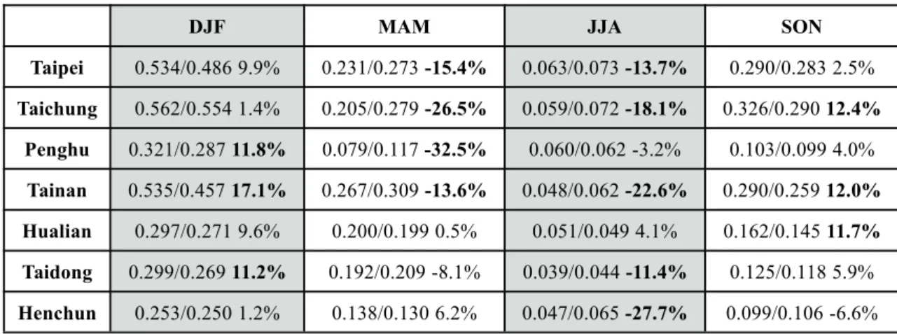
Taipei 0.695/0.619 12.3% 0.602/0.567 6.2% 0.173/0.246 ‐29.7% 0.445/0.418 6.5% Taichung 0.734/0.632 16.1% 0.505/0.548 ‐7.8% 0.165/0.177 ‐6.8% 0.147/0.157 ‐6.4% Penghu 0.579/0.583 ‐0.7% 0.184/0.234 ‐21.4% 0.190/0.203 ‐6.4% 0.177/0.179 ‐1.1% Tainan 0.551/0.541 1.8% 0.472/0.469 0.6% 0.258/0.256 0.8% 0.109/0.101 7.9% Hualian 0.453/0.417 8.6% 0.278/0.315 ‐11.7% 0.172/0.188 ‐8.5% 0.146/0.167 ‐12.6% Taidong 0.336/0.259 29.7% 0.270/0.303 ‐10.9% 0.180/0.187 ‐3.7% 0.079/0.098 ‐19.4% Henchun 0.310/0.256 21.1% 0.251/0.280 ‐10.4% 0.162/0.187 ‐13.4% 0.103/0.119 ‐13.4% Table 3 shows the respected results for Tmin. Both the numerical and analytical methods show that the estimated at each station is largest in DJF and smallest in JJA. As in the case of Tmax, the variance in weather noise in Tmin also shows a similar geographical bias: higher/lower values are found in the western/southeastern stations. As for the changed ratios, the proposed numerical method tends to increase the stations’ values in SON and DJF but decrease them in MAM and JJA. The reduced magnitude, ranging between -18% and -32%, is especially apparent at Taichung, Penghu and Tainan during the warm seasons, and for Henchun in JJA. Conclusively, after relaxing the constrained assumptions, the proposed numerical method in some circumstances does affect the previous weather noise variance estimates (thus SPP, see below), evident for the station Tmaxand Tminin Taiwan.
Table 3 Same as Table 2, except for Tmin.
DJF MAM JJA SON
Taipei 0.534/0.486 9.9% 0.231/0.273 -15.4% 0.063/0.073 -13.7% 0.290/0.283 2.5% Taichung 0.562/0.554 1.4% 0.205/0.279 -26.5% 0.059/0.072 -18.1% 0.326/0.290 12.4% Penghu 0.321/0.287 11.8% 0.079/0.117 -32.5% 0.060/0.062 -3.2% 0.103/0.099 4.0% Tainan 0.535/0.457 17.1% 0.267/0.309 -13.6% 0.048/0.062 -22.6% 0.290/0.259 12.0% Hualian 0.297/0.271 9.6% 0.200/0.199 0.5% 0.051/0.049 4.1% 0.162/0.145 11.7% Taidong 0.299/0.269 11.2% 0.192/0.209 -8.1% 0.039/0.044 -11.4% 0.125/0.118 5.9% Henchun 0.253/0.250 1.2% 0.138/0.130 6.2% 0.047/0.065 -27.7% 0.099/0.106 -6.6% The SPP results as a percentage of the total seasonal variability estimated using the numerical method and analytical solution in terms of the linear variance assumption (values inside the parentheses), are shown in the first rows of Tables 4 and 5 with respect to individual stations for the Tmax and Tmin, respectively. For the sake of providing a gross perspective, we also calculated the related annual-means, station-means and overall means.
In response to the changes in , relative changes in the SPP due to the employed numerical method indicate that, for the Tmax, it tends to lower the SPP in DJF, particularly for the northwestern (i.e. Taipei and Taichung) and southeastern (i.e. Taidong and Henchun) stations. The averaged reduction is nearly -10% therein compared to about -6% in the station-mean. In other seasons, our new approach tends to raise the SPP by about +4% in MAM, +6% in JJA and +2% in SON in the station means. Such overall promotions are especially evident at Hualian, Taidong and Henchun stations, which are more affected by the adjacent oceanic climate. Nevertheless, the situation at Taipei is different. While the SPP is reduced in MAM (-3.7%) and SON (-5.4%), it is significantly increased from 37.7% to 56.2% to reflect the large reduction in (c.f. Table 2).
Note that the station-averaged SPP estimated by the numerical approach is higher in the transitional MAM (51.6%) and SON (55.4%) seasons than in the DJF (43.9%) and JJA (39.3%) seasons. Also note that the Taipei and Taichung stations, which are located in the northwestern corner of Taiwan, have the lowest SPP estimates (33.5% and 36.9%) in the annual means. Over this region, weather is intermittently affected by the westerly disturbances almost throughout the year. The fast urbanization in both cities is another possible cause. The consequences of human activities such as heat island effect and polluted aerosols may interfere with nature processes leading to higher noise level during the daytime.The overall mean of estimated SPP in Tmaxis 47.6% over Taiwan.
Effects of the proposed numerical method on changing the SPP estimates of Tminare not negligible either. The proposed method tends to reduce the SPP in DJF (-4.4%) and SON (-3.7%), especially at the Tainan station (-9.1% in DJF and -8.5% in SON) in response to the largely increased (see Table
3). On the other hand, it tends to raise the SPP in MAM (+7.7%) and JJA (+6.1%), especially at the Taipei (+11.4%, in MAM), Taichung (+20.7%, in MAM), Tainan (+11.2, in JJA) and Henchun (+14.0%, in JJA) stations. The new method is apparently more efficient in raising the SPP during the warm seasons.
The station-wide SPP is higher in JJA (63.6%) but much lower in SON (35.0%). Among all stations, Taipei (70.3%) and Taidong (76.4%) stations in JJA, and Taipei (27.1%) and Tainan (19.4%) in SON, have the highest and lowest SPP estimates, respectively. As for the annual means, the highest (lowest) SPP of Tmin, 63.7% (37.3%), appears at the Penghu (Tainan) station. Note that the Penghu station is located in the middle of the Formosa Strait whereas the Tainan station is located in the wind shield as well as rain shadow region during the northeasterly monsoon seasons (c.f. Fig. 1), although the geographical distance between them is short. The overall SPP mean in Tmin is 47.6% over Taiwan, ironically matching the result in Tmax.
3. Trend effects on SPP and long-term SPP variations
To examine the long-term trend effects on the SPP estimation, we have conducted the same numerical analysis but kept the trend in the anomalous time series. The resultant SPP estimates of Tmax and Tmin are also tabulated in Tables 4 and 5 (in shaded rows), respectively. It is clear to see that, for Tmax, the trend-remained SPP are not always larger than the de-trended SPP, although the seasonal-mean Tmax at stations mostly have a warming trend (c.f. Fig. 6a). The coherent relationship between a warming trend and an increased SPP can be found in DJF at all stations and in JJA at some rural stations (e.g. Penghu and Henchun). It becomes controversial in MAM and SON across individual stations.
On the other hand, the coherency for Tmin significantly increases at all stations and in all seasons. In JJA the trend-remained SPP reaches 86.3% on average and 93.2% at Taidong. In DJF the estimated SPP is lower but still reaches 66.8% on average, which is 20.3% higher than the de-trended SPP. The overall mean of trend-remained SPP in Taiwan is around 75%, a 27% increase compared to the de-trended SPP.
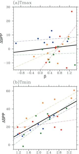
To further examine the warming trend “efficiency” in raising the estimated SPP of surface temperature extremes, the relationships between the seasonal trend slopes () for temperature anomalies and the corresponding differences in the SPP estimates (SPP), namely the trend-remained minus the de-trended estimated SPP across the employed seven stations, are shown as scatter plots in Fig. 6(a) for Tmax and Fig. 6(b) for Tmin. Different color codes represent different seasons: blue for DJF, green for MAM, red for JJA and golden brown for SON. The “efficiencies” represented by the linear regressions of SPP onto the values for individual seasons are also drawn as thin dashed lines using the same seasonal color codes. The thick solid black lines represent the “all-season” regressions.
Fig. 6 The scatter plots between the slopes of seasonal trends ( in abscissa, unit: ℃/100-yr) and the incremental SPP estimates (SPP in ordinate, unit: %) due to the inclusion of trend in the time series for the (a) Tmax(℃)and (b) Tmin(℃) at seven stations. The results in DJF, MAM, JJA, and SON seasons are marked by blue, green, red, and golden brown dots, respectively. Results of linear regression between the SPP and for individual seasons are also plotted as thin dashed lines using the corresponding seasonal color codes. The thick solid black line represents the all-season regression line.
In spite of the limited number of stations, Fig. 6 explores three salient features. First, a warming trend is more efficient in raising the SPP of Tmin than that of Tmax. The slopes of the all-season
regression indicate a 16.1% increase in SPP per 1.0℃ /100-yr warming in the former, but only a 2.0% increase per 1.0℃ /100-yr warming in the latter. Secondly, such a low efficiency in raising the SPP of Tmax, though generally true in other seasons, is betrayed by an upheaval during the JJA season (red dashed line in Fig. 6a). The efficiency becomes 21.4% per 1.0℃/100-yr warming in this season, which is contributed mainly by two rural stations, Penghu and Henchun (c.f. Table 4 and Fig. 1). Finally, the generally high warming trend efficiency in raising the SPP of Tminis overwhelmed by the degradation in JJA (red dashed line in Fig. 6b). The efficiency is less than 4.0% per 1.0 ℃ /100-yr warming therein, which is contributed mainly by two outliers, Taipei and Taidong (c.f. Table 5 and Fig. 1). Those two erratic results in JJA are intriguing and worth further discussion (see Sect. 4).
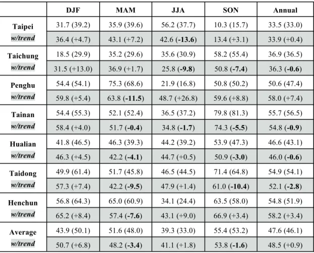
Table 4 The SPP estimations as a percentage of the total seasonal variability in terms of the numerical method (linear variance assumption) for Tmax at seven stations are shown in the first rows. Using the numerical method, results of the same analysis but keep the long-term trends in the time series are shown in the second rows (shaded areas) along with their differences (trend-remained minus de-trended estimates). Differences (in parentheses) between the trend-remained and de-trended estimated SPP are bold-faced if values in the former are smaller than those in the latter. The relative annual-mean, station-mean, and overall mean are also given.
DJF MAM JJA SON Annual
Taipei w/trend 31.7 (39.2) 35.9 (39.6) 56.2 (37.7) 10.3 (15.7) 33.5 (33.0) 36.4 (+4.7) 43.1 (+7.2) 42.6 (-13.6) 13.4 (+3.1) 33.9 (+0.4) Taichung w/trend 18.5 (29.9) 35.2 (29.6) 35.6 (30.9) 58.2 (55.4) 36.9 (36.5) 31.5 (+13.0) 36.9 (+1.7) 25.8 (-9.8) 50.8 (-7.4) 36.3 (-0.6) Penghu w/trend 54.4 (54.1) 75.3 (68.6) 21.9 (16.8) 50.8 (50.2) 50.6 (47.4) 59.8 (+5.4) 63.8 (-11.5) 48.7 (+26.8) 59.6 (+8.8) 58.0 (+7.4) Tainan w/trend 54.4 (55.3) 52.1 (52.4) 36.5 (37.2) 79.8 (81.3) 55.7 (56.5) 58.4 (+4.0) 51.7 (-0.4) 34.8 (-1.7) 74.3 (-5.5) 54.8 (-0.9) Hualian w/trend 41.8 (46.5) 46.3 (39.3) 44.2 (39.2) 53.9 (47.3) 46.6 (43.1) 46.3 (+4.5) 42.2 (-4.1) 44.7 (+0.5) 50.9 (-3.0) 46.0 (-0.6) Taidong w/trend 49.9 (61.4) 51.7 (45.8) 46.5 (44.5) 71.4 (64.8) 54.9 (54.1) 57.3 (+7.4) 42.2 (-9.5) 47.9 (+1.4) 61.0 (-10.4) 52.1 (-2.8) Henchun w/trend 56.8 (64.3) 65.0 (60.9) 34.1 (24.4) 63.5 (58.0) 54.8 (51.9) 65.2 (+8.4) 57.4 (-7.6) 43.1 (+9.0) 66.9 (+3.4) 58.2 (+3.4) Average w/trend 43.9 (50.1) 51.6 (48.0) 39.3 (33.0) 55.4 (53.2) 47.6 (46.1) 50.7 (+6.8) 48.2 (-3.4) 41.1 (+1.8) 53.8 (-1.6) 48.5 (+0.9)
Table 5 Same as Table 4, except for Tmin.
DJF MAM JJA SON Annual
Taipei w/trend 35.3 (41.1) 37.9 (26.5) 70.3 (65.4) 27.1 (28.7) 42.7 (40.4) 65.8 (+30.5) 66.5 (+28.6) 90.0 (+19.7) 79.1 (+52.0) 75.3 (+32.6) Taichung w/trend 46.2 (46.9) 41.8 (21.1) 57.7 (48.8) 36.7 (43.8) 45.6 (40.2) 64.2 (+18.0) 54.7 (+12.9) 83.6 (+25.9) 73.6 (+36.9) 69.0 (+23.4) Penghu w/trend 60.2 (64.5) 83.8 (75.8) 57.2 (55.9) 53.7 (55.5) 63.7 (62.9) 69.9 (+9.7) 82.2 (-1.6) 77.1 (+19.9) 73.4 (+19.7) 75.7 (+12.0) Tainan w/trend 37.4 (46.5) 31.9 (21.1) 60.6 (49.4) 19.4 (27.9) 37.3 (36.2) 70.0 (+32.6) 72.5 (+40.6) 92.3 (+31.7) 80.2 (+60.8) 78.8 (+41.5) Hualian w/trend 49.4 (53.9) 32.2 (32.5) 57.8 (58.8) 29.1 (36.8) 42.1 (45.5) 65.8 (+16.4) 64.5 (+32.3) 90.4 (+32.6) 75.9 (+46.8) 74.2 (+32.1) Taidong w/trend 47.0 (52.3) 38.2 (32.6) 76.4 (73.2) 34.7 (38.3) 49.1 (49.1) 70.0 (+23.0) 72.7 (+34.5) 93.2 (+16.8) 85.5 (+50.8) 80.3 (+31.2) Henchun w/trend 50.3 (50.8) 52.5 (55.2) 64.9 (50.9) 44.1 (39.8) 53.0 (49.2) 62.1 (+11.8) 63.9 (+11.4) 77.8 (+12.9) 73.7 (+29.6) 69.4 (+16.4) Average w/trend 46.5 (50.9) 45.5 (37.8) 63.6 (57.5) 35.0 (38.7) 47.6 (46.2) 66.8 (+20.3) 68.1 (+22.6) 86.3 (+22.7) 77.3 (+42.3) 74.7 (+27.1) The above features, on one hand, suggest the existence of an “embedded barrier” for the warming trend of Tmaxto promote the associated SPP. On the other hand, they concur with earlier studies that the warming trend is an external source of SPP (e.g. Frederiksen and Zheng 2007). This notion is especially true for Tmin, according to the current study. We may then wonder what would be the long-term SPP behavior if the “regular” warming trend is excluded in advance.
Using the proposed numerical method, the above question can be partly answered by estimating the SPP from serial 60-yr sliding time windows, beginning from the first window: 1911-to-1970 and each time shifting one year forward within the de-trended centennial-long records of temperature extremes until reaching the final window: 1955-to-2014. The choice of a 60-yr window (i.e. 60 samples) is decided by the stability consideration of the employed numerical algorithm. We found that the convergence of numerical solution is problematic as the number of iterations often exceeds 100 if the sample size is too small.
Figs. 7 and 8 show the resulting de-trended SPP time series for the Tmaxand Tminat seven stations and in four seasons, respectively. Note that few SPP time series still display disconnected segments due
to the aforementioned convergent problem. Despite fluctuations the de-trended SPP of Tmax in DJF generally remains stable at most stations (blue lines in Figs. 7a-7f), although Taipei has a long-term increasing tendency and Taichung and Tainan (Taidong) show(s) a recent decreasing (increasing) signal. The SPP series at Tainan has shown a decreasing trend in recent years (blue line in Fig. 7d). A similar decrease also appears at Penghu but it occurs in MAM (green line in Fig. 7c). In that season, four stations, Tainan, Hualien, Taidong and Henchun, express a slowly decaying tendency (green lines in Figs. 7d-7g). On the other hand, most stations express a slowly increasing tendency in JJA (red lines in Fig. 7b for Taichung, and 7e-7f for Hualian, Taidong and Henchun). Here, a contrasting decreasing tendency is found at Tainan (red line in Fig. 7d). The behaviors of the de-trended SPP at Taipei and Penghu stations are similar: an increasing tendency switches to a decreasing tendency in recent years (red lines in Figs. 7a and 7c). Interestingly, the switched tendency in JJA is accompanied by a nearly concurrent but increasing tendency in SON at these two stations (golden brown lines in Figs. 7a and 7c). Similar changes leading to an increase in de-trended SPP in recent years also appear at Taichung, Hualian and Taidong (golden brown lines in Figs. 7b, 7e and 7f).
Fig. 7 The long-term changes of de-trended SPP of seasonal mean Tmax ( ℃ , blue lines: DJF, green lines: MAM, red lines: JJA, golden brown lines: SON) at seven stations in terms of the 60-year sliding time windows.
As in the case of Tmax, the de-trended SPP time series of Tminare quite stable in DJF (blue lines in Figs. 8a-8g), although a recent increased signal is observed at Tainan, Hualian and Taidong. In contrast, the series in MAM show a nearly-concurrent decreasing tendency at most stations (green lines in Figs. 8a-8f), except at Henchun which is quite stable (green line in Fig. 8g). The decreasing tendency in MAM extends into JJA especially at Tainan and Taidong (red lines in Figs. 8d and 8f). While steady most of the time, the de-trended SPP at Taichung and Penghu (red lines in Figs. 8b and 8c) quickly decreased in recent years. In SON, however, these behaviors are controversial among stations. While a recent increasing signal appears at four western stations (Taipei, Taichung, Penghu and Tainan; golden brown lines in Figs. 8a-8d), a slowly decreasing signal superimposed on the low-frequency fluctuations can be found at Hualian and Taidong (golden brown lines in Figs. 8e-8f). Meanwhile, there is a steadily increasing signal at Henchun after 1990s (golden brown line in Fig. 8g). Interpretations on the above results will be given later.
Discussion and Summary
This study proposes a numerical method to estimate the variance in weather noise from monthly data within a specific season, and thereby the associated SPP. Applying it to the centennial long Tmaxand Tmin records in Taiwan, the results allow us to test the degree of fidelity of three assumptions made behind the usual analytical method in a monsoonal climate regime.
Firstly, the month-by-month variances in weather noise are not stationary and linear. The numerical method relaxes the linear assumption and results in a better coherence with the direct daily estimates. Secondly, the stationary assumption of inter-monthly correlations is less realistic in JJA and SON for Tmax and in DJF and MAM for Tmin, which are qualitatively consistent with the direct daily data estimates. Finally, the correlations between two months which are one month apart, i.e. the 13, are not negligible in some cases. This non-zero 13 implies the existence of some low-frequency weather noise signals regularly visiting the same place at least for a considerable number of years. Indeed, the idea of fast annual cycle has been proposed (LinHo and Wang, 2002) to represent the climatological intraseasonal oscillation (CISO, Wang and Xu, 1997) resident in the East Asian summer monsoon regions. During the boreal summer the seasonal march of the East Asian subtropical rainfall band (Meiyu in China and Baiu in Japan; e.g. Hsu et al., 2014) is best described by the CISO activity, which takes about two months to advance northward from the northern part of the South China Sea in the middle of May to northern China by the end of July (e.g. Liu et al., 2008). The presence of a significant negative 13 value in some cases, which contributes to a decreased variance of weather noise and thus an add-on source of SPP, could reflect the passage of the alternative dry and wet phases of CISO over Taiwan. On the other hand, a significant positive 13 value likely signifies the prolonged residence of CISO activity. Put together, in a monsoonal environment the zero 13 assumption should be judged with cautions instead of an ad hoc decision.
The estimated weather noise componentsof Tmax (Tmin) are large for stations in the northwestern (western) portion of Taiwan in DJF but relatively small for stations to the southeast in SON (JJA). Such a spatiotemporal contrast is attributable to the combined effects of prevailing wintertime westerly disturbances, the barrier role of CMR and thermal adjustments (e.g. through the sea breeze circulation) from the adjacent Pacific Ocean during the summertime.
The proposed numerical approachincreases the estimates of Tmax (Tmin) in DJF (DJF and SON) but reduces them otherwise (in MAM and JJA). The resultant SPP changes in wintertime Tmax then show a -6% reduction on average, which are in contrast with the widespread increases in other seasons (c.f. Table 4). Note the different response at Taipei in JJA. In response to the large decrease of , our new approach significantly increases the SPP of Tmax (from 37.7% to 56.2%), which is most welcome considering its implications for the potential socio-economic benefits. As for the Tmin, the new method generally reduces the SPP in cold DJF and SON seasons but raises it in warm MAM and JJA seasons. Such a tendency in reducing the SPP of Tmin in cold seasons is intentionally not what we
desire.
Annually, the numerical method shows relatively low seasonal-averaged SPP of Tmax at Taipei (33.5%) and Taichung (36.9%). Both cities are located in the northwestern portion of Taiwan. As well recognized, weather in this region is intermittently affected by the mid-latitude westerly disturbances almost throughout the year. The fast urbanization in both cities is another possible cause. As for the Tmin, the highest and the lowest SPP, 63.7% vs. 37.3%, appear at Penghu and Tainan, respectively. Although the geographical distance is short, Penghu is located in the middle of the Formosa Strait whereas Tainan is located in the wind shield as well as rain shadow (windward) region during the northeasterly (southwesterly) monsoon season. In Taiwan, the overall means of SPP in both Tmaxand Tminare 47.6%.
The results of trend effect examination showed that the coherency between a warming trend and an increased SPP is significantly higher in Tmin than in Tmax. The overall mean of trend-remained SPP for Tminin Taiwan is around 75%, a 27% increase compared to the de-trended SPP. On the other hand, the overall mean of trend-remained SPP for Tmax(48.5%) is roughly equal to that of the de-trended estimate (47.6%).Fig. 6 further examined the trend efficiency on the SPP, which is defined as the linear slope of changed SPP (SPP; trend-remained minus de-trended estimates) regressed on the linear trend values () of seasonal-mean temperature extremes of the employed stations. The estimated efficiency of all-season regression is 16.1% (2.0%) per 1.0℃/100-yr warming for Tmin(Tmax).
When the world is warming, the hydrological cycle is becoming more active. The role of the resultant cloud seems to play a different role from day to night in affecting the Tmax and Tmin, respectively. The increasing SPP of Tmin, which is in accordance with the increasing nighttime cloud amount (Weng, 2010), suggests the stabilized role (i.e. negative feedback) of hydrological cycle during the nighttime hours. While the surface cools down after sunset, the blanket effect of nighttime cloud tends to warm the lower troposphere thereby increasing the atmospheric stability and SPP. In SON, the above effect may reach its climax when the water vapor is profoundly supplied from the warm oceans. Note that in western north Pacific, the SST reaches its maximum in September. On the other hand, the almost unchanged SPP of Tmax, which is also in accordance with the controversial change of daytime cloud amount in different stations and different seasons (Weng, 2010), indicates that the response of daytime hydrological cycle is not unified yet but tends to be case dependent.
We have noticed that the trend efficiency in JJA drops to 4.0% (increases up to 21.4%) per 1.0℃ /100-yr warming for Tmin (Tmax), mainly attributable to the unusual behaviors at Taidong and Taipei (Penghu and Henchun). Note that in JJA Taidong and Taipei rank at the top two stations of de-trended SPP of Tmin (c.f. Table 5) whereas Penghu and Henchun have the lowest de-trended SPP of Tmaxamong stations. It seems that the high (low) de-trended SPP at former (later) two stations leaves no (plenty) room for the warming trend to increase the de-trended SPP further and our question becomes: why are the de-trended SPP of Tmin(Tmax) at Taidong and Taipei (Penghu and Henchun) so high (low). Taidong is located in the exit region of the East Rift Valley of Taiwan. On summer nights the local weather is controlled by the downslope winds from the CMR to the west and frequent foehn events induced by the
prevailing southwestlies. Taipei is located in a basin bounded by the Yangming Mountain to the north/northwest andthe Xueshan Mountain Range to the south/southeast. The downdraft associated with the prevailing easterlies stabilizes the nighttime air aloft. On the other hand, Penghu and Henchun are two islandic/rural cities deeply affected by the adjacent open oceans. Local weather on summer days is controlled by the sea breeze circulation. Both cities have relatively low mean seasonal-mean Tmax but high standard deviation in seasonal-mean Tmax. Put together, it suggests that the interaction between local topography and monsoon winds could be an influential factor in the SPP of temperature extremes.
Results of the 60-yr sliding time window analysis show the existence of long-term variability in de-trended SPP time series for both Tmaxand Tmin. The SPP series in both Tmaxand Tmin are more stable in DJF. Since the linear trend has been removed, such stability may be in response to the dominance of the warming trend over other factors in supporting the SPP during boreal winters. Notwithstanding, because it is only the linear part of trend removed, the eccentric de-trended SPP series such as the existence of long term tendency and recent increasing/decreasing tendency found at different stations and in different seasons may in parts signify the nonlinearity of warming/cooling trends in temperature extremes (Weng 2010). On the other hand, the de-trended SPP series at some stations in some seasons show a flip-flop between the increasing and decreasing tendency, or vice versa. This implies that factors other than the long term trend, such as the phase of atmospheric low-frequency modes (e.g. Arctic Oscillation; c.f. Lorenz, 1951, Thompson and Wallace, 1998; Pacific Decadal Oscillation; c.f. Yu et al., 2015), multi-decadal ENSO variability (e.g. Wang, 1995; Wu and Wang, 2002) and variability of CISO possibly interacting with the ENSO and atmospheric low-frequency modes (e.g. Ding, 2007), could contribute to the long term variability of SPP. For example, the CISO promotes the summertime SPP in Taiwan, and its variabilitywould disturb its promising signal. For practical prediction needs, it would be of interest to understand thesepossible sources of SPP and how the variations in them can affect the SPP of local climates. Using the proposed numerical method, the above tasks are underway and the results will be reported in future papers.
Acknowledgment
The author wishes to thank Mr. Chen-Dau Yang for the figures preparation. This study was sponsored by the Ministry of Science and Technology of Taiwan under Grants MOST106-2621-M-865-001-.
References
Barzilai, J., and Borwein, J. (1988). Two-point step size gradient methods, IMA Journal of Numerical
Analysis, 8: 141-148.
Brown, L. (2011). World on the edge: how to prevent environmental and economic collapse. W. W. Norton, New York.
Buishand, T.A., and Beersma, J.J. (1993). Jackknife tests for differences in autocorrelation between climate time series. Journal of Climate, 6: 2490-2495.
Ding, Y.H. (2007). The variability of the Asian summer monsoon. Journal of the Meteorology Society of
Japan, 85: 21-54.
Feng, X., Delsole, T., and Houser, P. (2014). Comparison of seasonal potential predictability of precipitation. Journal of Climate, 27: 4094-4110.
Frederiksen, C.S., and Zheng, X. (2007). Variability of seasonal-mean fields arising from intraseasonal variability. Part 3: Application to SH winter and summer circulations. Climate Dynamics, 28: 849-866.
Grainger, S., Frederiksen, C.S., and Zheng, X. (2009). Estimating the potential predictability of Australian surface maximum and minimum temperature. Climate Dynamics, 32: 443-455.
Hsu, H.H., Zhou, T., and Matsumoto, J. (2014). East Asian, Indochina and western north Pacific summer monsoon: An update. Asia-Pacific Journal of Atmospheric Sciences, 50: 45-68.
Hung, C.W. (2009). Temperature discontinuity caused by relocation of meteorological stations in Taiwan. Terrestrial, Atmospheric and Oceanic Sciences, 20: 607-617.
Kumar, A., and Hoerling, M.P. (2000). Analysis of a conceptual model of seasonal climate variability and implications for seasonal prediction, Bulletinof American Meteorological Society, 81: 255-264. Leith, C.E. (1973). The standard error of time-average estimates of climatic means. Journal of Applied
Meteorology, 12: 1066-1069.
LinHo, and Wang, B. (2002). The time-space structure of the Asian-Pacific summer monsoon: A fast annual cycle view, Journal of Climate, 15: 2001-2019.
Liu, J., Wang, B., and Yang, J. (2008). Forced and internal modes of variability of the East Asian summer monsoon. Climate of the past Discussions, 4: 225-233.
Lorenz, E.N. (1951). Seasonal and irregular variations of the Northern Hemisphere sea-level pressure profile. Journal of Meteorology, 8: 52-59.
Lorenz, E.N. (1963). Deterministic nonperiodic flow. Journal of Atmospheric Sciences, 20: 130-141. Madden, R.A. (1976). Estimates of natural variability of time averaged sea level pressure. Monthly
Weather Review, 104: 942-952.
Meehl, G.A., and Tebaldi, C. (2004). More intense, more frequent, and longer lasting heat waves in the 21stcentury. Science, 305: 994-997.
Narapusetty, B., Delsole, T., and Tippett, M.K. (2009). Optimal estimation of the climatological mean.
Journal of Climate, 22: 4845-4859.
Palmer, T.N., and Anderson, D.L.T. (1994). The prospects for seasonal forecasting: A review paper.
Quarterly Journal Royal Meteorological Society, 120: 755-793.
Park T.W., Ho, C.H., Yang, S., Jeong, S.J., Choi, Y.S., Park, S.K., and Song, C.K. (2011). Different characteristics of cold day and cold surge frequency over East Asia in global warming situation.
Journalof Geophysical Research, 116: 1-12.
Press, W.H., Fannerty, B.P., Teukolsky, S.A., and Vetterling, W.T. (1986). Numerical Recipes: The Art of
Scientific Computing. 1st ed. New York, Cambridge University Press, 848 pp.
Press, W. H., Teukolsky, S.A., Vetterling, W.T.,and Flannery, B.P. (2007).Numerical Recipes: The Art of Scientific Computing. 3rded. New York, Cambridge University Press, 1256pp.
Rowell D.P. (1998). Assessing potential seasonal predictability with an ensemble of multidecadal GCM simulations. Journal of Climate, 11: 109-120.
Rowell, D.P.,Folland, C.K., Maskell, K., and Waed, N. (1995). Variability of summer rainfall over tropical north Africa (1906-92). Observations and modeling. Quarterly Journal Royal
Meteorological Society, 121: 669-704.
Shukla, J.S. (1998). Predictability in the midst of chaos: A scientific basis for climate forecasting,
Science, 282: 728-731.
Shukla, J.S., and Coauthors (2000). Dynamical seasonal prediction. Bulletin of American
Meteorological Society, 81: 2593-2606.
Shukla, J.S., and Gutzler, D.S. (1983). Interannual variability and predictability of 500-mb geopotential heights over the Northern Hemisphere. Monthly Weather Review, 111: 1273-1279.
Speer, K., Cassou, C., and Minvielle, M. (2006). Influence of Indian Ocean warming on the southern hemisphere: atmosphere and ocean circulation. In: Proceedings of 89 ICSHMO, Foz do Iguacu, Brazil, April 24-28, INPE, pp 455-461.
Sun, W., and Yuan, Y.X. (2006). Optimization theory and methods: nonlinear programming. Springer-Verlag.
Thompson, D.W.J., and Wallace, J.M. (1998). The Arctic Oscillation signature in the wintertime geopotential height and temperature fields. Geophysical Research Letter, 25: 1297-1300.
Trenberth, K.E. (1984). Some effects of finite sample size and persistence on meteorological statistics. Part I: autocorrelations. Monthly Weather Review, 112: 2359-2368.
Wang, B. (1995). Interdecadal changes in El Niño onset in the last four decades. Journal of Climate, 8: 267-285.
Wang, B., and Xu, X. (1997). Northern Hemisphere summer monsoon singularities and climatological intraseasonal oscillation, Journal of Climate, 10: 1071-1085.
Weng, S.P. (2010). Changes of diurnal temperature range in Taiwan and their large-scale associations: univariate and multivariate trend analyses. Journal of the Meteorology Society of Japan, 88: 203-226.
Wu, P.C., Lin, C.Y., Lung, S.C., Guo, H.R., and Chou, C.H. (2011). Cardiovascular mortality during heat and cold events: determinants of regional vulnerability in Taiwan. Occupational and
Environmental Medicine, 68: 525-530.
Wu, R., and Wang, B. (2002). A contrast of the East Asian summer monsoon-ENSO relationship between 1962-77 and 1978-93. Journal of Climate, 15: 3266-3279.
Yang, T.C., Wu, P.C., Chen, V.Y., and Su, H.J. (2009). Cold surge: a sudden and spatially varying threat to health? Science of Total Environment, 407: 3421-3424.
Ying, K., Zhao, T., Quan, X.W., Zheng, X., and Frederiksen, C.S. (2014). Interannual variability of autumn to spring seasonal precipitation in eastern China. Climate Dynamics, 45: 253-271.
Yu, L.,Furevik, T., Otterå, O.H. (2015). Modulation of the Pacific Decadal Oscillation on the summer precipitation over East China: a comparison of observations to 600-years control run of Bergen Climate Model. Climate Dynamics, 44: 475-494.
Zheng, X. (1996). Unbiased estimation of autocorrelation of daily meteorological variables. Journal of
Climate, 9: 2197-2203.
Zheng, X., Sugi, M., and Frederiksen, C.S. (2004). Interannual variability and predictability in an ensemble of climate simulations with the MRI-JMA AGCM. Journal of the Meteorology Society of
Japan, 82: 1-18.
Zheng X., and Frederiksen, C.S. (1999). Validating interannual variability induced by forcing in an ensemble of AGCM simulations. Journal of Climate, 12: 2386-2396.
Zheng X., and Frederiksen, C.S. (2004). Variability of seasonal-mean fields arising from intraseasonal variability: part 1, methodology. Climate Dynamics, 23: 177-191.
Zheng, X., Nakamura, H., and Renwick, J.A. (2000). Potential predictability of seasonal means based on monthly time series of meteorological variables. Journal of Climate, 13: 2591-2604.
Zwiers, F.W. (1987). A potential predictability study conducted with an atmospheric general circulation model. Monthly Weather Review, 115: 2957-2974.
投稿日期:107 年 06 月 25 日 修正日期:107 年 08 月 13 日 接受日期:107 年 08 月 27 日