應用於數位電視之視訊雙標準解碼器設計與實現

全文

(1)國立交通大學電子工程學系碩. 電子研究所碩士班士. 論. 文. 應用於數位電視之視訊雙標準解碼器設計與實現. Design and Implementation of Dual Mode Video Decoder for Digital TV Applications. 學生：林亭安指導教授：李鎮宜教授. 中華民國九十四年六月.

(2)

(3) 應用於數位電視之視訊雙標準解碼器設計與實現 Design and Implementation of Dual Mode Video Decoder for Digital TV Applications. 研究生：林亭安. Student：Ting-An Lin. 指導教授：李鎮宜. Advisor：Chen-Yi Lee. 國立交通大學電子工程學系電子研究所碩士班碩士論文. A Thesis Submitted to Institute of Electronics College of Electrical Engineering and Computer Science National Chiao Tung University in Partial Fulfillment of the Requirements for the Degree of Master of Science in Electronics Engineering June 2005 Hsinchu, Taiwan, Republic of China. 中華民國九十四年六月.

(4)

(5) 應用於數位電視之視訊雙標準解碼器設計與實現. 學生：林亭安. 指導教授：李鎮宜教授. 國立交通大學電子工程學系電子研究所碩士班. 摘要 H.264/AVC 是最新一代的視訊壓縮標準，比起 MPEG-2，H.261 及 H.263，H.264 提供了更高的壓縮效能，在相同的壓縮比率下提供更好的影像品質。在本論文中，我們實作了一個 H.264 的硬體影像解碼器。我們運用各樣的技術及架構，來提高單位時間資料流通量以及降低功率的消耗，以期達到未來不論在數位電視、無線傳輸等方面的影像解碼需求。此外，因為多標準解碼器已成為設計潮流，我們把目前最流行且運用在 DVD 的影像標準規格—MPEG-2 也納入我們的設計範圍。我們期望運用硬體共用的技巧，在不花費太多額外的硬體架構下，用現有的硬體單來實現 MPEG-2 的硬體解碼功能。從系統設計的角度，在這篇論文我們首先提出了一個雙標準的影像解碼區塊圖，說明我們共用了那些硬體單元，及主要資料的流動路徑。我們採用了複合式 4 乘 4 區塊管線化系統架構來減少區間暫存器的使用量並加速系統的單位時間資料流通量。我們提出的有效率解碼順序也能減少在移動補償及空間預測模組之記憶體存取次數。在解碼的資料流動路徑中，剩餘像素及預測像素值的相加處發生的資料同步問題我們並 i.

(6) 提出了一個可變長度先進先出緩充暫存器的解決方案。我們也提出了一個利用 CBP 參數來節省功率的方法。在模組架構設計方面，我們也針對此解碼器的各模組做了介紹。在資料流分析單元，我們採用階層化的設計方式，不但架構簡單易於設計，也可以有效降低功率消耗。暫存器共用的技巧也被應用於資料流分析單元，而達到共用暫存器的目的。在空間預測模組的設計中，我們提出了三種並行的暫存器架構以幫助空間預測的運算，記憶體存取次數也可以因此減少到最低。其餘模組的設計也包含在這個論文中，許多的技巧也被應用在節省記憶體存取次數及加快單位時間資料流通率。最後本論文利用UMC 0.18um 1P6M製程技術實作了這顆H.264/MPEG-2 雙模式影像解碼晶片。根據合成與佈局繞線結果，這顆晶片的大小為 3.9×3.9mm2，總邏輯閘數為 491K，最大操作頻率可達 83.3MHz。支援即時播放 720pHD的H.264 影像串流於 56MHz，720pHD的MPEG-2 影像串流於 35.7MHz在每秒 30 張的規格下。. ii.

(7) Design and Implementation of Dual Mode Video Decoder for Digital TV Applications. Student : Ting-An Lin. Advisor : Dr. Chen-Yi Lee. Department of Electronics Engineering Institute of Electronics National Chiao Tung University. ABSTRACT H.264/AVC is the newest video coding standard. Compared with MPEG-2, H.261, and H.263, H.264 provides better coding efficiency, which means that it provides better image quality at the same coding rate. In this thesis, we implemented an H.264 video decoder. We adopted various techniques and architectures to accelerate the decoding throughput and the reduction on power consumption, to achieve the demands on future digital TV and wireless communication. Besides, because the multi-mode video decoder is a design trend, the video coding standard – MPEG-2 which has been widely used for DVD video standard is included in our design. We expect to use some hardware-sharing techniques to implement the MPEG-2 video decoder in the situation that only a few additional hardware modules are required. From the system point of view, in this thesis we first proposed a block diagram for dual mode video decoder, to illustrate the functional blocks we used, and the data path of our work. The efficient decoding ordering we proposed can reduces the memory access times iii.

(8) on motion compensation and intra prediction modules. In the decoding loop, the synchronization problem occurs at the adder that adds the residual pixel values with the predicted pixel values. We proposed a variable-length FIFO architecture for the solution to this synchronization problem. We also proposed a way to save power by exploiting the system parameter “coded-block-pattern”. In the architecture design, we give descriptions on all the important modules of this decoder. We adopt a hierarchical structure for the syntax parser design. Hierarchical structure make the parser easy design, the clock-gating power reduction technique can also be effectively applied to save power in this structure. The register sharing technique is also applied in the syntax parser unit in order to reduce the amount of register required. In intra predictor design, we proposed three kinds of buffers to reduce the design complexity on intra predictor. The memory access times can be reduced to minimum for the help of these 3 buffers. Besides, other important modules like motion compensation, de-blocking filters are also included in this thesis. Many techniques are also applied to save memory access times and to increase the throughput in these modules. At last we implemented this dual mode H.264/MPEG-2 video decoder in UMC 0.18um 1P6M process. According to the implementation result, the size of his chip is 3.7×3.7 mm2, total gate count is 491K, and the maximum working frequency is 83.3MHz. This chip supports real time decoding 720pHD H.264 video sequence in 56MHz, 720pHD MPEG-2 video sequence in 35.7MHz in 30fps.. iv.

(9) 誌. 謝. 在這畢業的季節，想起自專題生開始的這三個年頭，真是充滿了酸甜苦樂。隨著這一本論文漸漸的完成，我的碩士班研究生涯也漸漸告一段落了。這段時間要感謝的人真是太多了。因為有你們的指導、協助及關心，才能使我有今日的成長。首先要感謝的是我的恩師李鎮宜教授。在老師不厭其煩、耐心的教導下，我除了獲得知識、做研究的方法以外，更學習到了老師積極的人生觀。每天早上老師不間斷的晨泳精神，更是讓我欽佩不已！老師願意花這麼多時間耐心聽我們每一次的報告，並在每一次的報告中都給與了我們適當及中肯的建議，導引我們的研究到正確的方向。老師也真是一位好老師，能跟隨老師做研究也是我進研究所最幸運的事了！不可或缺的，我要感謝我的爸爸媽媽及哥哥嫂嫂。感謝爸爸媽媽的用心哉培，才有我今日所能踏出的每一步。在上了研究所後，也常常因為時間調配不好，很久才回家一次，但每次回家卻都聽到正面的鼓勵，真是謝謝爸媽的強力支持！謝謝哥哥嫂嫂，在我最後要忙不過來的時候還開車幫我搬宿舍，東西超多但全都麻煩你們幫我搬回家，真是辛苦你們了，也謝謝你們的幫忙！接著要感謝的，就是 Si2 實驗室的大家。Si2 是以「操」出名的，能有幸待在這個認真打拼的實驗室，這兩年的收獲真是相當豐富的。感謝從專題生開始時帶著我做研究的 YY、blues、黎峰及最後人超好的 mingle 學長。這兩年間除了享受到完善的硬體資源以外，更重要的是在做研究的每一個階段，都能得到學長們豐富的經驗傳承。我希望在未來的求學或工作上，也能秉持著學長們殷勤不懈的奮鬥精神並將我所學的繼續傳承給學弟妹們。感謝和我同一屆的勝仁、凱立、瑋哲、林宏及盧忠。感謝你們在這兩年間的互相關照，在最後一年共同於論文上奮鬥。使我在寧靜的深夜寫論文時，能聽見你們的叫囂聲而不致打瞌睡。也恭喜你們可以和我一起踏上人生另一階段，我也不會忘記你們 v.

(10) 這些戰友的！最後，也是同等重要的，在最後一年間，我一定要感謝的朋友們—佳音、思玨、筱君、聖威、新中與我的六人行、大清交及明新團契的各位、每週一 morning star 的成員們、最棒的小詩班成員們、及高級班的大家。謝謝你們帶給我不知多少發的宵夜、夜唱、夜烤、看星星、看海、吃好吃的、出遊、及每一件教會的事工。謝謝你們的每一件禮物、每一次用心準備的活動與送舊。這些數都數不清的歡樂時光也是我最後一年在離別時最捨不得的珍貴回憶。也因為有了你們，我的研究生生活變得因此充實而快樂。歡笑的每一天中有你們的影子、悲傷的每一天也更充滿了你們的身影，謝謝你們陪著我過完這豐富的一年，就讓一切的感激都獻給神吧！. vi.

(11) Contents CHAPTER 1 INTRODUCTION.............................................................................................1 1.1. MOTIVATION ................................................................................................................1. 1.2. MPEG-2 STANDARD OVERVIEW .................................................................................2. 1.2.1. Profiles and Levels .............................................................................................2. 1.2.2. Picture types .......................................................................................................3. 1.2.3. Encoder/Decoder Block Diagram ......................................................................4. 1.2.4. Bit-stream structure ............................................................................................5. 1.3. H.264/AVC STANDARD OVERVIEW .............................................................................5. 1.3.1. Profiles and Levels .............................................................................................6. 1.3.2. Encoder/Decoder Block Diagram ......................................................................7. 1.3.3. Bit-stream structure ............................................................................................8. 1.4. THESIS ORGANIZATION ................................................................................................9. CHAPTER 2 OVERVIEW OF MPEG-2 AND H.264/AVC DECODING FLOW............ 11 2.1. OVERVIEW OF MPEG-2 DECODING FLOW................................................................. 11. 2.1.1. Variable length decoding .................................................................................. 11. 2.1.2. Inverse scanning process..................................................................................12. 2.1.3. Inverse quantization .........................................................................................13. 2.1.4. Inverse Discrete-Cosine-Transform (IDCT).....................................................15. 2.1.5. Motion compensation .......................................................................................16 vii.

(12) 2.2. OVERVIEW OF H.264/AVC DECODING FLOW ........................................................... 17. 2.2.1. Entropy decoding ............................................................................................. 17. 2.2.2. Inverse scanning process ................................................................................. 18. 2.2.3. Inverse quantization & inverse Hadamard transform ..................................... 19. 2.2.4. Inverse Integer Discrete Cosine Transform ..................................................... 20. 2.2.5. Intra prediction ................................................................................................ 20. 2.2.6. Motion compensation....................................................................................... 22. 2.2.7. De-blocking filter ............................................................................................. 24. CHAPTER 3 SYSTEM DESIGN OF MPEG-2 AND H.264/AVC DECODER................ 27 3.1. MPEG-2 AND H.264/AVC COMBINED SYSTEM DECODING FLOW ........................... 27. 3.2. HYBRID 4X4-BLOCK LEVEL PIPELINE WITH INSTANTANEOUS SWITCHING SCHEME. FOR H.264/AVC. DECODER ................................................................................................... 28. 3.2.1. Hybrid 4x4-Block Level Pipeline Architecture ................................................ 28. 3.2.2. Instantaneous Switching Scheme ..................................................................... 32. 3.3. EFFICIENT 1X4 COLUMN-BY-COLUMN DECODING ORDERING .................................. 33. 3.3.1. Analysis on inter prediction unit ...................................................................... 34. 3.3.2. Analysis on intra prediction unit...................................................................... 37. 3.4. PREDICTION/RESIDUAL SYNCHRONIZATION SCHEME ................................................ 38. 3.5. POWER SAVING BY EXPLOITING CODED-BLOCK-PATTERN ......................................... 40. 3.6. NOVEL USER-DETERMINABLE LOW POWER MODE EXPLORATION............................ 42. CHAPTER 4 ARCHITECTURE DESIGN OF MPEG-2/H.264/AVC DECODER ......... 45 4.1. MPEG-2 & H.264/AVC COMBINED SYNTAX PARSERS ............................................ 45. 4.1.1. Low-Power Hierarchical Parser Design ......................................................... 45. 4.1.2. Register Sharing Parser Design ...................................................................... 48. 4.2. EXP-GOLOMB DECODER FOR H.264/AVC SYNTAX PARSER ...................................... 51 viii.

(13) 4.2.1. Circuit design of Exp-Golomb Decoder ...........................................................52. 4.2.2. Reusability of the Exp-Golomb Decoder ..........................................................53. 4.3. H.264/AVC INTRA PREDICTOR ..................................................................................54. 4.3.1. Low-Power Memory Fetch Upper Buffer Design.............................................54. 4.3.2. Reusable Left Buffer Design .............................................................................57. 4.3.3. Reusable Corner Buffer Design........................................................................58. 4.3.4. Intra Predictor for Directional Based Modes...................................................60. 4.3.5. Intra Predictor for DC Mode............................................................................61. 4.3.6. Intra Predictor for Plane Prediction ................................................................61. 4.4 4.4.1 4.5. MPEG-2 & H.264/AVC INVERSE DCT ....................................................................64 2-Stage IDCT Architecture ...............................................................................65 MPEG-2 & H.264/AVC COMBINED MOTION COMPENSATOR ..................................66. 4.5.1. Motion Compensation Engine ..........................................................................66. 4.5.2. Interpolator.......................................................................................................67. 4.6. MPEG-2 & H.264/AVC COMBINED DE-BLOCKING FILTER ......................................69. 4.6.1. Triple-Mode Decision .......................................................................................70. 4.6.2. Slice and content memory.................................................................................71. 4.6.3. Hybrid scheduling ............................................................................................72. CHAPTER 5 CHIP IMPLEMENTATION FOR DIGITAL TV APPLICATIONS..........77 5.1. SYSTEM SPECIFICATION .............................................................................................77. 5.2. DESIGN FLOW ............................................................................................................78. 5.3. IMPLEMENTATION RESULT .........................................................................................79. 5.4. MEASUREMENT RESULTS AND COMPARISON .............................................................81. CHAPTER 6 CONCLUSION AND FUTURE WORK.......................................................83 6.1. CONCLUSION .............................................................................................................83 ix.

(14) 6.2. FUTURE WORK .......................................................................................................... 84. BIBLIOGRAPHY .................................................................................................................. 85. x.

(15) List of Figures FIG.1.1 A SIMPLE BLOCK DIAGRAM OF MPEG-2 VIDEO ENCODER ...............................................4 FIG.1.2 A SIMPLE BLOCK DIAGRAM OF MPEG-2 VIDEO DECODER ...............................................5 FIG.1.3 HIERARCHICAL BIT-STREAM STRUCTURE OF MPEG-2 VIDEO ..........................................5 FIG.1.4 H.264 BASELINE, MAIN, AND EXTENDED PROFILE ...........................................................6 FIG.1.5 A SIMPLE BLOCK DIAGRAM OF H.264/AVC VIDEO ENCODER ...........................................7 FIG.1.6 A SIMPLE BLOCK DIAGRAM OF H.264/AVC VIDEO DECODER ...........................................8 FIG. 1.7 HIERARCHICAL STRUCTURE OF H.264 VIDEO BIT-STREAM..............................................9 FIG. 2.1 INVERSE SCAN PATTERN (A)ALTERNATE_SCAN=0 (B)ALTERNATE_SCAN=1......................13 FIG. 2.2 INVERSE QUANTIZATION PROCESS ................................................................................14 FIG. 2.3 MOTION COMPENSATION PROCESS ................................................................................17 FIG. 2.4 ZIG-ZAG SCAN..............................................................................................................18 FIG. 2.5 INTRA_4X4 PREDICTION MODES ...................................................................................21 FIG. 2.6 INTRA_16X16 PREDICTION MODES ...............................................................................22 FIG. 2.7 MACROBLOCK AND SUB-MACROBLOCK PARTITIONS ....................................................23 FIG. 2.8 UP TO 1/4 MOTION VECTOR RESOLUTION ( MV=(+1.50, -0.75) )...................................23 FIG. 2.9 INTERPOLATION FOR PIXEL VALUES ..............................................................................24 FIG. 2.10 EDGE FILTERING ORDER IN A MACROBLOCK ................................................................25 FIG. 2.11 ADJACENT PIXELS TO HORIZONTAL AND VERTICAL BOUNDARIES ................................25 FIG. 3.1 MPEG-2/H.264 COMBINED DECODER DIAGRAM ........................................................28 FIG.3.2 ADDITIONAL PROCESSING CYCLES REQUIRED FOR 4X4-SUB-BLOCK-LEVEL PIPELINE xi.

(16) PARALLELISM .................................................................................................................... 29. FIG. 3.3 AN EXAMPLE OF THE PIPELINING SCHEDULE ................................................................ 33 FIG. 3.4 4X1 ROW-BY-ROW DECODING ORDERING ..................................................................... 34 FIG. 3.5 1X4 COLUMN-BY-COLUMN DECODING ORDERING ........................................................ 34 FIG. 3.6 16 INITIALIZATION PROCESSES IN INTER PREDICTED MACROBLOCK UNDER 4X1 ROW-BY-ROW DECODING ORDERING .................................................................................. 36. FIG. 3.7 8 CONTENT SWITCHES IN INTER PREDICTED MACROBLOCK UNDER 1X4 COLUMN-BY-COLUMN DECODING ORDERING ..................................................................... 36. FIG. 3.8 REDUCTION ON MEMORY ACCESS OF THE INTRA PREDICTED MACROBLOCK.................. 38 FIG. 3.9 A VARIABLE-LENGTH FIFO IS REQUIRED FOR THE SYNCHRONIZATION BETWEEN INTRA/INTER PREDICTOR AND IDCT.................................................................................. 39. FIG. 3.10 OPERATION OF VARIABLE-LENGTH FIFO AS A SYNCHRONIZER ................................... 40 FIG. 3.11 POWER SAVING BY EXPLOITING CODED-BLOCK-PATTERN .......................................... 41 FIG. 3.12 QP VERSUS BITRATE AND THE PERCENTAGE OF ALL ZERO COEFFICIENT BLOCKS ........ 42 FIG. 4.1 HIERARCHICAL SYNTAX PARSER................................................................................... 46 FIG. 4.2 AN EXAMPLE WAVEFORM OF THE ENABLE SIGNALS IN SYNTAX PARSER........................ 47 FIG. 4.3 POWER REDUCTION ON SYNTAX PARSER....................................................................... 48 (A) WITHOUT APPLYING GATED CLOCK (B) WITH APPLYING GATED CLOCK .............................. 48 FIG. 4.4 REGISTER SHARING TECHNIQUE ................................................................................... 50 FIG. 4.5 REGISTER NUMBER REDUCTION ON SYNTAX PARSER .................................................... 50 FIG. 4.6 CIRCUIT DESIGN OF EXP-GOLOMB DECODER .............................................................. 53 FIG. 4.7 EXP-GOLOMB DECODER SHARED FOR ALL MODULES IN THE SYNTAX PARSER .............. 54 FIG. 4.8 OPERATION OF UPPER BUFFER (A)................................................................................ 56 FIG. 4.9 OPERATION OF UPPER BUFFER (B)................................................................................ 56 FIG. 4.10 OPERATION OF LEFT BUFFER (A) ................................................................................ 57 FIG. 4.11 OPERATION OF LEFT BUFFER (B) ................................................................................ 58 xii.

(17) FIG. 4.12 OPERATION OF CORNER BUFFER (A) ...........................................................................59 FIG. 4.13 OPERATION OF CORNER BUFFER (B) ...........................................................................59 FIG. 4.14 INTRA PREDICTOR FOR DIRECTIONAL BASED MODES ...................................................60 FIG. 4.15 INTRA PREDICTOR FOR DC MODE ...............................................................................61 FIG. 4.16 SLOPE CALCULATOR FOR PLANE PREDICTION..............................................................62 FIG. 4.17 REQUIRED CALCULATION FOR PLANE PREDICTION ......................................................63 FIG. 4.18 INTRA PREDICTOR FOR PLANE PREDICTION .................................................................64 FIG. 4.19 INTRA PREDICTOR FOR PLANE PREDICTION .................................................................64 FIG. 4.20 2-STAGE IDCT ARCHITECTURE ...................................................................................66 FIG. 4.24 (A) SLICE MEMORY WITH GRID OR SHADED REGION AND (B) CONTENT MEMORY WITH BLACK-DOTTED REGION .....................................................................................................72. FIG. 4.25 HYBRID SCHEDULING METHOD ...................................................................................73 FIG. 4.26 THE PARTITIONED MB AND EACH TIME INSTANCE WHEN APPLYING THE HYBRID SCHEDULING METHOD........................................................................................................74. FIG. 4.27 THE BLOCK DIAGRAM AND DATA FLOW OF THE MPEG-2/H.264 COMBINED DE-BLOCKING FILTER .........................................................................................................75. FIG. 5.1 DESIGN FLOW FROM SYSTEM SPECIFICATION TO PHYSICAL-LEVEL................................78 FIG. 5.2 LAYOUT OF THIS WORK .................................................................................................80. xiii.

(18) xiv.

(19) List of Tables TABLE 1.1: MPEG-2 LEVELS: PICTURE SIZE, FRAME-RATE AND BIT RATE CONSTRAINTS.............3 TABLE3.1: TRADE-OFF BETWEEN PROCESSING CYCLES AND BUFFER COST ................................30 TABLE 3.3 POWER DISSIPATED BY BUFFERS BETWEEN PIPELINE STAGES .....................................30 TABLE 3.4 SUMMARY OF PIPELINE PARALLELISM APPLIED .........................................................32 TABLE 3.5 POWER PROFILING OF DECODING H.264 VIDEO BIT-STREAM (UNIT:MW) ..................44 TABLE 3.6 LOW POWER MODE EXPLORATION ...........................................................................44 TABLE 4.1 NUMBER OF REGISTER NEEDED FOR MPEG-2/H.264 SYNTAX PARSER .....................49 TABLE 4.2 AREA AND POWER REDUCTION ON REGISTER-SHARING VERSION ..............................51 TABLE 4.3 THE ASSIGNMENT OF BIT STRINGS TO CODE VALUE ...................................................52 TABLE 4.3 AREA AND POWER REDUCTION ON REGISTER-SHARING VERSION ..............................65 TABLE 5.1 SIMPLE PROFILE @ MAIN LEVEL OF MPEG-2 SYSTEM .............................................77 TABLE 5.2 BASELINE PROFILE @ LEVEL 3.2 OF H.264 SYSTEM .................................................77 TABLE 5.3 CHIP DETAILS............................................................................................................81 TABLE 5.4 POWER REPORT .........................................................................................................81 TABLE 5.5 COMPARISONS ..........................................................................................................82. xv.

(20)

(21) Chapter 1 Introduction. 1.1. Motivation H.264 is the new video coding standard developed by MPEG (Moving Picture Experts. Group) and VCEG (Video Coding Experts Group) that promises to outperform the earlier MPEG-4 and H.263 standard, providing better compression of video images. Because of its high coding efficiency, it has great potential to be the video standard of the next generation. For content storage, like HD-DVD and Blu-Ray in the next generation (both use 450 nm Blue-Laser diode), standardized the H.264 with MPEG-2 and WMV-9 with its digital content. The video content storage for Sony PS3, which will be phased in in 2006, adopts H.264 as its video compression standard as well. For digital broadcasting, like DVB-H of handheld digital TV standardized by ETSI, combined the wireless communication standard – COFDM with the newest video coding standard – H.264, trying to migrate the digital video technology to portable. Another digital broadcasting standard for Set-Top-Box like DVB-S2 also exploits the Forward-Error-Correction (FEC) technology (LDPC used) with the H.264. The H.264 seems so popular and with high potential to be the video coding standard of so many applications in the next generation, the demand of the decoder for H.264 is obvious. However, the penalty for its high coding efficiency is the large amount of computation. From our survey on some technical papers, it seems that the efficiency of the 1.

(22) platform-based approach is not that enough to achieve the required throughput of decoder. Thus we try to design a dedicated decoder which suits for the digital TV applications. Multimode decoder is the trend, and we can see this trend everywhere. For example, we can easily find a DVD player which supports decoding VCD, MP3, or even JPG images. To design a multimode decoder is then become important for the decoder designs. Thus in our design of H.264 decoder, we try to design our decoder multimode. We choose MPEG-2 because that MPEG-2 is the video standard of DVD, has been widely used today. The hardware sharing issue, and many multimode functional block has become great issues in our decoder design.. 1.2. MPEG-2 Standard Overview MPEG-2 is mainly divided into 3 parts, the MPEG system, MPEG video, and MPEG. audio. In this thesis only MPEG video is concerned.. 1.2.1. Profiles and Levels. MPEG-2 video is an extension of MPEG-1 video. MPEG-1 is targeted at video with bit-rate up to about 1.5 Mbits/s. Compared with MPEG-1, MPEG-2 provides some extra coding tools that it can support bit rates of various range. Scalable coding is also included in the MPEG-2 standard. There are total 5 profiles in the MPEG-2 standard, which are Simple, Main, SNR, Spatial, and High profiles. Above these profiles, the Main profile is the most widely used profile. It supports I, P, and B pictures, uses 4:2:0 chroma sampling format, but is non-scalable. Main profile is subdivided into 4 levels, which are low, Main, High-1440, and High levels. The picture sizes, frame rate, and bit rate constraints for different levels are summarized in Table 1.1.. 2.

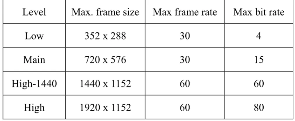
(23) Table 1.1: MPEG-2 levels: Picture size, frame-rate and bit rate constraints. 1.2.2. Level. Max. frame size. Max frame rate. Max bit rate. Low. 352 x 288. 30. 4. Main. 720 x 576. 30. 15. High-1440. 1440 x 1152. 60. 60. High. 1920 x 1152. 60. 80. Picture types. MPEG-2 contains 3 picture types, the I-picture, P-picture, and B-picture. Intra picture (I-picture) is the picture that coded without reference to other pictures. It uses the reduction of spatial redundancy to achieve compression. Because that I-picture can be decoded independently without referencing to other pictures, I-pictures can be used as the access points in the bit-stream where the decoder can start to decode. Predictive picture (P-picture) is the picture that coded by motion vectors referencing to previous I or P-pictures and residuals. It uses the reduction of temporal redundancy to achieve compression. Besides P macroblock blocks in the P-pictures, I macroblock can also exist in the P-pictures. Thus the spatial redundancy can also be reduced to achieve compression in the P-picture. P-pictures offer increased compression compared to I-pictures. Bidirectionally-predictive picture (B-picture) is similar to P-picture. Different from P-pictures, the reference frames can be either the previous picture, next picture, or both. It offers highest degree of compression.. 3.

(24) 1.2.3. Encoder/Decoder Block Diagram. The encoding process of MPEG-2 video contains the motion estimation and residual coding. Fig. 1.1 shows the simple block diagram of the MPEG-2 encoder. An embedded decoder inside the encoder calculates the result of the motion compensation so that the residual can be calculated by subtracting the input image with the motion compensated image. A Discrete-Cosine-Transform transfers the residual values to frequency-related domain. By quantizing the transferred coefficients, a Huffman run-length coder is responsible for coding the quantized coefficients and then outputting.. Input Video. -. DCT. Run-Length Coder. Quantizer Inverse Quantizer. Embedded Decoder Motion Estimation. IDCT. Motion Comp.. Frame Stores. +. Fig.1.1 A simple block diagram of MPEG-2 video encoder. Fig. 1.2 shows the simple block diagram of an MPEG-2 video decoder. A parser with Huffman run-length decoder decodes the motion vectors and quantized residual values. After inverse quantization and inverse DCT transform, the decoder calculates the residual values. By adding the motion compensated pixel values, the decoder can recover the original picture. At the time when the decoder output the decoded image, a copy of the picture must be stored into the frame buffers for the motion compensation process on next picture. The detailed decoding process will be described in section 2.1. 4.

(25) Input Bit-stream. Run-Length Decoder. Inverse Quantizer. IDCT. +. Output Video. Motion Comp.. Frame stores. Fig.1.2 A simple block diagram of MPEG-2 video decoder. 1.2.4. Bit-stream structure. Each picture is divided into several slices. Each slice is divided into several macroblocks. Each macroblock is further divided into blocks. A block is a group of 8x8 pixels, the smallest processing unit of the MPEG-2 system. Fig. 1.3 shows the hierarchical bit-stream structure of MPEG-2.. Sequence Layer. Start code. Sequence Parameter. Picture 0. Picture 1. ……. Picture N. Picture Layer. Start code. Picture flags. Slice 0. Slice 1. ……. Slice N. Slice Layer. Start code. Macroblock 1. ……. Macroblock Layer. Address. Slice address. Quantization value. Modes Block Block. Macroblock 0. …… Block. Address. Modes. Macroblock N. Motion Vectors. Block …… Block. Fig.1.3 Hierarchical bit-stream structure of MPEG-2 video. 1.3. H.264/AVC Standard Overview H.264/AVC is a standard only for videos. Its extreme low data rate is achieved by. several complex techniques and algorithms such as up to 1/4 resolution for luma and 1/8 for chroma on motion vector, several block size from 4x4 to 16x16, several modes in inter/intra prediction, CAVLC, or CABAC in context-adaptive entropy coding. 5.

(26) 1.3.1. Profiles and Levels. H.264/AVC contains 3 profiles, which are baseline, main, and extended profiles. A new profile named “high profile (Fidelity Range Extensions (FRExt))” will be included as well and is currently standardized. As Fig. 1.4 shows, I-slice, P-slice and CAVLC are the basic parts of the H.264/AVC system. CABAC and interlace is supported in main profile, and some extra slice like SP and SI slices, and data partitioning is supported in extended profile.. Main Weighted Prediction. SP and SI slices. B slices. CABAC. I slices Data partitioning. Interlace. P slices CAVLC. Extended. Slice Group and ASO Redundant slices Baseline. Fig.1.4 H.264 baseline, main, and extended profile. Much more than MPEG-2 levels can be found in the H.264 standard. From level 1 to level 5.1, max frame size ranging from 99 to 36,864 macroblocks, max video bit rate ranging from 64k to 240,000k bits/s, and motion vector ranging from +/-64 to +/-512 samples.. 6.

(27) 1.3.2. Encoder/Decoder Block Diagram. The encoding process for H.264/AVC video is more complex than the encoding process of the MPEG-2 video. Fig. 1.5 shows the simple block diagram of the H.264/AVC encoder. Same as MPEG-2 encoder, an embedded decoder exists inside the encoder that calculates the result of the motion compensation and intra prediction at the decoder side. With this embedded decoder, the encoder can foresee the decoded result and precisely calculate the residual pixel values without mismatch to the decoder. Besides inter prediction (motion compensation), intra prediction is also an important parts that tries to reduce the spatial redundancy to increase coding efficiency. Several intra prediction modes can be used for the intra predictor, and the prediction mode is decided by a mode decision block at the proceedings of the intra predictor. Not only intra prediction, the choices of the motion compensator are a lot as well. Various block sizes, multiple reference frames, short/long term prediction, and the motion vectors are all decided by motion estimation block. With these 2 strong prediction paths, the residual pixels values calculating from subtracting the input video with the prediction pixel values is closer to zero. After DCT transformation, quantization process, the entropy decoder at last reduces the coding redundancy effectively and then outputs the coded pictures.. +. Input video Motion Estimation Reference Frame Intra Mode Decision Loop Filter. -. DCT. Quanti zation. Reorder. Motion Compensation Inter prediction Intra Prediction. Embedded Decoder. Intra prediction. +. IDCT. Inverse Quant.. Fig.1.5 A simple block diagram of H.264/AVC video encoder 7. Entropy encoder. NAL.

(28) Compared with the encoder, the decoder is simpler because it lacks the decision parts like motion estimator and the intra mode decision parts. Fig. 1.6 shows a simple block diagram of the H.264/AVC video decoder. After entropy decoding the input bit-stream, the inverse quantization process and IDCT transformation transferred the bit-stream data into residual pixel values. By adding the predicted pixel values from intra predictor or motion compensator, an in-loop filter smoothed the blocking effects and then to both the output buffer and frame buffer for future reference. The details of the decoding process will be described in section 2.2.. Input bit-stream. Entropy decoder. Reorder. Inverse Quant.. IDCT. Loop Filter. +. Intra prediction Inter prediction. Output Video. Intra Prediction. Motion Compensation. Frame Buffer. Fig.1.6 A simple block diagram of H.264/AVC video decoder. 1.3.3. Bit-stream structure. Same as MPEG-2 bit-stream structure, the H.264 bit-stream is structured hierarchically, from block-level to video sequence level. Different from MPEG-2 which is the 8x8-block based system, the smallest block size in H.264/AVC system is the group of 4x4 pixels. Reference to the annex B in the H.264 standard [7], as Fig. 1.7 shows, data are all packed into NAL units. An NAL syntax element is attached in the front of each NAL unit. Each NAL unit contains an NAL unit header, which indicates the NAL unit type of the following data in this NAL unit, and the type of the RBSP (Raw Byte Sequence Payload) it contains. There’re several types of RBSP. For example, the SPS (sequence parameter set), PPS 8.

(29) (picture parameter set), and Slice layer RBSP. Slice layer RBSP includes slice header, slice data, and sometimes slice ID or redundant picture count of the partitioned slice layer. Slice data is composed of macroblocks, each consists of prediction modes (in intra macroblock) or sub-macroblock type, motion vectors (in inter macroblock) and the 4x4 block based residual data, which contributes the size of the H.264 bit-stream the most.. NAL Syntax Element. NAL Syntax Element. NAL unit. NAL Syntax Element. NAL unit. NAL unit. SPS-RBSP NAL Unit Header. NAL Syntax Element. NAL Unit Header. PPSRBSP. NAL Unit Header. Slice Layer-RBSP. Slice Header. Slice Data. Macroblock SubMacroblock Predition. ‧‧‧‧. Macroblock Macroblock Predition. Residual Data. MacroMacro‧‧‧‧‧‧ block block Residual Data. Fig. 1.7 Hierarchical structure of H.264 video bit-stream. 1.4. Thesis Organization This thesis is organized as follows. At first, the overview of the MPEG-2 and. H.264/AVC decoding flow is described in Chapter 2. Chapter 3 gives the system level design consideration and some system-level schemes in this work, like pipeline architecture, decoding ordering, system synchronization, low power mode exploration, and low power design between modules. Then, details of the architecture designs of each functional block are described in Chapter 4. Finally, the implementation details, conclusion and summary are presented in Chapter 5 and Chapter 6, respectively.. 9.

(30) 10.

(31) Chapter 2 Overview of MPEG-2 and H.264/AVC Decoding Flow The overviews of MPEG-2 decoding flow and H.264/AVC decoding flow will be given in this chapter. Though there exists some differences between the decoding flow of MPEG-2 and H.264/AVC, similarities like inverse discrete cosine transform, inverse quantization, or motion compensation can still be found. In the system point of view, to make good use of every functional block suits for both systems is an important issue and good innovation of designing a multimode video decoder.. 2.1. Overview of MPEG-2 Decoding Flow The decoding process is strictly defined in the standard. With the exception of the. Inverse Discrete Cosine Transform (IDCT) the decoding process is defined such that all decoders shall produce numerically identical results. As Fig. 1.2 shows, the decoding process mainly includes variable length decoding, inverse scanning process, inverse quantization, inverse DCT, and motion compensation.. 2.1.1. Variable length decoding. The DC coefficients are separated from other coefficients. For DC coefficients, a predictor is used for the prediction of the DC coefficients. The predictor shall be reset to a certain value at the start of a slice, a non-intra macroblock is decoded, or a macroblock is skipped. The differential value (dc_dct_differential) is coded in the bit-stream. Thus the 11.

(32) decoder can calculate the DC coefficients (QFS[0]) by. QFS[0] = dc _ dct _ pred [cc] + dct _ diff ; dc _ dct _ pred [cc] = QFS[0]; Where dc_dct_pred are the values of the 3 predictors, Y(cc=0), Cb(cc=1), and Cr(cc=2). The dct_diff is the transformed value from dc_dct_differential. For other coefficients, by table lookup of two VLC tables the values of “run” and “level” can be decoded. Then the coefficients in a macroblock can be recovered by run-length decoding process as the follows. eob_not_read = 1; while(eob_not_read){ < decode VLC, decode Escape coded coefficint if required > if( < decoded VLC indicates End of block > ){ eob_not_read = 0; while(n < 64){ QFS[n] = 0; n = n + 1; } }else{ for(m = 0; m < run; m + + ){ QFS[n] = 0; n = n + 1; } QFS[n] = signed_level n = n + 1; } }. 2.1.2. Inverse scanning process. After total 64 coefficients are decoded by the Huffman run-length VLC decoder described above, the inverse scanning process inverse scanned these coefficients to a single 8x8 block. 2 scan patterns determined by parameter “alternate_scan” can be used. Fig. 2.1 shows these 2 scan patterns.. 12.

(33) 0. 1. 5. 6. 14. 15. 27. 28. 0. 4. 6. 20. 22. 36. 38. 52. 2. 4. 7. 13. 16. 26. 29. 42. 1. 5. 7. 21. 23. 37. 39. 53. 3. 8. 12. 17. 25. 30. 41. 43. 2. 8. 19. 24. 34. 40. 50. 54. 9. 11. 18. 24. 31. 40. 44. 53. 3. 9. 18. 25. 35. 41. 51. 55. 10. 19. 23. 32. 39. 45. 52. 54. 10. 17. 26. 30. 42. 46. 56. 60. 20. 22. 33. 38. 46. 51. 55. 60. 11. 16. 27. 31. 43. 47. 57. 61. 21. 34. 37. 47. 50. 56. 59. 61. 12. 15. 28. 32. 44. 48. 58. 62. 35. 36. 48. 49. 57. 58. 62. 63. 13. 14. 29. 33. 45. 49. 59. 63. (a). (b). Fig. 2.1 Inverse scan pattern (a)alternate_scan=0 (b)alternate_scan=1. 2.1.3. Inverse quantization. As Fig. 2.2 shows, the inverse quantization process can be divided into 3 parts, the arithmetic, saturation, and mismatch control parts. In the arithmetic part, DC coefficient is separated from all the other coefficients. The parameter “intra_dc_precision” indicates the multiplication factor for DC coefficients, ranging from 1 to 8. For other coefficients, a weighting matrices W[w][v][u] and the Quant_scale_code determines the multiplication factor. W[w][v][u] can be either encoder-defined values or default values. The Quant_scale_code can be got by table lookup with the help of parameter “quantiser_scale_code” and “q_scale_type” in the bit-stream. In the saturation part, the scaled coefficients F’’[v][u] are saturated to F’[v][u] which lie in the range of [-2048:+2048]. In mismatch control, a correction is made to just one coefficient, F[7][7], adding or subtracting by one.. 13.

(34) QF[v][u]. Inverse Quantization Arithmetic. ｀＇ F [v][u]. Saturation. ｀ F [v][u]. Mismatch Control. F[v][u]. W[w][v][u] Quant_scale_code. Fig. 2.2 Inverse quantization process. In summary the inverse quantization process is any process numerically equivalent to. // Arithmetic for(v = 0; v < 8; v + 0+){ for(u = 0; u < 8; u + +){ if((u == 0) & &(v == 0) & &(macroblock_intra)){ F' '[v][u] = intra_dc_mult * QF[v][u]; }else{ if(macroblock_intra){ F' '[v][u] = (QqfF[v][u] * W[w][v][u]* quantisewr_scale * 2)/32; }else{ F' '[v][u] = (((QF[v][u] * 2) + Sign(QF[v][u])) * W[w][v][u]* quantiser_scale)/32; } } } }. 14.

(35) // Saturation sum = 0; for(v = 0; v < 8; v + + ){ for(u = 0; u < 8; u + +){ if(F' '[v][u] > 2047){ F'[v][u] = 2047; }else{ if(F' '[v][u] < -2048){ F'[v][u] = -2048; }else{ F'[v][u] = F' '[v][u]; } } sum = sum + F'[v][u]; F[v][u] = F'[v][u]; } } // Mismatch Control if((sum & 1) == 0){ if((F[7][7] & 1)!= 0){ F[7][7] = F'[7][7] - 1; }else{ F[7][7] = F'[7][7] + 1; } }. 2.1.4. Inverse Discrete-Cosine-Transform (IDCT). The formula of Inverse Discrete-Cosine-Transform is as follows:. x(m, n) = where a (0) =. 2 N. N −1 N −1. ∑∑ a(k )a(l )Y (k , l ) × cos k =0 l =0. (2n + 1)πl (2m + 1)πk × cos 2N 2N. 1 and a(k ) = 1 for k ≠ 0 2. and n,m,k,l=0,…,N-1 These transformed values shall be saturated to [-256:+255]. 15.

(36) 2.1.5. Motion compensation. As Fig. 2.3 shows, the motion compensation process includes many parts. From the bit-stream, parameters like “f_code”, “motion_code”, and “motion_residual” can be extracted. With these parameters from bit-stream, a vector decoding module with the vector predictors (PMV[r][s][t]) decodes the motion vector vector’[r][s][t] by the following process. r_size = f_code[s][t] - 1 f = 1 << r_size high = (16 * f) - 1; low = ((-16) * f); range = (32 * f); if((f == 1) || (motion_code[r][s][t] == 0)) delta = motion_code[r][s][t]; else{ delta = ((Abs(motion_code[r][s][t]) - 1) * f) + motion_residual[r][s][t] + 1; if(motion_code[r][s][t] < 0) delta = -delta; } prediction = PMV[r][s][t]; vector'[r][s][t] = prediction + delta; if(vector'[r][s][t] < low) vector'[r][s][t] = vector'[r][s][t] + range; if(vector'[r][s][t] > high) vector'[r][s][t] = vector'[r][s][t] - range; PMV[r][s][t] = vector'[r][s][t]; By scaling with a certain scaling factors, vector[r][s][t] are then sending to the address generator of frame buffers. The pixel values read from the frame buffers are then feed through a half-pel prediction filter. At the final stage, the decoded pixels is calculated by adding the combined predictions p[y][x] with the residual values f[y][x]. Saturation process is needed to clamp the result.. 16.

(37) Prediction Field/Frame Selection. Frame Buffer Addressing. Frame Buffers. vector[r][s][t] Additional Dual-Prime Arithmetic. Scaling for Color Components vector'[r][s][t]. From Bit-stream. Half-Pel Info.. Vector Decoding. Half-pel Prediction Filtering. Combine Predictions p[y][x] Vector Predictors. f[y][x]. +. Saturation. Decoded Pixels d[y][x]. Fig. 2.3 Motion compensation process. 2.2. Overview of H.264/AVC Decoding Flow The H.264/AVC decoding flow is strictly specified in the standard such that all. decoders shall produce numerically identical results. As Fig. 1.6 shows, the decoding process contains entropy decoding, reordering, inverse quantization, inverse integer discrete cosine transform, intra prediction, motion compensation, and loopfilter. In this thesis we consider the decoding process of baseline profile.. 2.2.1. Entropy decoding. The H.264 bit-stream mainly contains 2 types of contents, the parameters and the coefficients. The parameters are mainly coded by Exp-Golomb code, which is a Universal Variable Length Code (UVLC). And the coefficients of residuals are coded by Context-based Adaptive Variable Length Code (CAVLC). The entropy decoding process for Exp-Golomb code is as follows. leadingZeroBits=-1; for(b=0;!b;leadingZeroBits++) b=read_bits(1); 17.

(38) code value=2leadingZeroBits-1+read_bits(leadingZeroBits); The entropy decoding process for CAVLC is much more complicated than the decoding process of Exp-Golomb code. Many different tables are used for decoding the parameters. like. “TrailingOnes”,. “TotalCoeff”,. “level_prefix”,. “total_zeros”,. and. “run_before”. For some coefficients like “TrailingOnes” and “TotalCoeff”, more than one table are used for decoding. And the so-called “Context-based Adaptive” VLC is because that the CAVLC decoder has to choose the correct table to decode a certain parameter according to the number of coefficients in neighboring block (left and upper 4x4 blocks). By decoding the intermediate parameters like “trailing_ones_sign_flag”, “level_prefix”, “level_suffix”, “total_zeros”, and “run_before”, the run and level of this run-level code can be calculated by the procedure defined in the standard. Then a run-level code decoder is used to recover the 16 coefficients in that 4x4 block.. 2.2.2. Inverse scanning process. Input to this functional block is a list of 16 coefficients decoded by CAVLC. These 16 coefficients are then inverse scanned with a Zig-Zag scan pattern to form a 4x4 block. Fig. 2.4 shows the Zig-Zag scanning pattern.. 0. 1. 5. 6. 2. 4. 7. 12. 3. 8. 11. 13. 9. 10. 14. 15. Fig. 2.4 Zig-Zag scan. 18.

(39) 2.2.3. Inverse quantization & inverse Hadamard transform. In the inverse quantization process, the operations on DC values are separated from other coefficients. Because 4x4 block is the basic unit in H.264 systems, there are total 16 luma DC coefficients in a macroblock. These 16 DC coefficients in a macroblock are first transformed through an inverse Hadamard transform matrix as the follows 1 1 ⎤ ⎡c 00 ⎡1 1 ⎢1 1 − 1 − 1⎥ ⎢ c ⎥ ⎢ 10 f =⎢ ⎢1 − 1 − 1 1 ⎥ ⎢c 20 ⎢ ⎥⎢ ⎣1 − 1 1 − 1⎦ ⎣c30. c 01. c02. c11. c12. c 21 c31. c 22 c32. c03 ⎤ ⎡1 1 1 1⎤ ⎥ ⎢ c13 ⎥ ⎢1 1 − 1 − 1⎥ ⎥ c 23 ⎥ ⎢1 − 1 − 1 1 ⎥ ⎥⎢ ⎥ c33 ⎦ ⎣1 − 1 1 − 1⎦. The result of inverse Hadamard transformation is then scaled by the following formula with the given QPY. if QPY is greater than or equal to 12, the scaled result shall be derived as dcYij = ( fij * LevelScale(QPY %6,0,0)) << (QPY / 6 − 2) Otherwise, the scaled result shall be derived as dcYij = ( fij * LevelScale(QPY %6,0,0) + 21−QPY / 6 ) << (QPY / 6 − 2). Where ⎧v m0 for (i, j) ∈ {(0,0), (0,2), (2,0), (2,2)} ⎪ LevelScale(m, i, j ) = ⎨ v m1 for (i, j) ∈ {(1,1), (1,3), (3,1), (3,3)} , ⎪ v otherwise ⎩ m2. ⎡10 ⎢11 ⎢ ⎢13 v=⎢ 14 ⎢ ⎢16 ⎢18 ⎣. 16 13 ⎤ 18 14 ⎥⎥ 20 16 ⎥ 23 18 ⎥ ⎥ 25 20⎥ 29 23⎥⎦. For the Cb and Cr in a macroblock, the 4 DC coefficients are first transformed through a 2x2 inverse transform matrix as the follows ⎡1 1 ⎤ ⎡C 00 f =⎢ ⎥⎢ ⎣1 − 1⎦ ⎣C10. C 01 ⎤ ⎡1 1 ⎤ C11 ⎥⎦ ⎢⎣1 − 1⎥⎦. After inverse transform, scaling is performed as follows. 19.

(40) if QPY is greater than or equal to 12, the scaled result shall be derived as. dcCij = ( fij * LevelScale(QPC %6,0,0)) << (QPC / 6 − 1) Otherwise, the scaled result shall be derived as dcCij = ( fij * LevelScale(QPC %6,0,0)) >> 1 For coefficients other than DC, the scaling function is. d ij = (cij * LevelScale(qP%6, i, j )) << (qP / 6) With the given qP.. 2.2.4. Inverse Integer Discrete Cosine Transform. The Inverse Discrete Cosine Transform in H.264 system is much more simplified than the traditional Inverse Discrete Cosine Transform. The transform coefficients of 2-D IDCT in H.264 system are all simplified to integers. The transform matrix is as the follows. 1 1 ⎤ ⎡ p 00 ⎡1 1 ⎢2 1 − 1 2 ⎥ ⎢ p ⎥ ⎢ 10 cp = ⎢ ⎢1 − 1 − 1 1 ⎥ ⎢ p 20 ⎢ ⎥⎢ ⎣1 − 2 2 − 1⎦ ⎣ p30. 2.2.5. p 01. p 02. p11. p12. p 21 p31. p 22 p32. p 03 ⎤ ⎡1 2 1 1 ⎤ ⎥ ⎢ p13 ⎥ 1 1 − 1 − 2⎥ ⎢ ⎥ p 23 ⎥ ⎢1 − 1 − 1 2 ⎥ ⎥⎢ ⎥ p33 ⎦ ⎣1 − 2 1 1 ⎦. Intra prediction. The intra prediction process is a new prediction process that MPEG-2 system lacks. There are 2 classes of intra prediction modes, the Intra_4x4 prediction mode and Intra_16x16 prediction mode. There are total 9 sub-modes in Intra_4x4 prediction mode. As Fig. 2.5 shows, these 9 modes are vertical, horizontal, DC, diagonal down-left, diagonal down-right, vertical-right, horizontal-down, vertical-left, and horizontal-up, respectively. In DC modes, the intra prediction process is to calculate the mean value of neighboring pixel values. Except for DC mode, all the others are directional modes. For directional modes, the intra prediction process for the prediction values can all be written as the following formula prediction value =. (P0 + P1 + P2 + P3 ) + 2 4 20.

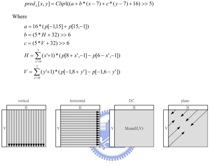
(41) Where P0, P1, P2, and P3 are all neighboring pixel values The P0, P1, P2, and P3 are different neighboring pixel values according to the type of mode and the position in the 4x4 block. For example, in mode 3 (diagonal down-left), the upper-left. corner. is. predicted. by. ((A+2B+C)+2)/4,. which. is. equivalent. to. ((A+B+B+C)+2)/4; and for upper-right corner of mode 5 (vertical-right), the prediction values is calculated by ((2C+2D)+2)/4, which is equivalent to ((C+C+D+D)+2)/4. Note that the intra prediction process and the residual adding process are processes that must be perform iteratively. That is, for a given 4x4 block, the neighboring pixel values (upper and left) for intra prediction must be residual values added.. 0 (vertical). 1 (horizontal). M A B C D E F G H. M A B C D E. I J K L. I J K L. 3 (diagonal down-left). F G H. 2 (DC) M A B C D E F G H I J Mean(A,B,C,D, K I,J,K,L) L. 4 (diagonal down-right). M A B C D E F G H I. M A B C D E I. J K L. J K L. 6 (horizontal-down). F G H. 5 (vertical-right) M A B C D E F G H I J K L. 7 (vertical-left). M A B C D E F G H I J. M A B C D E I J. K L. K L. F G H. 8 (horizontal-up) M A B C D E F G H I J K L. Fig. 2.5 Intra_4x4 prediction modes. In the intra_16x16 prediction mode class, there are total 4 modes – vertical, horizontal, DC, and plane modes respectively. The vertical mode and horizontal modes are easiest ones; the prediction is down by copying upper or left pixel values directly. In DC mode the mean value of all the upper and left neighboring pixel values has to be calculated and the result is 21.

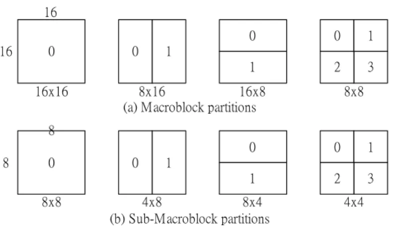
(42) assigned to all the pixels in this macroblock. The plane prediction mode is the most complex one. The formula for luma samples is given as the follows pred L [ x, y ] = Clip1((a + b * ( x − 7) + c * ( y − 7) + 16) >> 5). Where a = 16 * ( p[−1,15] + p[15,−1]) b = (5 * H + 32) >> 6 c = (5 * V + 32) >> 6 7. H = ∑ ( x'+1) * ( p[8 + x' ,−1] − p[6 − x' ,−1]) x '= 0 7. V = ∑ ( y '+1) * ( p[−1,8 + y ' ] − p[−1,6 − y ' ]) y '= 0. vertical. horizontal. H. V. DC. H. plane. H. V. V. Mean(H,V). H. V. Fig. 2.6 Intra_16x16 prediction modes. For luma samples in a macroblock, both intra_4x4 prediction modes and intra_16x16 prediction modes are valid. But for chroma samples, only the 4 modes in intra_16x16 prediction class are valid and are a little different in parameters from formula for luma samples.. 2.2.6. Motion compensation. In motion compensation process, each macroblock can be split into 4 types of partitions, 16x16, 8x16, 16x8, and 8x8. If the macroblock is split into 8x8 partitions, each 22.

(43) 8x8 partition (Sub-Macroblock) can be further split into 4 types of partitions, 8x8, 4x8, 8x4, and 4x4. This hierarchical macroblock partition gives flexibilities on motion compensation process.. 16 16. 0 16x16. 0. 0. 0. 1. 1. 2. 3. 1. 8x16 16x8 (a) Macroblock partitions. 8x8. 8 8. 0 8x8. 0. 0. 0. 1. 1. 2. 3. 1. 4x8 8x4 (b) Sub-Macroblock partitions. 4x4. Fig. 2.7 Macroblock and Sub-Macroblock partitions. The precision of motion vectors is up to 1/4. Fig. 2.8 shows an example of motion vector equals to (+1.50, -0.75).. Fig. 2.8 Up to 1/4 motion vector resolution ( mv=(+1.50, -0.75) ). The motion compensation process requires interpolation process for inter-pixel values. As Fig. 2.9 shows, for interpolating pixels with the precision of motion vector up to 1/2, a 6-tap interpolator is used for the interpolation. For example, pixel “b” is calculated by 23.

(44) b = round((E - 5F + 20G + 20H - 5I + J)/32) For interpolating pixels with the precision of motion vector up to 1/4, a 2-tap interpolator is used for the interpolation. For example, pixel “n” is calculated by n = round((c + f)/2). A a B C b D G E d K. F e L. G c H f g h M k N. I i P. J j Q. c H n s p f t g u h q v r M k N. R l S T m U Fig. 2.9 Interpolation for pixel values. The motion vector MV is calculated by adding the MVD (motion vector difference) with the MVP (motion vector prediction). The MVD is decoded from the bit-stream. MVP is calculated from the motion vectors of neighboring blocks.. 2.2.7. De-blocking filter. Same as MPEG-2, H.264/AVC system is block-based video coding system. Though we can perform discrete cosine transform to take advantage of the spatial correlation property and exploit motion compensated prediction to improve the compression ratio on the block-based systems, the disadvantage of the block-based system lies on the discontinuity on each block boundaries which is also known as blocking effects because of the quantization loss that annoying the continuity on block boundaries. Moreover, the blocking-effect propagated from frame to frame due to the motion compensation. Thus, a de-blocking filter is demanded and is included in the H.264 standard as an in-loop filter. 24.

(45) As Fig. 2.10 shows, the edge filtering order defined in the standard is a, b, c, d, e, f, g, then h. For a given 4x4 blocks, as long as the filter ordering to this 4x4 block is left, right, upper, and down, is standard compliant.. e f g h a. b. c. d. Fig. 2.10 Edge filtering order in a macroblock. The filtering process to a certain boundary is through an interpolator. Each filtering operation can at most changes 3 pixel values either in both sides of the boundary. The choice of filtering outcome depends on the boundary strength and on the gradient of image samples across the boundary. The boundary strength bS is in the range of 0 to 4, from no filtering to strongest filtering according to the quantiser, coding modes of neighboring blocks and the gradient of image samples.. p3 p2 p1 p0 p3. p2. p1. p0. q0. q1. q2. q3. q0 q1 q2 q3. Fig. 2.11 Adjacent pixels to horizontal and vertical boundaries 25.

(46) 26.

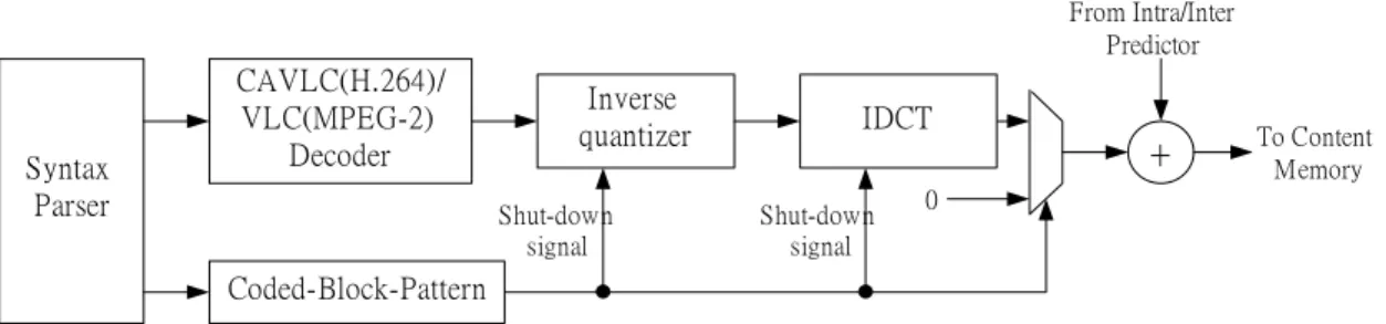
(47) Chapter 3 System Design Of MPEG-2 and H.264/AVC Decoder In this chapter, we show some design techniques like pipeline scheme, synchronization problem and solution, decoding ordering, and power saving techniques from the system point of view.. 3.1. MPEG-2 and H.264/AVC Combined System Decoding Flow Fig. 3.1 shows our MPEG-2/H.264 combined decoder diagram. Input to this decoder is. the video bit-stream and a video type signals. This video type signal acknowledges the decoder the type of the video bit-stream is feeding. For H.264 video bit-stream, an H.264 syntax parser is firstly syntax analyzed the bit-stream, stored the system parameter into system-wide shared registers, send the bit-stream to the following residual path (CAVLC, 4x4-scaling, 4x4 IDCT) or prediction path (H.264 Intra predictor, H.264 Motion Compensator), summed them together with the help of synchronizer, a loopfilter process the summed pixel value and then output it both to frame buffer or to the display. For MPEG-2 video bit-stream, same as the H.264 decoding flow, first, a MPEG-2 syntax parser analyzed the bit-stream, stored the system parameter into system-wide shared registers, send the bit-stream to the following MPEG-2 VLC decoder, 8x8 inverse quantizer, 8x8 IDCT, MPEG-2 Motion Compensator, and an optional MPEG-2 post filter is at the end 27.

(48) of the decoding flow. For the hardware sharing issues, we share the registers in syntax parsers, design a CAVLC/VLC combined decoder for entropy decoding, a H.264/MPEG-2 combined motion compensator, a synchronizer for both system, content memory and frame buffer for both systems, and the de-blocking filter for both system which functions as an in-loop filter for H.264 system and a post-processing filter for MPEG-2 system.. Off chip Frame Buffer Single port Mx8. N : Frame Width M : Frame Size H264 Decoder. Combined Syntax Parser Video type. Video Bit-stream. 8x8 InverseQuantization. H.264 Syntax Parser Shared Regs MPEG2 Syntax Parser. BUS. H.264/MPEG2 Combined Motion Compensator. 8x8 IDCT Single port (Nx2/4)x32. H.264 Intra predictor. Residual Adder. DC coeff. CAVLC(H.264) / VLC (MPEG2) Combined Decoder. 4x4 Scaling Unfiltered Pixel values. 4x4 IDCT / Hadamard. +. Synchr onizer. Single port 96x32 Single port 96x32. Single port (Nx2)x32. H.264 LoopFilter / MPEG2 Post Filter. Filtered Pixel values (Normal Mode). Frame output. (Low Power Mode). Fig. 3.1 MPEG-2/H.264 Combined Decoder Diagram. 3.2. Hybrid 4x4-Block Level Pipeline with Instantaneous Switching Scheme for H.264/AVC Decoder. 3.2.1. Hybrid 4x4-Block Level Pipeline Architecture. The 4x4 block is the smallest group of pixels that the H.264/AVC standard adopts. We can see from the standard that a 4x4 Inverse-Discrete-Cosine-Transform (IDCT), a 4x4-block based inverse scanning process, and a 4x4 inverse quantization matrix for 28.

(49) rescaling, are required in decoding H.264/AVC video sequence. Moreover, the smallest intra prediction unit is 4x4 sized block, and so do the motion compensation process. Thus in our H.264/AVC decoder design, compared with conventional macroblock-level pipelining architecture [1] [6], our 4x4-block level pipelining architecture are more suitable for the 4x4-block based H.264/AVC system. Compared with macroblock-level (16x16) and block-level (8x8) pipeline parallelism, a trade-off exists between processing cycles and buffer cost. For the processing cycles issue, refers to Fig.3.2, we can see that the 4x4-sub-block-level pipeline parallelism requires more additional processing cycle than cycles needed of macroblock-level pipeline parallelism. Although this penalty has to be paid by the 4x4-sub-block-level pipeline parallelism, the cost saved of the buffer storage required is worthy.. 15. 15. 15. i =0. i =0. i =0. ∑ max( pi , qi ) ≥ max(∑ pi , ∑ qi ) Macroblock i 4x4-Sub-Block-Level Pipeline Parallelism. Stage 1. 15. 0. 1. 2. 3. 4. 5. 6. 7. 8. 9. 10. 11. 9. 10. 12. 13 14. 15. 0. 1. 2. Macroblock i Stage 2. 14 15. 0. 1. 2. 3. 4. 5. 6. 7. 8. 11. 12. 13 14. 15. 0. 1. Processing Cycle Difference. Macroblock i Macroblock-Level Pipeline Parallelism. Stage 1 15. 0. 1. 2. 3. 4. 5. 6. 7. 8. Macroblock i+1 9. 10. 11. 12. 13 14 15. 0. 1. Macroblock i-1 Stage 2. 14 15 0. 1. 2. 3. 4. 5. 6. 7. 8. 9. 10 11 12 13. 2. 3. 4. 5. Macroblock i 14 15. 0. 1. 2. 3. 4. Fig.3.2 Additional processing cycles required for 4x4-sub-block-level pipeline parallelism. Compared with macroblock-level (16x16) and block-level (8x8) pipeline parallelism, because the processing unit of data in each stage is quite smaller (4x4) in 4x4-sub-block-level pipeline parallelism that the only 4x4-sub-block-level sized buffer storage is enough. We can see from Table 3.1, three different parallelisms show the trade-off between buffer cost and processing cycles. For 4x4-sub-block-level pipeline parallelism, 29.

(50) although 1.26 times processing cycles required compared with macroblock-level pipeline parallelism, 15/16 buffer storage can be saved.. Table3.1: Trade-off between processing cycles and buffer cost Parallelism. Unit of Data. Buffer Cost. Processing Cycles. Macroblock-Level. 16x16. X16. M cycles/MB. Block-Level. 8x8. X4. 1.19*M cycles/MB. Sub-Block-Level. 4x4. X1. 1.26*M cycles/MB. Moreover, besides the saving in storage cost, the large amount of power induced by these buffers which are active all the time could be greatly reduced as well. As Table 3.3 shows, the 4x4-sub-block-level sized storage buffers in CAVLC & IDCT consume 1.453mW and 0.864mW under clock frequency 100MHz, which contribute 2.86% of total power (81.072mW) when summed together. But if the macroblock-level sized buffers are used instead, the power of these storage buffers would be 23.251mW and 13.824mW, which is 15 times greater than the case of 4x4-sub-block-level pipeline parallelism.. Table 3.3 Power dissipated by buffers between pipeline stages Storage buffer in CAVLC. Storage buffer in IDCT. Parallelism Num. of regs. Power. Num. of regs. Power. Macroblock-Level. 16x16x8 (bits). 23.251 mW. 16x16x18 (bits). 13.824 mW. Block-Level. 8x8x8 (bits). 5.813 mW. 8x8x18 (bits). 3.456 mW. Sub-Block-Level. 4x4x8 (bits). 1.453 mW. 4x4x18 (bits). 0.864 mW. 30.

(51) Although we saves the cost of storage buffer and the associated power reduction by adopting 4x4-sub-block-level pipeline parallelism, this 4x4-sub-block-level pipeline parallelism can’t be applied on some other modules which also exist in the decoding flow like motion compensator and loopfilter because of their macroblock-level-characteristic. Motion compensator must supports inter prediction process for several block sizes, from 4x4, 4x8, 8x4, 8x8, 16x8, 8x16, to 16x16. It is hard to divide the inter prediction process for block sized modes other than 4x4-block-sized mode into several 4x4-sub-block-sized inter prediction processes. So we choose to maintain traditional macroblock-level pipeline parallelism on motion compensation stage. For in-loop filtering operation, i.e. loopfilter, it is also hard to be divided into several identical 4x4-sub-block filtering process because the neighboring 4x4-sub-blocks it has to fetch is irregular according to inverse scanning sequence. In contrary, the filtering process is almost identical in macroblock level. Thus we also choose macroblock-level pipeline parallelism for loopfilter. In our overall pipeline design, we combine the 4x4-sub-block-level pipeline parallelism with macroblock-level pipeline parallelism to a hybrid pipeline scheme that suits best for each module. The pipeline parallelism applied for decoding modules is summarized in Table 3.4.. 31.

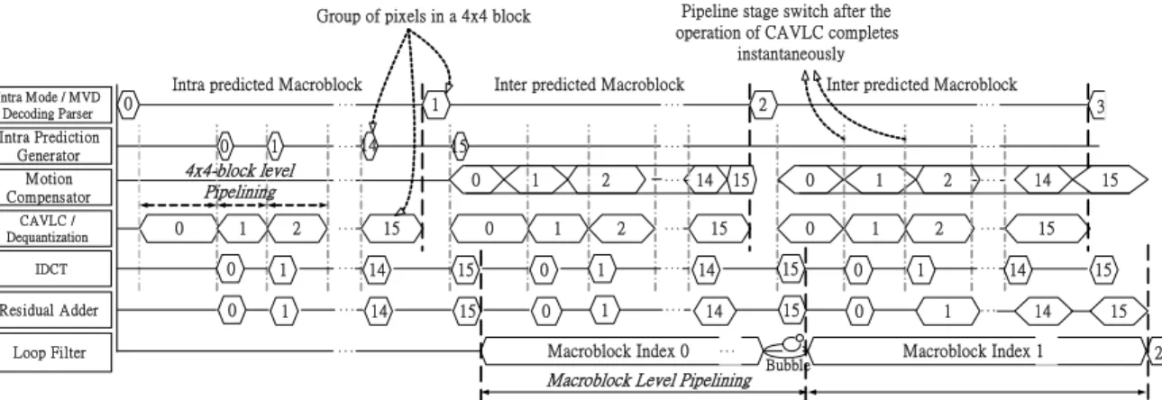
(52) Table 3.4 Summary of pipeline parallelism applied. 3.2.2. Module. Pipeline parallelism. Intra predictor. 4x4-sub-block-level. CAVLC. 4x4-sub-block-level. De-quantizer. 4x4-sub-block-level. IDCT. 4x4-sub-block-level. Motion compensator. Macroblock-level. Loopfilter. Macroblock-level. Instantaneous Switching Scheme. We also applied an instantaneous switching scheme in our 4x4-sub-block-level pipeline design, that is, we switch our pipeline stage as soon as possible. As long as all pipelined modules complete their work, we switch the pipeline into next stage instantaneously. Because of this instantaneous switching scheme we applied, any pipelined module with especially long processing cycles would be the bottleneck of the whole decoding system. The pipeline stage must be switched only if all the pipelined modules complete their work. So all the other pipelined modules must be idle and wait for the pipelined module with especially long processing cycles if exists, bubbles induced in this kind of situation would be a lot that degrades overall system throughput much. Thus, we try to balance the cycle count required for each modules, so that the idle time of these pipelined modules like CAVLC, De-quantization, IDCT, and etc could be minimized that this instantaneous switching scheme can be a great help of maximizing our system throughput. Fig. 3.3 shows an example pipelining schedule of hybrid 4x4-sub-block-level pipeline parallelism with instantaneous switching scheme. 32.

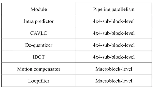
(53) Pipeline stage switch after the operation of CAVLC completes instantaneously. Group of pixels in a 4x4 block. Intra M ode / MVD Decoding Parser. Intra predicted Macroblock 0. Intra Prediction Generator. 0. 1. ‧‧‧. 4x4-block level Pipelining. M otion Compensator CAVLC / Dequantization. 0. 1. 2. IDCT. 0. 1. Residual Adder. 0. 1. Loop Filter. Inter predicted Macroblock 1. ‧‧‧. 14. 15. ‧‧‧. ‧‧‧. ‧‧‧. ‧‧‧. 15. 1. 2. 0. 1. ‧‧‧. 2. 14. 15. 0. 1. 14. 15. 0. 1. ‧‧‧. ‧‧‧. ‧‧‧. Macroblock Index 0. 3. ‧‧‧. ‧‧‧. 0. ‧‧‧. Inter predicted Macroblock 2. ‧‧‧. ‧‧‧. 14. 15. 15 14 14. 0. 1. 0. 1. 15. 0. 15. 0. ‧‧‧. Macroblock Level Pipelining. Bubble. 2 2. 14. ‧‧‧. 15. ‧‧‧. 1. ‧‧‧. 1. ‧‧‧. 15. 14. 15 14. 15. Macroblock Index 1. 2. Fig. 3.3 An example of the pipelining schedule. 3.3. Efficient 1x4 Column-By-Column Decoding Ordering Based on our proposed 4x4-sub-block-level pipeline parallelism, we choose 4 pixels. per cycle as our overall system throughput. The throughput of 4 pixels per cycle is also very suitable for the efficient IDCT design, inverse quantizer design, and inter/intra predictor design. Limited by the 4x4-sub-block inverse scanning sequence (also the decoding sequence) defined by H.264/AVC standard, we have two choices on the decoding ordering that are both standard compliant, the 4x1 row-by-row decoding ordering and the 1x4 column-by-column decoding ordering, as Fig. 3.4 and Fig. 3.5 shows respectively. After the analysis for inter and intra predictor on these 2 types of decoding order given in the following, we will see that the 1x4 column-by-column decoding ordering is better than 4x1 row-by-row decoding ordering both in fewer memory access times and fewer decoding cycles.. 33.

(54) 20 21 22 23 28 29 30 31 52 53 54 55 60 61 62 63. 16 17 18 19 24 25 26 27 48 49 50 51 56 57 58 59. 4 5 6 7 12 13 14 15 36 37 38 39 44 45 46 47. 0 1 2 3 8 9 10 11 32 33 34 35 40 41 42 43. Fig. 3.4 4x1 row-by-row decoding ordering. 0. 1. 2. 3. 4. 5. 6. 7. 1 6. 1 7. 1 8. 1 9. 2 0. 2 1. 2 2. 2 3. 8. 9. 1 0. 1 1. 1 2. 1 3. 1 4. 1 5. 2 4. 2 5. 2 6. 2 7. 2 8. 2 9. 3 0. 3 1. 3 2. 3 3. 3 4. 3 5. 3 6. 3 7. 3 8. 3 9. 4 8. 4 9. 5 0. 5 1. 5 2. 5 3. 5 4. 5 5. 4 0. 4 1. 4 2. 4 3. 4 4. 4 5. 4 6. 4 7. 5 6. 5 7. 5 8. 5 9. 6 0. 6 1. 6 2. 6 3. Fig. 3.5 1x4 column-by-column decoding ordering. Now we give an analysis for both inter and intra prediction units on these 2 decoding ordering.. 3.3.1. Analysis on inter prediction unit. In our inter predictor design also known as motion compensator, an initialization stage is required before any contiguous output of motion compensated pixel values. The 34.

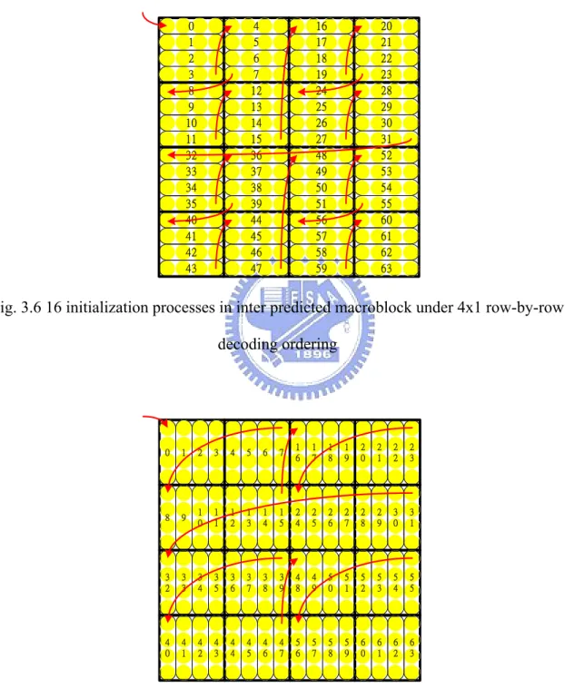
(55) initialization period requires 18 memory access times for loading related neighboring 9*6=54 pixel values from the reference frame for the 2-D interpolation (6-tap interpolation then 2-tap interpolation) of the target pixel values. 18 cycles (9 pixels per 3 cycles) also required for this operation in the initialization stage. After the initialization stage is finished for the 1st group of 4 motion compensated pixel values, the loaded pixel values in the initialization stage can be reused and only 9 new pixels are needed to be loaded for computing the following contiguous output. This computing process requires only 3 memory access times and 3 cycles for the following contiguous outputs of a group of 4 motion compensated pixel values. For decoding an inter predicted macroblock under 4x1 row-by-row decoding ordering and 1x4 column-by-column decoding ordering, we can found that as Fig. 3.6 shows, for the 4x1 row-by-row decoding ordering, there exists 16 discontinuities (3rd, 7th, 11th, 15th, 19th, 23rd, 27th, 31st, 35th, 39th, 43rd, 47th, 51st, 55th, 59th and 63rd outputs) in decoding ordering. Each discontinuity output of a group of 4 pixel values requires an initialization process. 3 contiguous outputs are then followed by each discontinuous output. Thus for 4x1 row-by-row decoding ordering, total memory access times and total decoding cycles are 16x18 (discontinuous output) + 16x3x3 (contiguous output) = 432 memory access (3.1) 16x18 (discontinuous output) + 16x3x3 (contiguous output) = 432 cycles. (3.2). As Fig. 3.7 shows, for 1x4-column-by-column decoding ordering, only 8 discontinuities (7th, 15th, 23rd, 31st, 39th, 47th, 55th and 63rd outputs) exist in decoding ordering, which leads to 8 initialization process for these 8 outputs. 7 contiguous outputs are then followed by each discontinuous output. Thus for 1x4-column-by-column decoding ordering, total memory access times and total decoding cycles are 8x18 (discontinuous output) + 8x7x3 (contiguous output) = 312 memory access (3. 3) 8x18 (discontinuous output) + 8x7x3 (contiguous output) = 312 cycles 35. (3.4).

(56) In summary, for an inter predicted macroblock, the memory access times and decoding cycles saved by adopting 1x4-column-by-column decoding ordering instead of 4x1-row-by-row decoding ordering are both 28%.. 20 21 22 23 28 29 30 31 52 53 54 55 60 61 62 63. 16 17 18 19 24 25 26 27 48 49 50 51 56 57 58 59. 4 5 6 7 12 13 14 15 36 37 38 39 44 45 46 47. 0 1 2 3 8 9 10 11 32 33 34 35 40 41 42 43. Fig. 3.6 16 initialization processes in inter predicted macroblock under 4x1 row-by-row decoding ordering. 0. 1. 2. 3. 4. 5. 6. 7. 1 6. 1 7. 1 8. 1 9. 2 0. 2 1. 2 2. 2 3. 8. 9. 1 0. 1 1. 1 2. 1 3. 1 4. 1 5. 2 4. 2 5. 2 6. 2 7. 2 8. 2 9. 3 0. 3 1. 3 2. 3 3. 3 4. 3 5. 3 6. 3 7. 3 8. 3 9. 4 8. 4 9. 5 0. 5 1. 5 2. 5 3. 5 4. 5 5. 4 0. 4 1. 4 2. 4 3. 4 4. 4 5. 4 6. 4 7. 5 6. 5 7. 5 8. 5 9. 6 0. 6 1. 6 2. 6 3. Fig. 3.7 8 content switches in inter predicted macroblock under 1x4 column-by-column decoding ordering. 36.

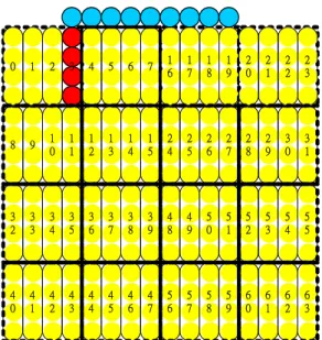
(57) 3.3.2. Analysis on intra prediction unit. Based on the H.264/AVC standard, for an Intra4x4 predicted macroblock, the neighboring pixels including upper 8 pixels, left 4 pixels plus a corner pixel (total 13 pixels) must be loaded before the intra prediction process. Because we follow this rule in our intra predictor design, accessing from memory for these 13 pixels are required before each intra4x4 prediction process no matter which prediction mode is for this 4x4-sub-block. We found that if we choose the 1x4 column-by-column decoding ordering as Fig. 3.5 show, a group of 4 pixels of every 4th output is just the left 4 neighboring pixels that originally required to be fetched from neighbor for intra prediction on next 4x4-block. For example, as Fig. 3.8 shows, the group of 4 pixels in the 3rd output is just the left 4-neighboring pixels to be fetched for the following 4x4-sub-block. In this way, this group of 4 pixels can be forwarded directly from previous output instead of fetching from memory that reduces the memory access times. Same situation also occurs at the 11th, 19th, 27th, 35th, 43rd, 51st, 59th outputs too. However, for 4x1-row-by-row decoding ordering, this property can not be found to reduce the memory access times. In summary, the memory access times can be reduced from 3x16=48 times to 3x8+2x8=40 times (17% saved) by adopting 1x4-column-by-column decoding ordering instead of 4x1-row-by-row decoding ordering.. 37.

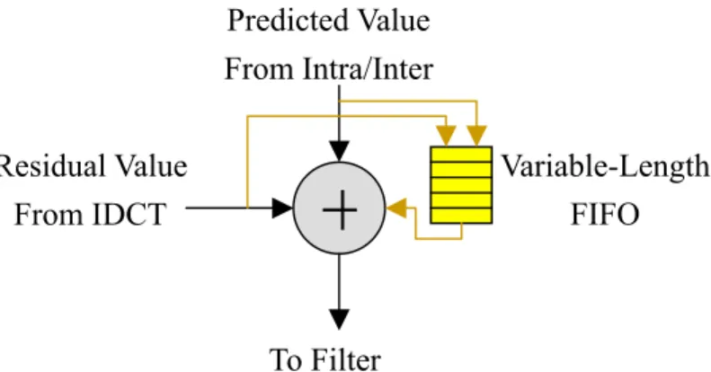
(58) 0. 1. 2. 3. 4. 5. 6. 7. 1 6. 1 7. 1 8. 1 9. 2 0. 2 1. 2 2. 2 3. 8. 9. 1 0. 1 1. 1 2. 1 3. 1 4. 1 5. 2 4. 2 5. 2 6. 2 7. 2 8. 2 9. 3 0. 3 1. 3 2. 3 3. 3 4. 3 5. 3 6. 3 7. 3 8. 3 9. 4 8. 4 9. 5 0. 5 1. 5 2. 5 3. 5 4. 5 5. 4 0. 4 1. 4 2. 4 3. 4 4. 4 5. 4 6. 4 7. 5 6. 5 7. 5 8. 5 9. 6 0. 6 1. 6 2. 6 3. Fig. 3.8 Reduction on memory access of the intra predicted macroblock. 3.4. Prediction/Residual Synchronization Scheme In both H.264/AVC and MPEG2 decoder designs, there exist 2 decoding paths, say,. inter/intra prediction path (prediction path) and residual recovery path (residual path). The prediction path predicted the pixel values from the motion vector by motion compensator or by intra prediction mode by intra predictor. The residual path decodes the residual pixel values first by entropy decoding the coded data by CAVLC/CABAC (H.264/AVC) or table based VLC (MPEG2). A de-quantization process is then performed on the decoded value. Finally, an inverse discrete-cosine-transform (IDCT) transfers the scaled values into residual values and output them at the end of the residual path. The decoder has to add the predicted pixel values from prediction path with the residual pixel values from residual path to reconstruct the original picture before an in-loop filter (H.264/AVC) or a post-filter (MPEG2). The synchronization problem exists in this adder that adds the pixel values come from 2 different decoding paths. Because the output timing of these 2 paths is different, we can not guarantee the output timing of the pixel values come from 2 paths is simultaneous in a 38.