整數階與分數階帶離心調速器之旋轉機械系統的渾沌同步與渾沌激發之超渾沌

全文

(1)國立交通大學機械工程學系碩士論文. 整數階與分數階帶離心調速器之旋轉機械系統的渾沌同步與渾沌激發之超渾沌. Chaos Synchronization and Chaos-Excited Hyperchaos, for Integral and Fractional Order Rotational Machine System with Centrifugal Governor. 研究生：莊為任指導教授：戈正銘. 教授. 中華民國九十四年六月.

(2) 整數階與分數階帶離心調速器之旋轉機械系統的渾沌同步與渾沌激發之超渾沌. Chaos Synchronization and Chaos-Excited Hyperchaos, for Integral and Fractional Order Rotational Machine System with Centrifugal Governor. 研究生：莊為任指導教授：戈正銘. Student：Wei-Ren Jhuang Advisor：Zheng-Ming Ge. 國. 立. 交. 通. 大. 學. 機. 械. 工. 程. 學. 系. 碩士論文. A Thesis Submitted to Department of Mechanical Engineering College of Engineering National Chiao Tung University In Partial Fulfillment of the Requirements For the Degree of Master of Science In Mechanical Engineering June 2005 Hsinchu, Taiwan, Republic of China 中華民國九十四年六月.

(3) 整數階與分數階帶離心調速器之旋轉機械系統的渾沌同步與渾沌激發之超渾沌. 學生：莊為任. 指導教授：戈正銘. 國立交通大學機械工程研究所碩士班. 摘. 要. 本篇論文研究整數階與分數階帶離心式調速器之旋轉機器系統的渾沌同步與渾沌激發之超渾沌。透過數值分析，如相圖，分叉圖，和Lyapunov指數，可以觀察到週期與渾沌運動。利用線性回饋控制與適應性控制，使得整數階系統達成渾沌同步。接著,提出一個新的概念：透過渾沌系統之狀態驅動的渾沌取代透過正弦時間函數驅動的渾沌。此研究乃一個完全新的領域，觀察到超渾沌與廣範圍的渾沌。最後，發現分數階系統的階數少於或多於原系統的狀態數目時皆存在渾沌現象。利用類似於用在整數階系統的方法，系統可以達成渾沌控制與渾沌同步。.

(4) Chaos Synchronization and Chaos-Excited Hyperchaos, for Integral and Fractional Order Rotational Machine System with Centrifugal Governor Student：Wei-Ren Jhuang. Advisor：Zheng-Ming Ge. Department of Mechanical Engineering National Chiao Tung University. ABSTRACT Chaos synchronization and chaos-excited hyperchaos, for integral and fractional order rotational machine system with centrifugal governor are studied in this thesis. By applying numerical analysis such as phase portrait, bifurcation diagram and Lyapunov exponent, periodic and chaotic motions are observed. Chaos synchronization for integral order system is accomplished by employing both linear feedback control and adaptive control based on Lyapunov first approximation theorem and asymptotical stability theorem. Then a new concept of chaos driven by states of chaotic system instead of driven by sinusoidal time function is put forward. This research is a completely new field, hyperchaos and broader ranges of chaos are obtained. Finally, it is found that chaos exists in the fractional order system with order less and more than number of states of the system. By utilizing the similar scheme as that for their integral order correspondence, chaos control and chaos synchronization are accomplished.. i.

(5) ACKNOWLEDGMENT. 此篇論文及碩士學業之完成，首先，必須感謝指導教授戈正銘老師的敦敦教誨。老師因才施教的教學方式，在他的殷殷教導之下，使我能在研究的生活中怡然而自得。老師最令我欽佩的是對學術與詩詞文學所投注的那份熱情。此外，老師虛懷若谷與幽默樂觀的處世態度，更是我效法的楷模。短短的兩年碩士生涯，感謝我的兩位同學，林國樺與楊坤偉，感謝他們在學業與生活上的鼎力相助。在研究陷入渾沌的困境時，感謝李青一、鄭普建與陳炎生等諸位學長的熱心指導，幫助我走出渾沌的崎嶇道路。此外，也感謝其他同學陪我渡過這段日子。最重要的是要感謝父母的支持，讓我毫無羈絆的完成學業。回想 18 年來求學的日子，父母的撫養、老師的教導以及朋友們的砥礪，將是我未來事業衝刺的動力。. ii.

(6) CONTENTS ABSTRACT ...............................................................................................................................i ACKNOWLEDGMENT ..........................................................................................................ii CONTENTS .............................................................................................................................iii LIST OF FIGURES ..................................................................................................................v Chapter 1. Introduction .........................................................................................................1. Chapter 2 Regular and Chaotic Dynamics of Rotational Machine System with Centrifugal Governor .................................................................................3 2.1 Autonomous System. 3. 2.2 Nonautonomous System. 5. Chapter 3 Chaos Synchronization by Linear Feedback Control and Adaptive Control ..........................................................................................7 3.1 Chaos Synchronization by Linear Feedback Control 3.2 Chaos Synchronization by Adaptive Control. Chapter 4. 7 10. Hyperchaos Excited by Chaos for Rotational Machine System with Centrifugal Governor ...............................................................................12. 4.1 Chaos Excited by Single Autonomous Chaos. 12. 4.2 Chaos Excited by Single Nonautonomous Chaos. 16. Chapter 5 Chaos, Its Control and Synchronization of Fractional Order Chaotic System...................................................................................................18 5.1 Review of Fractional Operator. 18. iii.

(7) 5.2 The Fractional Order Autonomous Chaotic System. 19. 5.2.1 Chaos Control. 19. 5.2.2. Chaos Synchronization of the Same Fractional Order systems. 20. 5.2.3. Chaos Synchronization of Different Fractional Order systems. 21. 5.3 The Fractional Order Nonautonomous Chaotic System. 21. 5.3.1 Chaos Control. 22. 5.3.2. Chaos Synchronization of the Same Dractional Order Systems. 23. 5.3.3. Chaos Synchronization of Different Fractional Order Systems. 23. Chapter 6 Conclusions.........................................................................................................25. REFERENCES .......................................................................................................................73. iv.

(8) LIST OF FIGURES Fig. 2.1.1. Physical model of a rotational machine with a fly-ball governor system.. 26. Fig. 2.1.2. Three Lyapunov exponents for k between 1.942 and 20.. 27. Fig. 2.1.3. (a) Phase portrait (b) Poincaré map for k = 2.603 .. 28. Fig. 2.2.1. Three Lyapunov exponents for k between 1.942 and 20.. 29. Fig. 2.2.2. (a) Phase portrait (b) Poincaré map for k = 17.8 .. 30. Fig. 2.2.3. Projection of Poincaré map of: (a) quasi-periodic (b) chaotic motion on x − y plane.. 31. Fig. 3.1. Time history of errors for g x = 0.059 , g z = 2.21 .. 32. Fig. 3.2. Time history of errors for g x = 0.059 , θ = 1 .. 32. Fig. 4.1.1. Three Lyapunov exponents for k between 2 and 10, f (t ) = 0.2 x .. 33. Fig. 4.1.2. Three Lyapunov exponents for k between 2 and 15, f (t ) = −0.2 x .. 33. Fig. 4.1.3. Three Lyapunov exponents for k between 2 and 10, f (t ) = 0.2 y .. 34. Fig. 4.1.4. Three Lyapunov exponents for k between 2 and 15, f (t ) = −0.2 y .. 34. Fig. 4.1.5. Three Lyapunov exponents for k between 2 and 15, f (t ) = −0.4 y .. 35. Fig. 4.1.6. Three Lyapunov exponents for k between 2 and 10, f (t ) = 0.1z .. 36. Fig. 4.1.7. Three Lyapunov exponents for k between 2 and 15, g (t ) = 0.2 x .. 37. Fig. 4.1.8. Three Lyapunov exponents for k between 2 and 10, g (t ) = −0.1x .. 37. Fig. 4.1.9. Three Lyapunov exponents for k between 2 and 8, g (t ) = −0.2 x .. 38. Fig. 4.1.10 Three Lyapunov exponents for k between 2 and 10, g (t ) = 0.1y .. 38. Fig. 4.1.11 Three Lyapunov exponents for k between 2 and 10, g (t ) = 0.2 y .. 39. Fig. 4.1.12 Three Lyapunov exponents for k between 2 and 10, g (t ) = 0.4 y .. 39. Fig. 4.1.13 Three Lyapunov exponents for k between 2 and 12, g (t ) = −0.05 z .. 40. Fig. 4.1.14 Three Lyapunov exponents for k between 2 and 12, g (t ) = −0.1z .. 40. Fig. 4.1.15 Three Lyapunov exponents for k between 2 and 12, h(t ) = 0.2 x .. 41. Fig. 4.1.16 Three Lyapunov exponents for k between 2 and 10, h(t ) = −0.8 ~ 1y (t ) .. 42. Fig. 4.1.17 Three Lyapunov exponents for k between 2 and 12, h(t ) = 0.2 z .. 43. Fig. 4.2.1. Three Lyapunov exponents for k between 2 and 10, f (t ) = −0.2 x .. Fig. 4.2.2. Three Lyapunov exponents for k between 2 and 15, (a) f (t ) = 0.4 y. (b) f (t ) = −0.4 y .. v. 44. 45.

(9) Fig. 4.2.3. Three Lyapunov exponents for k between 2 and 8, f (t ) = 0.1z .. 46. Fig. 4.2.4. Three Lyapunov exponents for k between 2 and 10, g (t ) = 0.6 y .. 47. Fig. 4.2.5. Three Lyapunov exponents for k between 2 and 10, g (t ) = −0.6 y .. 48. Fig. 4.2.6. Three Lyapunov exponents for k between 2 and 6.5, h(t ) = −0.2 x .. 49. Fig. 4.2.7. Three Lyapunov exponents for k between 2 and 8, h(t ) = 0.2 z .. 50. Fig. 5.2.1. Phase portrait of the fractional order autonomous system with order q = 0.9.. Fig. 5.2.2. 51. Phase portrait of the fractional order autonomous system with order q = 1.1.. Fig. 5.2.3. 52. Bifurcation diagram of the fractional order autonomous system with order q = 0.9.. Fig. 5.2.4. 53. Bifurcation diagram of the fractional order autonomous system with order q = 1.1.. Fig. 5.2.5. 54. Time history of the state variables of the controlled integral order autonomous system with order q = 1.. Fig. 5.2.6. Time history of the state variables of the controlled fractional order autonomous system with order q = 0.9.. Fig. 5.2.7. 57. Time history of errors of the fractional order autonomous system with order q = 0.9.. Fig. 5.2.9. 56. Time history of the state variables of the controlled fractional order autonomous system with order q = 1.1.. Fig. 5.2.8. 55. 58. Time history of errors of the fractional order autonomous system with order q = 1.1.. 59. Fig. 5.2.10 Time history of errors of different fractional order autonomous systems with order q = 0.9 and p = 1.1.. 60. Fig. 5.2.11 Time history of errors of different fractional order autonomous systems with order q = 1.1 and p = 0.9. Fig. 5.3.1. 61. Phase portrait of the fractional order nonautonomous system with order q = 0.9.. Fig. 5.3.2. 62. Phase portrait of the fractional order nonautonomous system with order q = 1.1.. Fig. 5.3.3. 63. Bifurcation diagram of the fractional order nonautonomous system vi.

(10) with order q = 0.9. Fig. 5.3.4. 64. Bifurcation diagram of the fractional order nonautonomous system with order q = 1.1.. Fig. 5.3.5. 65. Time history of the state variables of the controlled integral order nonautonomous system with order q = 1.. Fig. 5.3.6. Time history of the state variables of the controlled fractional order nonautonomous system with order q = 0.9.. Fig. 5.3.7. 68. Time history of errors of the fractional order nonautonomous system with order q = 0.9.. Fig. 5.3.9. 67. Time history of the state variables of the controlled fractional order nonautonomous system with order q = 1.1.. Fig. 5.3.8. 66. 69. Time history of errors of the fractional order nonautonomous system with order q = 1.1.. 70. Fig. 5.3.10 Time history of errors of different fractional order nonautonomous systems with order q = 0.9 and p = 1.1.. 71. Fig. 5.3.11 Time history of errors of different fractional order nonautonomous systems with order q = 1.1 and p = 0.9.. 72. vii.

(11) Chapter 1 Introduction. It goes without doubt that chaos synchronization has been the important issues in the recent years [1-9]. A lot of researches have shown that chaotic phenomena are observed in many physical systems that possess nonlinearity [10-12]. Chaotic motions also occur in many nonlinear control systems [13-14]. Chaotic phenomena are quite useful in many applications such as human brain [15-16], optical communication [17-20], heart rate variability [21-22], etc. Chaos synchronization has been applied in many fields such as secure communication [23-28], chemical and biological systems, etc. Most of physical systems in nature are nonlinear and can be described by the nonlinear equations of motion which in general can not be linearized. Hence the studies of nonlinear systems spread quickly today. For the nonlinear system, the study of the types of system behavior, the effects to the behavior caused by different parameters and initial conditions, the behavior analysis of the system, consist of the major tasks. Besides, we are also interested in the understanding of the complicated phenomena arose from nonlinearity. The central characteristics are that a process like randomization happens in the deterministic system and small differences in the system parameters or initial conditions produce great ones in the final phenomena. The unpredictable and irregular motions of many nonlinear systems have been labeled “chaotic”. By applying various numerical results, such as bifurcation, phase portraits, time history analysis, the behavior of the chaotic motion are presented. In Chapter 2, the governing equations of motion will be formulated, Lyapunov exponents will be used to detect the chaos existing in the system. By Lyapunov stability theory and by using the coupling term, two dynamical systems will be synchronized or generalized synchronized. In the synchronized systems, one is called drive and another is called response. A lot of approaches have been proposed for the synchronization of chaotic systems which include linear and nonlinear feedback control, time-delay feedback control, adaptive control, and impulsive control. In Chapter 3, by employing both linear feedback control and adaptive control based on Lyapunov first approximation theorem [29] and asymptotical stability theorem, chaos synchronizations are accomplished. Pecora and Carroll in their pioneering paper [30] proposed a method (PC method) for 1.

(12) synchronization by replacing the corresponding state variables of the slave system by the state variables of the master system. The difference of our method from PC method lies in that our autonomous and nonautonomous systems are all chaotic systems. PC method devotes to the chaos synchronization of the identical systems, while Chapter 4 devotes to a new concept of chaos driven by states of chaotic system instead of driven by sinusoidal function of time. This research is a completely new field, and some interesting results are obtained. Fractional calculus is a 300-year-old mathematical topic. Although it has a long history, the applications of fractional calculus to physics and engineering are just a recent focus of interest [31]. Many systems are known to display fractional order dynamics, such as viscoelastic systems [32], dielectric polarization, electrode–electrolyte polarization, and electromagnetic waves. More recently, there is a new trend to investigate the control and dynamics of fractional order dynamical systems [33-35]. In [34], it is shown that nonautonomous Duffing systems of order less than 2 can still behave in a chaotic manner. In [35], chaos synchronization of fractional order chaotic systems are studied. In [36], the author presents a broad review of existing models of fractional kinetics and their connection to dynamical models, phase space topology, and other characteristics of chaos. In Chapter 5, we study the chaotic behaviors in the fractional order autonomous and nonautonomous nonlinear systems of rotational machine with centrifugal governor. By utilizing approximation approach of fractional operator, it is shown that systems with total order less than three exhibit chaos as well as other nonlinear behavior. Bifurcation diagrams assure existence of chaotic phenomena. By utilizing the similar scheme as that for their integral order correspondence, chaos control and chaos synchronization are accomplished.. 2.

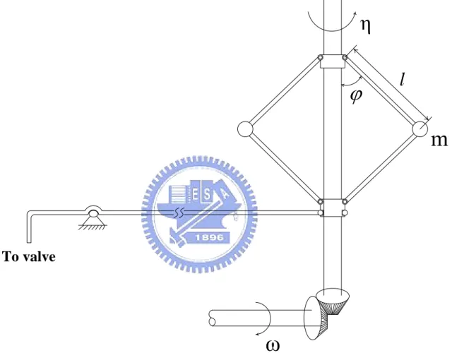
(13) Chapter 2 Regular and Chaotic Dynamics of Rotational Machine System with Centrifugal Governor. 2.1 Autonomous System The rotational machine system with centrifugal governor is shown in Fig. 2.1.1. Some basic assumptions for the system are 1. the mass of the sleeve and the rods is neglected; 2. viscous damping in the rod bearing of the fly-ball is presented by damping constant. β. From Fig. 2.1.1, the kinetic and potential energies of the system are written as follows: ⎡1 ⎤ T = 2 × ⎢ m ( l 2η 2 sin 2 ϕ + l 2ϕ& 2 ) ⎥ = ml 2η 2 sin 2 ϕ + ml 2ϕ& 2 , ⎣2 ⎦. V = −2mgl cos ϕ where l , m , ϕ and η represent the length of the rod, the mass of the fly-ball, the angle between the rotational axis and the rod, and the angular velocity of the governor, respectively. It is easy to obtain the Lagrangian. L = T − V = ml 2η 2 sin 2 ϕ + ml 2ϕ& 2 + 2mgl cos ϕ . Using the Lagrange equation, the equation of motion is derived. ϕ&& +. β m. g l. ϕ& + sin ϕ = η 2 sin ϕ cos ϕ.. (2.1.1). The net torque is the difference between the torque Q produced by the engine and the load torque QL , which is available for angular acceleration. That is,. J. dω = Q − QL dt. (2.1.2). where J is the moment of inertia of the machine. As the angle ϕ varies, the position of the control valve which admits the fuel is also varied. Their relation is presented by Refs.[37], so Eq. (2.1.2) is written in the form. 3.

(14) J ω& = γ cos ϕ − P. (2.1.3). where γ > 0 is a proportionality constant and P is an equivalent torque of the load. Usually, the governor is geared directly to the output shaft such that its speed of rotation is proportional to the engine speed, i.e. η = nω . Changing time scale τ = Ωnt , Eqs. (2.1.1) and (2.1.3) can be written in nondimensional form. ϕ&& + Cϕ& + sin ϕ = rω 2 sin ϕ cos ϕ. ω& = k cos ϕ − F. (2.1.4). where k= C=. γ. , F=. J Ωn. β mΩ n. n 2l P , r= , J Ωn g. , Ωn =. g l. and the overdot denotes differentiation with respect to τ . Eq. (2.1.4) can be expressed as three first order equations. ⎧ϕ& = ψ , ⎪ 2 ⎨ψ& = rω sin ϕ cos ϕ − sin ϕ − Cψ , ⎪ω& = k cos ϕ − F , ⎩. (2.1.5). where ψ is the angular velocity of the rod. Hence, the dynamics of the system of a rotational machine with a fly-ball governor is described by a three-dimensional autonomous system. The equilibria of the system can be found from Eq. (2.1.5) as p =[ϕ0 , 0, ω0 ] with. cos ϕ0 =. k F , ω02 = . rF k. Add slight disturbances x , y , z to the fixed point ( arccos F / k , 0,. ϕ = ϕ0 + x , ψ = y , ω = ω0 + z .. k / rF ) (2.1.6). Substitute Eq. (2.1.6) into Eq. (2.1.5), and expanding sin ϕ , cos ϕ as the Taylor series, it becomes ⎧ x& = y, ⎪ ⎨ y& = − ax − Cy + bz + HOT, ⎪ z& = − dx + HOT, ⎩. (2.1.7). where. 4.

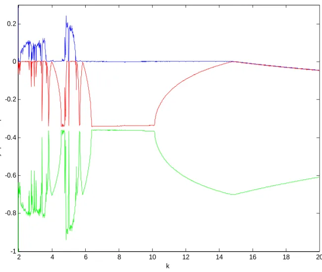
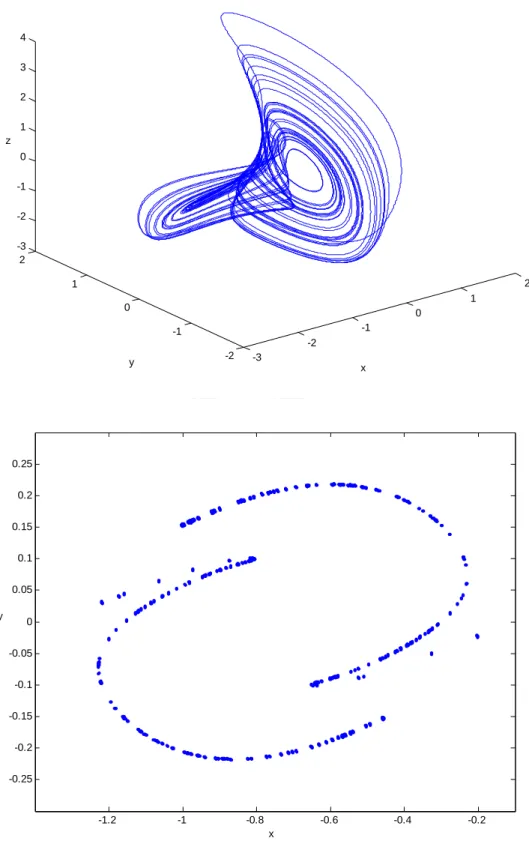
(15) a=. k2 − F2 2 rkF k 2 − F 2 , b= , d = k2 − F2 , kF k2. and the terms higher than one degree have not been written down. Let k > F > 0 , then a > 0 , b > 0 and d > 0 . By the Lyapunov instability theorem, the origin is unstable.. In order to determine the chaos existing in a nonlinear system, the method of detecting the chaos becomes very important. Here a Lyapunov exponent is used as a quantitative measure of the chaotic motion of the system. The Lyapunov exponent may be used to measure the sensitive dependence upon the initial conditions [1]. It is an index for chaotic behavior. Different solutions of the dynamical system, such as fixed point, periodic motion, quasi-periodic motion, and chaotic motion can be distinguished by it. The signs of Lyapunov exponents provide a qualitative picture of the system dynamics. Positive values of Lyapunov exponents indicate chaos, negative values of Lyapunov exponents indicate a stable orbit. In three-dimensional space, the Lyapunov exponent spectra for a strange attractor, a two-torus, a limit cycle and a fixed point are described by (＋,0,－), (0,0,－), (0, －, －) and (－,－,－), respectively.. In order to explore the chaos of the fly-ball governor system, three Lyapunov exponents are calculated when the values of parameters C , F , r are given as 0.7, 1.942, 0.25 and k is varied from 1.942 to 20. Fig. 2.1.2 illustrates the fact that some values of parameter k. will cause chaotic motion. When one defines ϕ = x , ϕ& = y , ω = z , and uses the initial conditions x(0) = 0.02 , y (0) = 0.01 , z (0) = 0.03 at: (1) k = 16 , and (2) k = 2.603 , three Lyapunov exponents are obtained, respectively,. λ1 = −0.008 , λ2 = −0.0127 , λ3 = −0.6792 , the motion of which converges to fixed point and. λ1 = 0.1116 , λ2 = 0.0 , λ3 = −0.8116 which means chaotic motion. In a dissipative system, the sum of all the Lyapunov exponents is equivalent to the negative value of the coefficient of damping in the system. Hence, the sum of the three Lyapunov exponents for the two cases (1) and (2) are －0.7. Fig. 2.1.3(a)(b) shows the phase portraits and Poincaré map of the chaotic motion at k = 2.603 .. 2.2 Nonautonomous System. 5.

(16) In the previous section, the load torque is assumed to be constant for the system. Another condition can be considered. The load torque is now not constant but is represented by a Fourier series consisting of a constant term and a series of harmonic terms. It is reasonable that the load torque of an internal combustion engine repeats after every complete working cycle. For simplicity, the form of the load torque is assumed to be F + v sin ωτ , where F , v , ω are constants. Eq. (2.1.7) is rewritten in the form. ⎧ x& = y, ⎪ ⎨ y& = − ax − Cy + bz + HOT, ⎪ z& = − dx −ν sin ωτ + HOT, ⎩. (2.2.1). where. a=. k2 − F2 2 rkF k 2 − F 2 , b= , d = k 2 − F 2 , ω = 3 and ν = 0.5 . kF k2. Lyapunov exponents are adopted for distinguishing periodic, quasi-periodic, and chaotic motions. If we choose C = 0.7 , r = 0.25 , F = 1.942 , the results is shown in Fig. 2.2.1. Poincaré map is also adopted to deal with the nonautonomous system where Poincaré section. is. prescribed. as. a. ω t = φ0 + 2nπ (φ0 = 0) plane. in. four. dimensional. space ( x, x&, z, ωt ) . Assuming that the motion of the system starts at an initial time t=t 0 , the points on the Poincaré section can be collected by a sampling of state variables at intervals of the forcing period T= 2π ω . Some numerical simulation results for different k are discussed below. The small circle in Fig. 2.2.2 for k = 17.8 indicates that the system motion is a stable harmonic motion of period 2π ω or period-1 motion. When k = 14.5 , the system motion is a quasi-periodic motion and the map will form a continuous closed orbit in the Poincaré section as shown in Fig. 2.2.3(a). If the Poincaré map appears as neither a finite set of points nor a closed orbit, the motion may be chaotic. From Fig. 2.2.3(b), chaotic motion is seen as k = 5.13 .. 6.

(17) Chapter 3 Chaos Synchronization by Linear Feedback Control and Adaptive Control. By Lyapunov stability theory and by using the coupling term, two dynamical systems will be synchronized or generalized synchronized. In the synchronized systems, one is called drive and another is called response. A lot of approaches have been proposed for the synchronization of chaotic systems which include linear and nonlinear feedback control [38-39], time-delay feedback control [40-42], adaptive control [43-45], and impulsive control [46-48]. Chaos synchronization is discussed in this chapter. Two methods are presented, the linear feedback control and the adaptive control.. 3.1 Chaos Synchronization by Linear Feedback Control Autonomous system is investigated in this section. From Eq. (2.1.7), the drive system is shown as follows: ⎧ x& = y, ⎪ ⎨ y& = − ax − Cy + bz + HOT, ⎪ z& = − dx + HOT, ⎩. (3.1.1). and the response system is shown as follows: ⎧ x& ′ = y′ + u1 , ⎪ ⎨ y& ′ = − ax′ − Cy′ + bz ′ + u2 + HOT, ⎪ z&′ = − dx′ + u + HOT, 3 ⎩. (3.1.2). where a, b, C , d are the parameters, and u1 , u2 , u3 are the controllers. Let ex = x′ − x , e y = y ′ − y , ez = z′ − z be the synchronization errors between the drive and response. systems. System (3.1.1) and (3.1.2) can be synchronized under the control:. u1 = − g x ex , u2 = 0 , u3 = − g z ez , where. α > 0 , β > 0 , gx >. (1 − a )2 , 4C. 7.

(18) gz >. 1 α β ( b 2 g x + Cd 2 − (1 − a )bd ) 2 4Cg x − (1 − a ) β α. are constants. Proof. From (3.1.1) and (3.1.2), the error dynamics can be obtained as follows:. ⎧e&x = ey − g x ex , ⎪ ⎨e&y = − aex − Cey + bez + HOT, ⎪& ⎩ez = −dex − g z ez + HOT,. (3.1.3). where ex = x′ − x , e y = y ′ − y , ez = z′ − z . Choose the following Lyapunov function:. 1 V = (α ex2 + α ey2 + β ez2 ) ≥ 0 where α , β > 0 , then the differentiation of V 2. along. trajectories of (3.1.3) is. V& = α ex e&x + α ey e&y + β ez e&z + HOT = −α g x ex2 − α Cey2 − β g z ez2 + α (1 − a)ex ey + α bey ez − β dex ez + HOT. = −eΤ Pe + HOT ,. (3.1.4). Τ. where e = ⎡⎣ ex ey ez ⎤⎦ . By Lyapunov first approximation theorem, the terms higher than second degree in the right-hand side of Eq. (3.1.4) do not influence the sign of V& and can be neglected when all the eigenvalues of coefficient matrix of the right-hand side of Eq. (3.1.4) have negative real parts. The coefficient matrix of the quadratic form in the right-hand side of Eq. (3.1.4) is. 1 1 ⎡ ⎤ − α (1 − a) βd ⎥ ⎢ α gx 2 2 ⎢ ⎥ 1 1 ⎥ ⎢ αC − αb . P = − α (1 − a) ⎢ 2 2 ⎥ ⎢ 1 ⎥ 1 ⎢ βd β gz ⎥ − αb 2 ⎣⎢ 2 ⎦⎥ To ensure that the origin of error system (3.1.3) is asymptotically stable, the matrix P should be positive definite, this is the case if and only if the following three inequalities hold: (a) α g x > 0. 1 (b) Cg x − (1 − a)2 > 0 4 1 1 1 1 (c) αβ Cg x g z + αβ bd (1 − a) − α 2b 2 g x − αβ (1 − a)2 g z − β 2Cd 2 > 0 . 4 4 4 4 8.

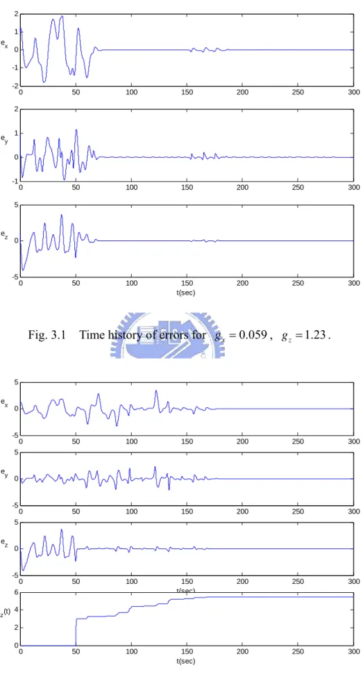
(19) Accordingly, if. (1 − a )2 gx > , 4C gz >. 1 α β ( b 2 g x + Cd 2 − (1 − a )bd ) , 2 4Cg x − (1 − a ) β α. then the matrix P is positive definite, the V& is negative definite, which implies that the origin of error system (3.1.3) is asymptotically stable. Therefore, the drive system (3.1.1) is synchronized with response system (3.1.2). In order to obtain the lower bound of g z , we need to determine the minimum function. α β. 1 α β ( b 2 g x + Cd 2 − (1 − a )bd ) , 2 4Cg x − (1 − a ) β α. f( )=. Let. α =γ , β. α β. f ( ) = f (γ ) =. 1 1 (γ b 2 g x + Cd 2 − (1 − a )bd ) , 2 γ 4Cg x − (1 − a ). f ′(γ ) =. 1 Cd 2 2 ( g xb − 2 ) , γ 4Cg x − (1 − a)2. f ′′(γ ) =. Cd 2 > 0, γ 3 4Cg x − (1 − a)2 2. f ′(γ 1 ) = 0 ,. When. γ1 =. Cd 2 . g xb2. α α Cd 2 , the function f ( ) will be at minimum. = 2 β β g xb. In numerical simulation, the parameters are a = 0.594 , b = 0.5751 , C = 0.7 , d = 1.733 . The initial condition of drive and response systems are x(0) = 0.02 , y (0) = 0.01 ,. z (0) = 0.03 , x′(0) = y′(0) = z′(0) = 1 , respectively. The lower bound of the feedback control coefficient g x =. (1 − a) 2 = 0.05887 . With this g x , the lower bound of g z = 1.228 . Now 4C. we choose g x = 0.059 and g z = 1.23 , the response system synchronizes with the drive system as show in Fig. 3.1.. 9.

(20) 3.2 Chaos Synchronization by Adaptive Control Autonomous system is investigated in this section. The drive system is shown as follows: ⎧ x& = y, ⎪ ⎨ y& = − ax − Cy + bz + HOT, ⎪ z& = − dx + HOT, ⎩. (3.2.1). and the response system is shown as follows: ⎧ x& ′ = y′ + u1 , ⎪ ⎨ y& ′ = − ax′ − Cy′ + bz ′ + u2 + HOT, ⎪ z&′ = − dx′ + u + HOT, 3 ⎩. (3.2.2). where a, b, C , d are the parameters, and u1 , u2 , u3 are the controllers. Let ex = x′ − x , e y = y ′ − y , ez = z′ − z be the synchronization errors between the drive and response. systems. System (3.2.1) and (3.2.2) can be synchronized under the control:. u1 = − g x ex , u2 = 0 , u3 = − g z ez , where g& z = θ ez2 , g z (0) = 0 , g x >. g *z >. (1 − a )2 , 4C. 1 1 (α b 2 g x + Cd 2 − (1 − a )bd ) , α > 0 , θ > 0 . 2 α 4Cg x − (1 − a ). Proof. From (3.2.1) and (3.2.2), the error dynamics can be obtained as follows:. ⎧e&x = ey − g x ex , ⎪ ⎨e&y = − aex − Cey + bez + HOT, ⎪& ⎩ez = −dex − g z ez + HOT,. (3.2.3). where ex = x′ − x , e y = y ′ − y , ez = z′ − z . Choose the following Lyapunov function:. 1 1 V = [(α ex2 + α ey2 + ez2 + ( g z − g *z )2 ] ≥ 0 where α > 0 and g *z is a constant, then the 2 θ differentiation of V along trajectories of (3.2.3) is V& = −α (ey − ex )ex − aex ey − α Cey2 + α bey ez − dex ez − g z ez2 + ( g z − g *z )ez2 = −α g x ex2 − α Cey2 − g *z ez2 + α (1 − a )ex ey + α bey ez − dex ez + HOT. = −eΤ Pe + HOT ,. (3.2.4). 10.

(21) Τ. where e = ⎡⎣ ex ey ez ⎤⎦ . By Lyapunov first approximation theorem, the terms higher than second degree in the right-hand side of Eq. (3.2.4) do not influence the sign of V& and can be neglected when all the eigenvalues of coefficient matrix of the right-hand side of Eq. (3.2.4) have negative real parts. The coefficient matrix of the quadratic form in the right-hand side of Eq. (3.2.4) is 1 1 ⎤ ⎡ − α (1 − a) d ⎢ α gx 2 2 ⎥ ⎢ ⎥ 1 1 ⎥ ⎢ αC P = − α (1 − a) − αb . ⎢ 2 2 ⎥ ⎢ ⎥ 1 1 ⎢ d g *z ⎥ − αb 2 2 ⎣⎢ ⎦⎥ To ensure that the origin of error system (3.2.3) is asymptotically stable, the matrix P should be positive definite, this is the case if and only if the following three inequalities hold: (a) α g x > 0. 1 (b) Cg x − (1 − a)2 > 0 4 1 1 1 1 (c) α Cg x g z + α bd (1 − a) − α 2b 2 g x − α (1 − a)2 g z − Cd 2 > 0 . 4 4 4 4 Accordingly, if. gx >. (1 − a ) 2 , 4C. g *z >. 1 1 (α b 2 g x + Cd 2 − (1 − a )bd ) , 2 α 4Cg x − (1 − a ). then the matrix P is positive definite, the V& is negative definite, which implies that the origin of error system (3.2.3) is asymptotically stable. Therefore, the drive system (3.2.1) is synchronization with response system (3.2.2). In numerical simulation, the parameters are a = 0.594 , b = 0.5751 , C = 0.7 , d = 1.733 . The initial condition of drive and response systems are x(0) = 0.02 ,. y (0) = 0.01 , z (0) = 0.03 , x′(0) = y′(0) = z′(0) = 1 , respectively. The lower bound of gx =. (1 − a) 2 = 0.05887 . With this g x , the lower bound of g z * = 1.228 . Now we choose 4C. g x = 0.059 , g& z = θ ez2 , θ = 1 , the response system synchronizes with the drive system as show in Fig. 3.2. 11.

(22) Chapter 4 Hyperchaos Excited by Chaos for Rotational Machine System with Centrifugal Governor. Pecora and Carroll in their pioneering paper [30] proposed a method (PC method) for synchronization by replacing the corresponding state variables of the slave system by the state variables of the master system. The difference of the method used in this chapter from PC method lies in that we replace the exciting sinusoidal function of time in nonautonomous chaotic system called excited system, by the chaotic states of variable of another chaotic system called supply system. This research is a completely new field. There appears two effects. First, hyperchaos occurs frequently and abundantly. Second, the extended chaos, i.e. anticontrol of chaos, achieves, more chaos can be obtained.. 4.1 Chaos Excited by Single Autonomous Chaos Chaotic behavior is excited by adding a chaotic signal from chaos supply system to chaos excited system. The autonomous system is chaos supply system: ⎧ x& = y, ⎪ 2 ⎨ y& = r ( z + ω0 ) sin( x + ϕ0 ) cos( x + ϕ0 ) − sin( x + ϕ0 ) − Cy , ⎪ z& = k cos( x + ϕ ) − F , 0 ⎩. (4.1.1). and the chaos excited system is: ⎧ x& ′ = y′ − v ⋅ f (t ), ⎪ 2 ⎨ y& ′ = r ( z′ + ω0 ) sin( x′ + ϕ0 ) cos( x′ + ϕ0 ) − sin( x′ + ϕ0 ) − Cy′ − v ⋅ g (t ), ⎪ z&′ = k cos( x′ + ϕ ) − F − v ⋅ h(t ), 0 ⎩ where C = 0.7 , r = 0.25 , F = 1.942 , ω = 3.0 , ν = 0.5 , cos ϕ0 =. (4.1.2). F k and ω02 = . k rF. The Lyapunov exponents are positive in the ranges 2< k <3.85, 4.66< k <5.4 for original autonomous system and in the ranges 2< k <4.12, 4.77< k <6.31 for original nonautonomous system as shown in Fig. 2.1.2 and Fig. 2.2.1 respectively. Hyperchaos is presented in following three case,. 12.

(23) (1) f (t ) ≠ 0 , g (t ) = 0 , h(t ) = 0 . The Lyapunov exponents for system (4.1.2) for which f (t ) = 0.2 x(t ) is shown in Fig. 4.1.1. Three Lyapunov exponents are (＋,+,－) which means hyperchaos, while input signal. f (t ) is chaotic for k between 2~3.85 and 4.66~5.4 and is nonchaotic for values between 3.85~4.66 and greater then 5.4 reffering to Fig. 2.1.2. That means, even f (t ) is nonchaotic, hyperchaos is presented. Besides, range of chaos is extended. When f (t ) = −0.2 x(t ) , the Lyapunov exponents is shown in Fig. 4.1.2. Chaos phenomenon is extended from 6.31(referring to Fig. 2.2.1) to 11.39. When f (t ) = 0.2 y (t ) , the Lyapunov exponents are shown in Fig. 4.1.3. Hyperchaos is presented when 4.23< k <4.84. When f (t ) = −0.2 y (t ) , the Lyapunov exponents are shown in Fig. 4.1.4. Hyperchaos is presented when 6< k <12.6. When f (t ) = −0.4 y (t ) , the Lyapunov exponents are shown in Fig. 4.1.5. Hyperchaos is presented when 10.15< k <13.3 and the chaos phenomena exist in broadest range k , 2< k <13.5, without drop-off to regular motion. When f (t ) = 0.1z (t ) , the Lyapunov exponents are shown in Fig. 4.1.6. Hyperchaos alternatively presents when 3.88< k <4.74. The chaos presents when 2< k <7.12. (2) f (t ) = 0 , g (t ) ≠ 0 , h(t ) = 0 . The Lyapunov exponents for system (4.1.2) for which g (t ) = 0.2 x(t ) is shown in Fig. 4.1.7. Chaos phenomena exist in broadest range k , 2< k <15, without decaying to regular motion. When g (t ) = −0.1x(t ) , the Lyapunov exponents are shown in Fig. 4.1.8. Hyperchaos is presented when 3.8< k <4.84. When g (t ) = −0.2 x(t ) , the Lyapunov exponents are shown in Fig. 4.1.9. Hyperchaos is presented when 4.2< k <4.84. When. g (t ) = 0.1y (t ) , the Lyapunov exponents are shown in Fig. 4.1.10. Hyperchaos is presented when 4.04< k <4.84 and 5.68< k <8.14. When g (t ) = 0.2 y (t ) , the Lyapunov exponents are shown in Fig. 4.1.11. Hyperchaos is presented when 4.22< k <4.84 and 5.95< k <8.63. When. g (t ) = 0.4 y (t ) , the Lyapunov exponents are shown in Fig. 4.1.12. Hyperchaos is presented when 4.7< k <4.84 and 6.4< k <7.5. When g (t ) = −0.05 z (t ) , the Lyapunov exponents are shown in Fig. 4.1.13. Hyperchaos is presented when 3.97< k <4.29 and 4.62< k <4.82. When. g (t ) = −0.1z (t ) , the Lyapunov exponents are shown in Fig. 4.1.14. Hyperchaos is presented when 3.92< k <4.84.. 13.

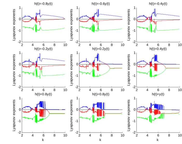
(24) (3) f (t ) = 0 , g (t ) = 0 , h(t ) ≠ 0 . The Lyapunov exponents for system (4.1.2) for which h(t ) = 0.2 x(t ) is shown in Fig. 4.1.15. Hyperchaos is presented when 5.45< k <6.4. When h(t ) = −0.8 y (t ) ~ y(t ) , the Lyapunov exponents are shown in Fig. 4.1.16. Hyperchaos is presented around 3.8~4.8 when. h(t ) = −0.8 y(t ) ~ −0.2 y (t ) ,. while. it. is. presented. around. 3.66~7. when. h(t ) = 0.2 y (t ) ~ y (t ) . When h(t ) = 0.2 z (t ) , the Lyapunov exponents are shown in Fig. 4.1.17. Hyperchaos is presented when 5.83< k <7.6. In all the above cases, extended chaos are obtained, see Table 1. From the above results, it is impressive that when the excited system is excited by a single state of autonomous chaotic system, hyperchaos occurs in most cases, while extended chaos occurs in all cases. The results are summarized in Table 1.. 14.

(25) Table 1. Hyperchaos and Extended Chaos for Excited System by Single State of Autonomous Chaotic System. Excited signal. f (t ) = 0.2 x(t ). Range of k. Range of k for. for hyperchaos. extended chaos. 5.84 ~ 6.17. 2 ~9.02. 6.47 ~ 8.49. f (t ) = −0.2 x(t ). 2 ~ 11.39. f (t ) = 0.2 y (t ). 4.23 ~ 4.84. 2 ~ 8.5. f (t ) = −0.2 y (t ). 6 ~ 12.6. 2 ~ 13.03. f (t ) = −0.4 y (t ). 10.15 ~13.3. 2 ~ 13.5. f (t ) = 0.1z (t ). 3.88 ~ 4.74. 2 ~ 7.12. g (t ) = 0.2 x(t ). 2 ~ 15. g (t ) = −0.1x(t ). 3.8 ~ 4.84. 2 ~ 6.62. g (t ) = −0.2 x(t ). 4.2 ~ 4.84. 2 ~ 6.79. g (t ) = 0.1y (t ). 4.04 ~ 4.84. 2 ~ 9.82. 5.68 ~ 8.14. g (t ) = 0.2 y (t ). 4.22 ~ 4.84. 2 ~ 9.04. 5.95 ~ 8.63. g (t ) = 0.4 y (t ). 4.7 ~ 4.84. 2~9.36. 6.4 ~ 7.5. g (t ) = −0.05 z (t ). 3.97 ~ 4.29. 2 ~ 11.9. 4.62 ~ 4.82. g (t ) = −0.1z (t ). 3.92 ~ 4.84. 2 ~ 11.94. h(t ) = 0.2 x(t ). 5.45 ~ 6.4. 2 ~11.94. h(t ) = 0.2 z (t ). 5.83 ~ 7.6. 2~ 10.08. 15.

(26) 4.2 Chaos Excited by Single Nonautonomous Chaos The nonautonomous system is chaos supply system: ⎧ x& = y, ⎪ 2 ⎨ y& = r ( z + ω0 ) sin( x + ϕ0 ) cos( x + ϕ0 ) − sin( x + ϕ0 ) − Cy, ⎪ z& = k cos( x + ϕ ) − F − v sin(ωt ), 0 ⎩. (4.2.1). and the chaos excited system is: ⎧ x& ′ = y′ − v ⋅ f (t ), ⎪ 2 ⎨ y& ′ = r ( z′ + ω0 ) sin( x′ + ϕ0 ) cos( x′ + ϕ0 ) − sin( x′ + ϕ0 ) − Cy′ − v ⋅ g (t ) , ⎪ z&′ = k cos( x′ + ϕ ) − F − v ⋅ h(t ), 0 ⎩ where C = 0.7 , r = 0.25 , F = 1.942 , ω = 3.0 , ν = 0.5 , cos ϕ0 =. (4.2.2). F k and ω02 = . k rF. The parameter ranges of chaos are extended in following three cases, (1) f (t ) ≠ 0 , g (t ) = 0 , h(t ) = 0 . The Lyapunov exponents for system (4.2.2) for which f (t ) = −0.2 x(t ) is shown in Fig. 4.2.1. The chaos is extended from 6.31(referring to Fig. 2.2.1) to 6.45. When. f (t ) = 0.4 y (t ) and -0.4 y (t ) , the Lyapunov exponents are shown in Fig. 4.2.2(a)(b). The chaos is extended to k = 10.68 and 10.86 respectively. When f (t ) = 0.1z (t ) , the Lyapunov exponents are shown in Fig. 4.2.3. The chaos is extended to k = 6.77 . (2) f (t ) = 0 , g (t ) ≠ 0 , h(t ) = 0 . The Lyapunov exponents for system (4.2.2) for which g (t ) = 0.6 y (t ) is shown in Fig. 4.2.4. The chaos is extended to 7.69. When g (t ) = −0.6 y(t ) , the Lyapunov exponents are shown in Fig. 4.2.5. The chaos is extended to k = 7.92 . (3) f (t ) = 0 , g (t ) = 0 , h(t ) ≠ 0 . The Lyapunov exponents for system (4.2.2) for which h(t ) = −0.2 x(t ) is shown in Fig. 4.2.6.. Hyperchaos. alternatively. presents. when. 2.19<. k. <4.33.. When. h(t ) = −0.8 y (t ) ~ 0.8 y (t ) , no interesting result is obtained. When h(t ) = 0.2 z (t ) , the Lyapunov exponents are shown in Fig. 4.2.7. The chaos is extended to k = 6.63 .. 16.

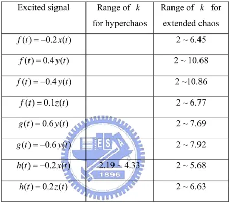
(27) From the above results, it is noted that when the excited system is excited by a single state of nonautonomous chaotic system, hyperchaos occurs in a few cases, while extended chaos occurs in most cases. The results are summarized in Table 2. Tabel 2. Hyperchaos and Extended Chaos for Excited System by Single State of Nonautonomous Chaotic System. Excited signal. Range of k. Range of k for. for hyperchaos. extended chaos. f (t ) = −0.2 x(t ). 2 ~ 6.45. f (t ) = 0.4 y (t ). 2 ~ 10.68. f (t ) = −0.4 y (t ). 2 ~10.86. f (t ) = 0.1z (t ). 2 ~ 6.77. g (t ) = 0.6 y (t ). 2 ~ 7.69. g (t ) = −0.6 y (t ). 2 ~ 7.92. h(t ) = −0.2 x(t ). 2.19 ~ 4.33. h(t ) = 0.2 z (t ). 2 ~ 5.68 2 ~ 6.63. 17.

(28) Chapter 5 Chaos, Its Control and Synchronization of Fractional Order Chaotic System. In this Chapter, the chaotic behaviors of the fractional order autonomous and nonautonomous nonlinear systems from that of rotational machine with centrifugal governor are studied. By utilizing approximation approach of fractional operator, it is found that chaos exists in the fractional order system with order less than 3. Phase portraits and bifurcation diagrams assure existence of chaotic phenomena. Observation of the bifurcation diagrams indicates behavior similar to that from the state space study in Chapter 2. By utilizing the similar scheme as that for their integral order correspondence, chaos control and chaos synchronizations are accomplished [35][49].. 5.1 Review of Fractional Operator The commonly used definition for general fractional derivative is the Riemann-Liouville definition [50]. The Riemann-Liouville definition is given here: d q f (t ) 1 dn = Γ(n − q ) dt n dt q. ∫. t. 0. f (τ ) dτ (t − τ ) q − n +1. (5.1.1). where Γ(⋅) is the gamma function and n is an integer such that n − 1 ≤ q < n . This definition is different from the usual intuitive definition of derivative. Thus, it is necessary to develop approximations to the fractional operators using the standard integral order operators. Fortunately, the Laplace transform which is basic engineering tool for analyzing linear systems is still applicable and works: q −1− k n −1 ⎧ d q f (t ) ⎫ q f (t ) ⎤ k ⎡d = − L⎨ s L f ( t ) s { } ⎬ ∑ ⎢ ⎥ , for all q , q q −1− k k =0 ⎩ dt ⎭ ⎣ dt ⎦ t =0. where n is an integer such that n − 1 ≤ q < n . Upon considering the initial conditions to be zero, this formula reduces to the more expected form. ⎧ d q f (t ) ⎫ q L⎨ ⎬ = s L { f (t )} . q ⎩ dt ⎭. (5.1.2). Linear transfer function approximations of the fractional integrator[51] is adopted. Basically 18.

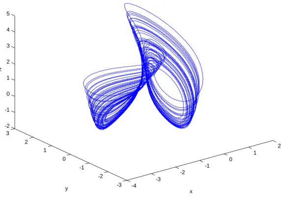
(29) the idea is to approximate the system behavior based on frequency domain arguments. [52] gives approximations for 1 s q with q = 0.1 − 0.9 in steps of 0.1. These approximations are used in the study that follows.. 5.2 The Fractional Order Autonomous Chaotic System The autonomous system is studied in this section. The standard derivative is replaced by a fractional derivative as follows: ⎧dqx ⎪ q =y ⎪ dtq ⎪d y 2 ⎨ q = r ( z + ω0 ) sin( x − ϕ0 ) cos( x − ϕ0 ) − sin( x − ϕ0 ) − Cy, ⎪ dt ⎪dqz ⎪ q = k cos( x − ϕ0 ) − F , ⎩ dt. where q is the fractional order, C = 0.7 , r = 0.25 , k = 3.5 , and ω02 =. (5.2.1). F = 1.942 , cos ϕ0 =. F k. k . Simulations are performed for q = 0.8, 0.9,1.1,1.2 . The simulation results rF. demonstrate that chaos indeed exist in the fractional order autonomous system with order less than 3. When q = 0.9 and 1.1, chaotic attractors are found and the phase portraits are shown in Fig. 5.2.1 and Fig. 5.2.2, respectively. Bifurcation diagrams which assure existence of chaotic are shown in Fig. 5.2.3 and Fig. 5.2.4. When q = 0.8 and 1.2, no chaotic behavior is found, which indicates that the lowest limit of the fractional order for this system to be chaotic may be in the range 0.8< q <0.9. Thus, the lowest order we found for this system to yield chaos is 2.7.. 5.2.1 Chaos Control Here the issue of controlling the fractional order autonomous chaotic system to its equilibrium is discussed. Simplifying the fractional order autonomous chaotic system (5.2.1) in a compact vector form, we have. dqX = f (X ) dt q. (5.2.2). with X = [ x, y, z ]T . With linear state feedback controller, Eq. (5.2.2) can be written as. dqX = f (X ) + u dt q. (5.2.3). 19.

(30) where u is a linear state feedback controller and has the following form:. u = K(X − X ) where K =diag (k1 , k2 , k3 ) , X is the control target and k1 , k2 , k3 are constant parameters. Clearly, (0, 0, 0) is always an equilibrium point of system (5.2.1). In the following simulation, we stabilize system (5.2.1) to this equilibrium point. Standard stability analysis easily shows that with (k1 , k2 , k3 ) = (−1, 0, −1) , the equilibrium (0, 0, 0) of the controlled integral order chaotic system is locally stable and is shown in Fig. 5.2.5. Simulation results show that this controller can also stabilize the fractional order chaotic system to this equilibrium. The trajectories of the controlled fractional order chaotic system with q = 0.9 and q = 1.1 are shown in Fig. 5.2.6 and Fig. 5.2.7, respectively. The control signal is added at t = 500s and 200s respectively. The designed chaos controller can effectively and fast control the fractional order chaotic systems to its equilibrium point X = (0, 0, 0) .. 5.2.2 Chaos Synchronization of the Same Fractional Order systems Here the issue of chaos synchronization of system (5.2.1) is discussed. Consider the drive-response synchronization scheme of autonomous chaotic systems. dqX = f (X ) dt q. (5.2.4). dqX′ = f ( X ′) + u dt q. (5.2.5). where q is the fractional order. u is a linear state feedback controller and has the following form:. u = K(X ′ − X ) where K = diag (k1 , k2 , k3 ) , k1 , k2 , k3 are constant parameters. Define the error state as e = X ′ − X , synchronization can be achieved when e(t ) → 0 as t → ∞ .. Next, we numerically study the synchronization in two cases. Case 1. q = 0.9 , K = diag (−1, 0, −1) . Controller is added at t = 300 s , and response system is synchronized at t = 341s as shown in Fig. 5.2.8.. 20.

(31) Case 2. q = 1.1 , K = diag (−1, 0, −1) . Controller is added at t = 300 s , and response system is synchronized at t = 315s as shown in Fig. 5.2.9.. 5.2.3 Chaos Synchronization of Different Fractional Order systems Here the issue of chaos synchronization of different order systems is discussed. Consider the drive-response synchronization scheme of autonomous chaotic systems. dqX = f (X ) dt q. (5.2.6). d pX′ = f ( X ′) + u dt p. (5.2.7). where q and p are different. u is a linear state feedback controller. As the method utilized in last section, synchronization can be practically achieved. Next, we numerically study the synchronization in two cases. Case 1. q = 0.9 , p = 1.1 , K = diag (−1000, −1000, −1000) . Controller is added at t = 200 s , and response system is practically synchronized as shown in Fig. 5.2.10. Case 2. q = 1.1 , p = 0.9 , K = diag (−1000, −1000, −1000) . Controller is added at t = 200 s , and response system is practically synchronized as shown in Fig. 5.2.11.. 5.3 The Fractional Order Nonautonomous Chaotic System The nonautonomous system is studied in this section. The standard derivative is replaced by a fractional derivative as follows: ⎧dqx ⎪ q = y, ⎪ dtq ⎪d y 2 ⎨ q = r ( z + ω0 ) sin( x − ϕ0 ) cos( x − ϕ0 ) − sin( x − ϕ0 ) − Cy, ⎪ dt ⎪dqz ⎪ q = k cos( x − ϕ0 ) − F −ν sin ω t , ⎩ dt. 21. (5.3.1).

(32) where q is the fractional order, C = 0.7 , r = 0.25 , k = 2.8 ,. ω = 3 , cos ϕ0 =. F = 1.942 , ν = 0.5 ,. F k and ω02 = . Simulations are performed for q = 0.8, 0.9,1.1,1.2 . The k rF. simulation results demonstrate that chaos indeed exist in the fractional order nonautonomous system with order less than 3. When q = 0.9 and 1.1 , chaotic attractors are found and the phase portraits are shown in Fig. 5.3.1 and Fig. 5.3.2, respectively. Bifurcation diagrams which assure existence of chaotic are shown in Fig. 5.3.3 and Fig. 5.3.4. When q = 0.8 and 1.2 , no chaotic behavior is found, which indicates that the lowest limit of the fractional order for this system to be chaotic is q = 0.8 − 0.9 . Thus, the lowest order we found for this system to yield chaos is 2.7.. 5.3.1 Chaos Control Here the issue of controlling the fractional order nonautonomous chaotic system to periodic motion is discussed. Simplifying the fractional order nonautonomous chaotic system (5.3.1) in a compact vector form, we have. dqX = f ( X ) + g (t ) dt q. (5.3.2). with X = [ x, y, z ]T . With linear state feedback controller, Eq. (5.3.2) can be written as. dqX = f ( X ) + g (t ) + u dt q. (5.3.3). where u is a linear state feedback controller and has the following form: u = KX. where K = diag (k1 , k2 , k3 ) , k1 , k2 , k3 are constant parameters. In the following simulation, we control system (5.3.1) to period motion. With (k1 , k2 , k3 ) = (−1, 0, −1) , the integral order chaotic system can be controlled to periodic motion and is shown in Fig. 5.3.5. Simulation results show that this controller can also control the fractional order chaotic system to periodic motion. The trajectories of the controlled fractional order chaotic system with. q = 0.9 and q = 1.1 are shown in Fig. 5.3.6 and Fig. 5.3.7, respectively. The control signal is added at t = 40 s . The designed chaos controller can effectively and fast control the fractional order chaotic system to periodic motion.. 22.

(33) 5.3.2 Chaos Synchronization of the Same Dractional Order Systems Here the issue of chaos synchronization of system (5.3.1) is discussed. Synchronization is achieved by linear feedback method. Consider the drive-response synchronization scheme of two nonautonomous chaotic systems. dqX = f ( X ) + g (t ) dt q. (5.3.4). dqX′ = f ( X ′) + g (t ) + u dt q. (5.3.5). where q is the fractional order. u is a linear state feedback controller and has the following form:. u = K(X ′ − X ) where K = diag (k1 , k2 , k3 ) , k1 , k2 , k3 are constant parameters. Define the error state as e = X ′ − X , synchronization can be achieved when e(t ) → 0 as t → ∞ .. Next, we numerically study the synchronization in two cases. Case 1. q = 0.9 , K = diag (−1, 0, −1) . Controller is added at t = 300 s .and response system is synchronized at t = 310 s as shown in Fig. 5.3.8. Case 2. q = 1.1 , K = diag (−1, 0, −1) . Controller is added at t = 300 s .and response system is synchronized at t = 320 s as shown in Fig. 5.3.9.. 5.3.3 Chaos Synchronization of Different Fractional Order Systems Here the issue of chaos synchronization of different order systems is discussed. Consider the drive-response synchronization scheme of autonomous chaotic systems. dqX = f ( X ) + g (t ) dt q. (5.3.6). d pX′ = f ( X ′) + g (t ) + u dt p. (5.3.7). where q and p are different. u is a linear state feedback controller. As the method. 23.

(34) utilized in last section, synchronization can be practically achieved. Next, we numerically study the synchronization in two cases. Case 1. q = 0.9 , p = 1.1 , K = diag (−1000, −1000, −1000) . Controller is added at t = 300 s , and response system is synchronized as shown in Fig. 5.3.10. Case 2. q = 1.1 , p = 0.9 , K = diag (−1000, −1000, −1000) . Controller is added at t = 300 s , and response system is synchronized as shown in Fig. 5.3.11.. 24.

(35) Chapter 6 Conclusions. A lot of researches have shown that chaotic phenomena are observed in many physical systems that possess nonlinearity. For the nonlinear system, the study of the types of system behavior, the effects to the behavior caused by different signal, the behavior analysis of the system, consist of the major tasks. In this thesis, integral and fractional order rotational machine system with centrifugal governor are investigated. By applying various numerical results, such as time history analysis, phase portraits, bifurcation diagrams, the behavior of the chaotic motion are presented. In Chapter 2, the governing equations of motion are formulated, Lyapunov exponents are used to detect the chaos existing in the system. In Chapter 3, linear feedback control method and adaptive control method for chaos synchronization are proposed by using Lyapunov first approximation theorem and asymptotical stability theorem. Numerical simulation is provided to show the effectiveness of our method. By using Lyapunov first approximation theorem, we can achieve the synchronization of more complex system such as rotational machine system in this thesis. In Chapter 4, we devotes to a new concept of hyperchaos and extended chaos driven by states of chaotic system instead of driven by sinusoidal functions of time. Many interesting results are obtained. If chaos is driven by the state of autonomous system, hyperchaos are presented frequently. And the ranges of chaos are extended. If chaos is driven by the state of nonautonomous system, its performance is less fruitful as that driven by the state of autonomous system. Fractional calculus is a 300-yerar-old mathematical topic. Although it has a long history, the applications of fractional calculus to physics and engineering are just a recent focus of interest. In Chapter 5, we study the chaotic behaviors in the fractional order autonomous and nonautonomous nonlinear systems of rotational machine system with centrifugal governor. It is shown that systems with total order less than three exhibit chaos as well as its integeral order system. Phase portraits and bifurcation diagrams assure existence of chaotic phenomena. By utilizing the similar scheme as that for their integral order correspondence, chaos control and chaos synchronization are accomplished, in which chaos synchronizations of different fractional order systems need large coupling strength to be synchronized. 25.

(36) η. ϕ. l. m. To valve. ω. Fig. 2.1.1 Physical model of a rotational machine with a fly-ball governor system.. 26.

(37) 0.2. Lyapunov exponents. 0. -0.2. -0.4. -0.6. -0.8. -1. 2. 4. 6. 8. 10. 12. 14. 16. k. Fig. 2.1.2 Three Lyapunov exponents for k between 1.942 and 20.. 27. 18. 20.

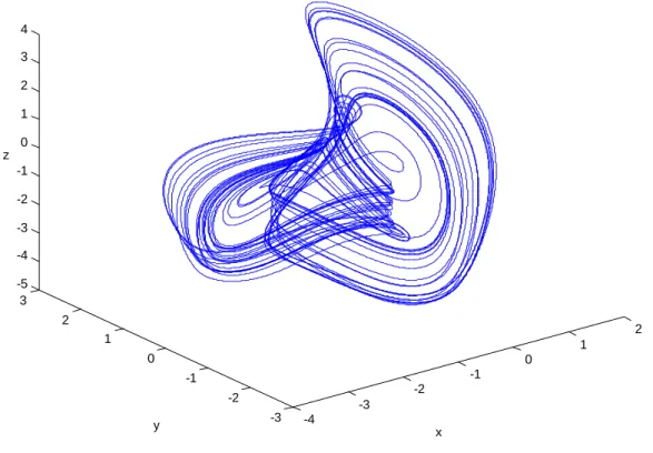
(38) 4 3 2 1 z 0 -1 -2 -3 2 2. 1 1. 0. 0 -1. -1 -2 -2. y. -3 x. 0.25 0.2 0.15 0.1 0.05 y. 0 -0.05 -0.1 -0.15 -0.2 -0.25. -1.2. -1. -0.8. -0.6. -0.4. -0.2. x. Fig. 2.1.3 (a) Phase portrait (b) Poincaré map for k = 2.603 .. 28.

(39) 0.4. 0.2. Lyapunov exponents. 0. -0.2. -0.4. -0.6. -0.8. -1. 2. 4. 6. 8. 10. 12. 14. 16. k. Fig. 2.2.1 Three Lyapunov exponents for k between 1.942 and 20.. 29. 18. 20.

(40) (a). 1.5. 1. 0.5 z 0. -0.5. -1 0.6 0.4. 0.15 0.1. 0.2. 0.05 0. 0. -0.05 -0.2. -0.1 -0.4. y. -0.15 -0.2 x. (b). 1.5. 1 (0.13331,0.18034,0.64699) 0.5 z 0. -0.5. 0.2. -1 0.6. 0.1 0.4. 0. 0.2 0 -0.2. -0.1 -0.4. -0.2 x. y. Fig. 2.2.2 (a) Phase portrait (b) Poincaré map for k = 17.8 .. 30.

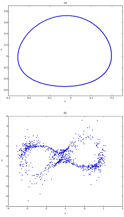
(41) (a) 0.8. 0.6. 0.4. 0.2 y 0. -0.2. -0.4. -0.6 -0.3. -0.2. -0.1. 0. 0.1. 0.2. x. (b) 4. 3. 2. 1. 0 y -1. -2. -3. -4. -5 -4. -3. -2. -1. 0. 1. x. Fig. 2.2.3 Projection of Poincaré map of: (a) quasi-periodic (b) chaotic motion on x − y plane.. 31. 2.

(42) 2 1 ex. 0 -1 -2. 0. 50. 100. 150. 200. 250. 300. 0. 50. 100. 150. 200. 250. 300. 0. 50. 100. 150 t(sec). 200. 250. 300. 2. ey. 1 0 -1 5. ez. 0. -5. Fig. 3.1 Time history of errors for g x = 0.059 , g z = 1.23 .. 5 ex. 0. -5. 0. 50. 100. 150. 200. 250. 300. 0. 50. 100. 150. 200. 250. 300. 0. 50. 100. 150 t(sec). 200. 250. 300. 0. 50. 100. 150 t(sec). 200. 250. 300. 5 ey. 0. -5 5 ez. 0. -5 6 gz (t) 4 2 0. Fig. 3.2 Time history of errors for g x = 0.059 , θ = 1 . 32.

(43) 1. Lyapunov exponents. 0.5. 0. -0.5. -1. -1.5. 2. 3. 4. 5. 6 k. 7. 8. 9. 10. Fig. 4.1.1 Three Lyapunov exponents for k between 2 and 10, f (t ) = 0.2 x .. 1 0.8 0.6. Lyapunov exponents. 0.4 0.2 0 -0.2 -0.4 -0.6 -0.8 -1. 2. 4. 6. 8. 10. 12. 14. k. Fig. 4.1.2 Three Lyapunov exponents for k between 2 and 15, f (t ) = −0.2 x .. 33.

(44) 1. Lyapunov exponents. 0.5. 0. -0.5. -1. 2. 3. 4. 5. 6 k. 7. 8. 9. 10. Fig. 4.1.3 Three Lyapunov exponents for k between 2 and 10, f (t ) = 0.2 y .. 1. Lyapunov exponents. 0.5. 0. -0.5. -1. -1.5. 2. 4. 6. 8. 10. 12. 14. k. Fig. 4.1.4 Three Lyapunov exponents for k between 2 and 15, f (t ) = −0.2 y .. 34.

(45) 1.5. 1. Lyapunov exponents. 0.5. 0. -0.5. -1. -1.5. 2. 4. 6. 8. 10. 12. 14. k. Fig. 4.1.5 Three Lyapunov exponents for k between 2 and 15, f (t ) = −0.4 y .. 35.

(46) (a). 1. Lyapunov exponents. 0.5. 0. -0.5. -1. 2. 3. 4. 5. 6 k. 7. 8. 9. 10. Fig. 4.1.6 (a) Three Lyapunov exponents for k between 2 and 10, f (t ) = 0.1z .. (b). 0.25. Lyapunov exponents. 0.2. 0.15. 0.1. 0.05. 0. -0.05. 2. 2.5. 3. 3.5. 4. 4.5. 5. 5.5. 6. 6.5. k. Fig. 4.1.6. (b) Locally enlarged figure for (a).. 36. 7. 7.5.

(47) 1. Lyapunov exponents. 0.5. 0. -0.5. -1. 2. 4. 6. 8. 10. 12. 14. k. Fig. 4.1.7 Three Lyapunov exponents for k between 2 and 15, g (t ) = 0.2 x .. 1. Lyapunov exponents. 0.5. 0. -0.5. -1. -1.5. 2. 3. 4. 5. 6 k. 7. 8. 9. 10. Fig. 4.1.8 Three Lyapunov exponents for k between 2 and 10, g (t ) = −0.1x .. 37.

(48) 1 0.8 0.6. Lyapunov exponents. 0.4 0.2 0 -0.2 -0.4 -0.6 -0.8 -1. 2. 3. 4. 5 k. 6. 7. 8. Fig. 4.1.9 Three Lyapunov exponents for k between 2 and 8, g (t ) = −0.2 x .. 0.8. 0.6. 0.4. Lyapunov exponents. 0.2. 0. -0.2. -0.4. -0.6. -0.8. -1. -1.2. 2. 3. 4. 5. 6 k. 7. 8. 9. 10. Fig. 4.1.10 Three Lyapunov exponents for k between 2 and 10, g (t ) = 0.1y .. 38.

(49) 1. Lyapunov exponents. 0.5. 0. -0.5. -1. 2. 3. 4. 5. `. 6 k. 7. 8. 9. 10. Fig. 4.1.11 Three Lyapunov exponents for k between 2 and 10, g (t ) = 0.2 y .. 1. Lyapunov exponents. 0.5. 0. -0.5. -1. -1.5. 2. 3. 4. 5. 6 k. 7. 8. 9. 10. Fig. 4.1.12. Three Lyapunov exponents for k between 2 and 10, g (t ) = 0.4 y .. 39.

(50) 1. Lyapunov exponents. 0.5. 0. -0.5. -1. -1.5. 2. 3. 4. 5. 6. 7 k. 8. 9. 10. 11. 12. Fig. 4.1.13 Three Lyapunov exponents for k between 2 and 12, g (t ) = −0.05 z .. 1. Lyapunov exponents. 0.5. 0. -0.5. -1. -1.5. 2. 3. 4. 5. 6. 7 k. 8. 9. 10. 11. 12. Fig. 4.1.14 Three Lyapunov exponents for k between 2 and 12, g (t ) = −0.1z .. 40.

(51) 1 0.8. 0.6. Lyapunov exponents. 0.4. 0.2 0. -0.2. -0.4. -0.6 -0.8. -1 2. 3. 4. 5. 6. 7 k. 8. 9. 10. 11. Fig. 4.1.15 Three Lyapunov exponents for k between 2 and 12, h(t ) = 0.2 x .. 41. 12.

(52) h(t)=-0.6y(t). 2. 4. 6 8 h(t)=-0.2y(t). 10 Lyapunov exponents. 1 0 -1 -2. 2. 4. 6 8 h(t)=0.8y(t). 10. 1 0 -1 -2. 2. 4. 6 k. 8. 10. Lyapunov exponents. -2. 0 -1 -2. 2. 4. 6 8 h(t)=0.2y(t). 10. 1. Lyapunov exponents. -1. h(t)=-0.4y(t). 1. 0 -1 -2. 2. 4. 6 8 h(t)=0.8y(t). 10. 1. Lyapunov exponents. Lyapunov exponents. 0. Lyapunov exponents. Lyapunov exponents. Lyapunov exponents. Lyapunov exponents. h(t)=-0.8y(t) 1. 0 -1 -2. 2. 4. 6 k. 8. 10. 1 0 -1 -2. 2. 4. 6 8 h(t)=0.4y(t). 10. 2. 4. 6 h(t)=y(t). 8. 10. 2. 4. 6 k. 8. 10. 1 0 -1 -2 1 0 -1 -2. Fig. 4.1.16 Three Lyapunov exponents for k between 2 and 10, h(t ) = −0.8 y (t ) ~ 1y (t ) .. 42.

(53) 1. Lyapunov exponents. 0.5. 0. -0.5. -1. -1.5. 2. 3. 4. 5. 6. 7 k. 8. 9. 10. 11. Fig. 4.1.17 Three Lyapunov exponents for k between 2 and 12, h(t ) = 0.2 z .. 43. 12.

(54) 0.2. 0.1. 0. Lyapunov exponents. -0.1. -0.2. -0.3. -0.4. -0.5. -0.6. -0.7. -0.8. 2. 3. 4. 5. 6 k. 7. 8. 9. Fig. 4.2.1 Three Lyapunov exponents for k between 2 and 10, f (t ) = −0.2 x .. 44. 10.

(55) 0.2. 0.1. 0. Lyapunov exponents. -0.1. -0.2. -0.3. -0.4. -0.5. -0.6. -0.7. -0.8. 2. 4. 6. 8. 10. 12. 14. k. Fig. 4.2.2 (a) Three Lyapunov exponents for k between 2 and 15, f (t ) = 0.4 y .. 0.2. 0. Lyapunov exponents. -0.2. -0.4. -0.6. -0.8. -1. 2. 4. 6. 8. 10. 12. 14. k. Fig. 4.2.2 (b) Three Lyapunov exponents for k between 2 and 15, f (t ) = −0.4 y . 45.

(56) 0.4. 0.2. Lyapunov exponents. 0. -0.2. -0.4. -0.6. -0.8. -1. 2. 3. 4. 5 k. 6. 7. Fig. 4.2.3 Three Lyapunov exponents for k between 2 and 8, f (t ) = 0.1z .. 46. 8.

(57) 0.2. 0.1. 0. Lyapunov exponents. -0.1. -0.2. -0.3. -0.4. -0.5. -0.6. -0.7. -0.8. 2. 3. 4. 5. 6 k. 7. 8. 9. Fig. 4.2.4 Three Lyapunov exponents for k between 2 and 10 g (t ) = 0.6 y .. 47. 10.

(58) 0.2. 0.1. 0. Lyapunov exponents. -0.1. -0.2. -0.3. -0.4. -0.5. -0.6. -0.7. -0.8. 2. 3. 4. 5. 6 k. 7. 8. 9. Fig. 4.2.5 Three Lyapunov exponents for k between 2 and 10 g (t ) = −0.6 y .. 48. 10.

(59) 0.4. 0.2. Lyapunov exponents. 0. -0.2. -0.4. -0.6. -0.8. -1. 2. 2.5. 3. 3.5. 4. 4.5. 5. 5.5. 6. 6.5. k. Fig. 4.2.6 (a) Three Lyapunov exponents for k between 2 and 6.5 h(t ) = −0.2 x .. 0.15. Lyapunov exponents. 0.1. 0.05. 0. -0.05. -0.1. 2. 2.5. 3. 3.5. 4. k. Fig. 4.2.6 (b) Locally enlarged figure for (a). 49. 4.5.

(60) 0.2. Lyapunov exponents. 0. -0.2. -0.4. -0.6. -0.8. 2. 3. 4. 5 k. 6. 7. Fig. 4.2.7 (a) Three Lyapunov exponents for k between 2 and 8 h(t ) = 0.2 z .. 50. 8.

(61) 5 4 3 2 z 1 0 -1 -2 3 2. 2. 1. 1 0. 0 -1. -1. -2. -2 y. -3 -3. -4 x. Fig. 5.2.1 Phase portrait of the fractional order autonomous system with order q = 0.9.. 51.

(62) 4 3 2 1 0 z -1 -2 -3 -4 -5 3 2. 2. 1. 1 0. 0 -1. -1. -2. -2 y. -3 -3. -4 x. Fig. 5.2.2 Phase portrait of the fractional order autonomous system with order q = 1.1.. 52.

(63) Fig. 5.2.3 Bifurcation diagram of the fractional order autonomous system with order q = 0.9.. 53.

(64) Fig. 5.2.4 Bifurcation diagram of the fractional order autonomous system with order q = 1.1.. 54.

(65) 2 0 x -2 -4. 0. 50. 100. 150. 200 t. 250. 300. 350. 400. 0. 50. 100. 150. 200 t. 250. 300. 350. 400. 0. 50. 100. 150. 200 t. 250. 300. 350. 400. 4 2 y. 0 -2 -4 4 2. z. 0 -2 -4. Fig. 5.2.5 Time history of the state variables of the controlled integral order autonomous system with order q = 1.. 55.

(66) 2 0 x -2 -4. 0. 100. 200. 300. 400 t. 500. 600. 700. 800. 0. 100. 200. 300. 400 t. 500. 600. 700. 800. 0. 100. 200. 300. 400 t. 500. 600. 700. 800. 4 2 y. 0 -2 -4 6 4. z. 2 0 -2. Fig. 5.2.6 Time history of the state variables of the controlled fractional order autonomous system with order q = 0.9.. 56.

(67) 2 0 x -2 -4. 0. 50. 100. 150. 200 t. 250. 300. 350. 400. 0. 50. 100. 150. 200 t. 250. 300. 350. 400. 0. 50. 100. 150. 200 t. 250. 300. 350. 400. 4 2 y 0 -2 5. z. 0. -5. Fig. 5.2.7 Time history of the state variables of the controlled fractional order autonomous system with order q = 1.1.. 57.

(68) 4 2 ex. 0 -2 -4. 0. 50. 100. 150. 200. 250 t. 300. 350. 400. 450. 500. 0. 50. 100. 150. 200. 250 t. 300. 350. 400. 450. 500. 0. 50. 100. 150. 200. 250 t. 300. 350. 400. 450. 500. 4 2 ey. 0 -2 -4 10. ez. 5 0 -5. Fig. 5.2.8 Time history of errors of the fractional order autonomous system with order q = 0.9.. 58.

(69) 5. ex. 0. -5. 0. 50. 100. 150. 200. 250 t. 300. 350. 400. 450. 500. 0. 50. 100. 150. 200. 250 t. 300. 350. 400. 450. 500. 0. 50. 100. 150. 200. 250 t. 300. 350. 400. 450. 500. 4 2 ey. 0 -2 -4 10 5. ez. 0 -5 -10. Fig. 5.2.9 Time history of errors of the fractional order autonomous system with order q = 1.1.. 59.

(70) 2. ex. 0 -2 -4. 0. 50. 100. 150. 200. 250 t. 300. 350. 400. 450. 500. 0. 50. 100. 150. 200. 250 t. 300. 350. 400. 450. 500. 0. 50. 100. 150. 200. 250 t. 300. 350. 400. 450. 500. 4 2 ey. 0 -2 -4 5. ez. 0. -5. Fig. 5.2.10 Time history of errors of different fractional order autonomous systems with order q = 0.9 and p = 1.1.. 60.

(71) 4. ex. 2 0 -2. 0. 50. 100. 150. 200. 250 t. 300. 350. 400. 450. 500. 0. 50. 100. 150. 200. 250 t. 300. 350. 400. 450. 500. 0. 50. 100. 150. 200. 250 t. 300. 350. 400. 450. 500. 4 2 ey. 0 -2 -4 5. ez. 0. -5. Fig. 5.2.11 Time history of errors of different fractional order autonomous systems with order q = 1.1 and p = 0.9.. 61.

(72) 2. 3 2. 1. 1 y. z. 0. 0 -1. -1. -2 -3. -2. -1 x. 0. -2 -3. 1. -2. -1 x. 0. 1. -1. 0 y. 1. 2. 3 4. 2. 2. 1. z. z 0. 0. -2 2 0 y. -1. 2 0 -2. -4. -2 x. -2 -2. Fig. 5.3.1 Phase portrait of the fractional order nonautonomous system with order q = 0.9.. 62.

(73) 2. 4. 1. 2. 0. 0. y. z -1. -2. -2. -4. -3 -4. -2. 0. -6 -4. 2. -2. 0. x. 2. x. 4 5. 2. 0. 0. z. z -5. -2. -10 5 2. 0 y. -4. 0 -5. -4. -2 x. -6 -3. -2. -1. 0. 1. 2. y. Fig. 5.3.2 Phase portrait of the fractional order nonautonomous system with order q = 1.1.. 63.

(74) Fig. 5.3.3 Bifurcation diagram of the fractional order nonautonomous system with order q = 0.9.. 64.

(75) Fig. 5.3.4 Bifurcation diagram of the fractional order nonautonomous system with order q = 1.1.. 65.

(76) 1 0 x. -1 -2 -3. 0. 50. 100. 150 t. 200. 250. 300. 0. 50. 100. 150 t. 200. 250. 300. 0. 50. 100. 150 t. 200. 250. 300. 2 1 y 0 -1 2 0 z -2 -4. 0.2. 0.1. z. 0. -0.1. -0.2 0.04 0.03 0.02. 0.015. 0.01. 0.01. 0. 0.005 -0.01. 0 -0.02. -0.005 -0.03. y. -0.01 -0.04. -0.015. x. Fig. 5.3.5 Time history of the state variables of the controlled integral order nonautonomous system with order q = 1.. 66.

(77) 1 0 x. -1 -2 -3. 0. 50. 100. 150 t. 200. 250. 300. 0. 50. 100. 150 t. 200. 250. 300. 0. 50. 100. 150 t. 200. 250. 300. 1 0.5 y. 0 -0.5 -1 2 1 z. 0 -1 -2. 0.2. 0.1. z. 0. -0.1. -0.2 0.04 0.02. 0.015 0.01. 0. 0.005 0. -0.02. -0.005 -0.01. y. -0.04. -0.015. x. Fig. 5.3.6 Time history of the state variables of the controlled fractional order nonautonomous system with order q = 0.9.. 67.

(78) 2 0 x -2 -4. 0. 50. 100. 150 t. 200. 250. 300. 0. 50. 100. 150 t. 200. 250. 300. 0. 50. 100. 150 t. 200. 250. 300. 2 1 y. 0 -1 -2 4 2. z. 0 -2 -4. 0.15 0.1 0.05 0 z -0.05 -0.1 -0.15 -0.2 0.03 0.02. 0.01. 0.01 0.005. 0 0. -0.01 -0.005. -0.02 y. -0.03. -0.01 x. Fig. 5.3.7 Time history of the state variables of the controlled fractional order nonautonomous system with order q = 1.1.. 68.

(79) 0.2 0.1 ex. 0 -0.1 -0.2. 0. 50. 100. 150. 200. 250 t. 300. 350. 400. 450. 500. 0. 50. 100. 150. 200. 250 t. 300. 350. 400. 450. 500. 0. 50. 100. 150. 200. 250 t. 300. 350. 400. 450. 500. 0.2 0.1 ey. 0 -0.1 -0.2 0.4 0.2. ez. 0 -0.2 -0.4. Fig. 5.3.8 Time history of errors of the fractional order nonautonomous system with order q = 0.9.. 69.

(80) 4 2 ex. 0 -2 -4. 0. 50. 100. 150. 200. 250 t. 300. 350. 400. 450. 500. 0. 50. 100. 150. 200. 250 t. 300. 350. 400. 450. 500. 0. 50. 100. 150. 200. 250 t. 300. 350. 400. 450. 500. 2. ey. 0 -2 -4 5. ez. 0. -5. Fig. 5.3.9 Time history of errors of the fractional order nonautonomous system with order q = 1.1.. 70.

(81) 4 2 ex. 0 -2 -4. 0. 50. 100. 150 t. 200. 250. 300. 0. 50. 100. 150 t. 200. 250. 300. 0. 50. 100. 150 t. 200. 250. 300. 2 1 ey. 0 -1 -2 5. ez. 0 -5 -10. Fig. 5.3.10 Time history of errors of different fractional order nonautonomous systems with order q = 0.9 and p = 1.1.. 71.

(82) 4 2 ex. 0 -2 -4. 0. 50. 100. 150 t. 200. 250. 300. 0. 50. 100. 150 t. 200. 250. 300. 0. 50. 100. 150 t. 200. 250. 300. 2 1 ey. 0 -1 -2 10. ez. 5 0 -5. Fig. 5.3.11 Time history of errors of different fractional order nonautonomous systems with order q = 1.1 and p = 0.9.. 72.

(83) REFERENCES [1] G. Chen, X. Dong, From Chaos to Order, World Scientific, New Jersey, 1998. [2] A. Pikovsky, M. Rosenblum, and J. Kurths, Synchronization: A Universal Concept in Nonlinear Science, Cambridge Univ. Press, Cambridge, 2001.. [3] G.V. Osipov, B. Hu, C. Zhou, M.V. Ivanchenko, and J. Kurths, “Three types of transitions to phase synchronization in coupled chaotic oscillators”, Phys. Rev. Lett., Vol. 91, 024101, 2003. [4] S. Chen, D. Wnag, L. Chen, Q. Zhang, C. Wang, “Synchronizing strict-feedback chaotic system via a scalar driving signal”, Chaos, Vol. 14, pp. 539-544, 2004. [5] G. Millerioux, J. Daafouz, “Input independent chaos synchronization of switched systems”, IEEE Trans. Automat. Contr., Vol. 49, pp. 1182-1186, 2004. [6] S. Tang and J.M. Liu, “Chaos synchronization in semiconductor lasers with optoelectronic feedback”, IEEE J. Quantum Electron., vol. 39, pp. 708-715, 2003. [7] Y. Wang, Z.H. Guan, and H.O. Wang, “Feedback and adaptive control for the synchronization of chen system via a single variable”, Phys. Lett. A, Vol. 312, pp. 34-40, 2003. [8] M. Feki, “Observation-based exact synchronization of ideal and mismatched chaotic systems”, Phys. Lett. A, Vol. 309, pp. 53-60, 2003. [9] S. Bowong and F.M.M. Kakmeni, “Synchronization of uncertain chaotic systems via backsteeping approach”, Chaos, Solitons & Fractals, Vol. 21, pp. 999-1011, 2004. [10] H.K. Khailil, Nonlinear Systems, Prentice Hall, New Jersey, 2002. [11] J.M.T. Thompson and H.B. Stewart, Nonlinear Dynamics and Chaos, Wiley, New York, 2002. [12] J.C. Sprott, Chaos and Time-Series Analysis, Oxford University Press, New York, 2003. [13] G. Chen, Controlling chaos and bifurcation in engineering systems, CRC Press, Boca Raton, 2000. [14] T. Wu, M.S. Chen, “Chaos control of modified Chua’s circuit system”, Physica D, Vol. 164, pp. 53-58, 2002. [15] E.V. Bondarenko and I. Yevin, “Music and control of chaos in the brain”, Physics and Control, Proceedings. 2003 International Conference , Vol. 2, pp. 497-500, 2003. [16] H. Korn and P. Faure, “Is there chaos in the brain? II. Experimental evidence and related models”, C. R.Biologies, Vol. 326, pp. 787-840, 2003. 73.

(84) [17] M.W. Lee, Y. Hong, and K.A. Shore, “Experimental demonstration of VCSEL-based chaotic optical communications”, IEEE Photonics Technology Lett., Vol. 16, no. 10, pp. 2392-2394, 2004. [18] J. Paul, S. Sivaprakasam, and K.A. Shore, “Dual-channel chaotic optical communications using external-cavity semiconductor lasers”, J. Opt. Soc. Amer. B, Vol. 21, pp. 514-521, 2004. [19] J. Garcia-Ojavo and R. Roy, “Parallel communication with optical spatiotemporal chaos”, IEEE Trans. Circuits Syst. I, Vol. 48, pp. 1491-1497, 2001. [20] P. Davis, Y. Liu, and T. Aida, “Versatile signal generation in chaotic optical communication devices modeled by delay-differential equations”, Nonlinear Analysis, Vol. 47, pp. 5729-5739, 2001. [21] I. Radojicic, D. Mandic, and D. Vulic, “On the presence of deterministic chaos in HRV signals”, Computers in Cardiology 2001 , pp. 465-468. [22] V.K. Yeragan and R. Rao, “Effect of nortriptyline and paroxetine on measures of chaos of heart rate time series in patients with panic disorder”, J. Psychosom. Res., Vol. 55, pp. 507-513, 2003. [23] K.M. Cuomo and V. Oppenheim, “Circuit implementation of synchronized chaos with application to communication”, Phys. Rev. Lett., Vol. 71, pp. 65-68, 1993. [24] L. Kocarev and U.Parlitz, “General approach for chaotic synchronization with application to communication”, Phys. Rev. Lett., Vol. 74, pp. 5028-5031, 1995. [25] J. Lu, X. Wu, amd J. Lü, “Synchronization of a unified chaotic system and the application in secure communication”, Phys. Lett. A 305, pp. 365-370, 2002. [26] J. Amirazodi, , E.E. Yaz, , A. Azemi, , Y.I. Yaz, “Nonlinear observer performance in chaotic synchronization with application to secure communication”, Proceedings of the 2002 IEEE International Conference on Control Applications, IEEE. Part Vol.1, pp.76-81, 2002. [27] G. Hu, Z. Feng, and R. Meng, “Chosen ciphertext attack on chaos communication based on chaotic synchronization”, IEEE Trans. Circuits Syst. I, Vol. 50, pp. 275-279, 2003. [28] S. Celikovsky, G. Chen, “Secure synchronization of a class of chaotic systems from a nonlinear observer approach”, IEEE Trans. Automat. Contr., Vol. 50, pp. 76-82, 2005. [29] H.K. Khalil, Nonlinear Systems, Third edition, Prentice Hall, New Jersey, 2002. [30] L.M. Pecora and T.L. Carrol, “Synchronization in chaotic systems”, Phys. Rev. Lett. Vol. 64, pp. 821-824, 1990. 74.