On weak residual error estimation

ON

WEAK

RESIDUAL

ERROR

ESTIMATION*

JINN-LIANG LIU

Abstract, A generalframework for weak residualerrorestimators applyingtovarioustypesofboundaryvalue problemsinconnectionwithfiniteelementandfinitevolumeapproximationsisdeveloped. Basic ideascommonly sharedbyvarious applications in error

estimation

and adaptive computationarepresentedand illustrated. Some

numericalresultsaregiventoshowthe effectiveness and efficiency of the estimators.

Keywords,adaptivity,aposteriorierrorestimates,finiteelement,finitevolume,variationalproblems

AMS subjectclassifications.65N30,65N50,35J20, 35J60

1. Introduction. Adaptivity is a trend incontemporarycomputationalscience. The re-markableadvances inadaptive methodologyfor finite elementapplicationssince thepioneer

workby Babuka and Rheinboldt [7] have had aprofound impact on practical, large-scale computations.

There are fourtypes ofadaptivitywhich can be identifiedby the letters r

(relocating

nodes),h

(mesh

sizehrefinement),p(spectralorder pincrement),andhp (both hrefinement and pincrement). Alladaptivemethodsrequiremoreor less aposterioriinformation aboutthe

computedsolutionforoptimizingoverallcomputationalefforts in the sense that the methods deliver agivenlevel ofaccuracywitha minimum ofdegreesof freedom.

In

essence, thea posteriorierror estimation canberegardedasthe heart of the adaptivemechanism. Inthe

developmentof a posteriori error estimators, three main approaches maybe distinguished [22], [29], namely,those based on residual,postprocessing,orinterpolationtechniques. Our

estimatorsherefollow the firstapproach.

In

the firstapproach ithas becomepracticallystandardtospecifythe interior residuals intermsof thegoverningdifferentialequationandtomeasuretheboundaryresidualsbythe

jumps in the normal derivatives on the interfaces between elements; see [3], [4], [6], [7], [8], 11], 19]. The various error estimators then differessentiallyin theway thejumps are handled.

In

contrast, we considerhere error equations (or inequalities)in which the right side isaresidual of thecomputedsolution inweak form. It appears tobe naturaltocall the

resultingerror estimatesweak residual estimators.

A

specialcase,ofthe estimators seemsto be firstproposed by AdjeridandFlahertyin 1]. The weak residualerrorestimators tendto be morewidely applicablesince, in many applications, the governingequation maynotbe available in differentialform.

In

recentyears, there has beengrowingevidence, intheory as

wellasin application, showingthepromiseof the use of weak residual estimators; see[1], [2], [9], [21], [25].

Thispaper attemptstogive an overall view of the weak residual error estimation in con-nection with theadaptiveprocess,different numericalmethods,and varioustypesofboundary

valueproblems. The numericalschemes ofparticularinterestbelongto twofamilies ofwidely

usedmethodsnthe finite element method

(FEM)

and the finite volume method

(FVM).

All estimatorspresentedhere canbeextractedto twobasic components whichareweak residuals andcomplementary

_finite

element(FE)spaces. Twotypes ofcomplementary spacescanbe classified. One istheconforming typewhichtogetherwiththeoriginal

FE

space preserves

thecontinuity across adjacent

FEs.

This in turncorresponds to an elementwise error esti-mation using error residuals onlyinteriorto elements. The estimators used in [1], [2], [9],

*ReceivedbytheeditorsMay24, 1993;acceptedfor publication(inrevisedform)April 24, 1995. Thiswork

wassupportedinpart by NSC grant82-0208-M-009-060, Taiwan,ROC.

tDepartment

of Applied Mathematics, National Chiao Tung University, Hsinchu, Taiwan (jinnliu@math. nctu.edu.tw).

1249

[25] areof this type. The otheristhe nonconforming typewhichinstead uses both interior andboundaryresiduals foreach element. Itis shown in[21 that thenonconformingtype is

independentof the

FE

order used for thecomputedsolution, whereas the conforming type

considers more

closely

theeffect of the order of the

FEs

1],[8]. While thisstudyisnot

com-prehensive,wedo illustrate thetwocomponentsin error estimation and theadaptive process byfour modelproblems; namely,weconsiderellipticboundaryvalueproblems, parametrized

nonlinear equations, symmetrichyperbolicequations, andvariationalinequalities.

In

2,

the error estimators are derived inageneralframeworkbymeansof abstract varia-tional formulations. Definitions, notation, and basic ideas are then introducedalongthe course of the derivation. Althoughthe estimators arenotrestrictedtoany particular typeofadaptivity,

wealso discussbrieflyastandard h-refinementstrategyintwospacedimensions. In

3,

the four modelproblemsand thetwonumericalmethodsarespecificallyusedtodemonstrate how

theycan becastintothegeneralframework. Finally,in

4,

numerical results aregivenwith

respecttoeach subsection in

₃

toshow the effectivenessandefficiencyof the estimators.

2. Backgroundand basic ideas. The aim of thispaperistooffer,totheextentpossible,

aglobalviewof the use ofweak residual error estimators. Itisinstructivetosummarize some fundamental features which constitute variousadaptivemethods for various modelproblems

considered herein.

2.1. Abstract variationalproblems.

Let

f2 be a boundedregion in the plane with a

Lipschitz boundaryOf2

Of2z

U 0"2Nand

H

k(f2)andH (1-’), I" C 0, be theusualSobolev

spaces equippedwith the norms

_II"

_Ilk

and].

Ir,

r, respectively.

Let

H(f2) C

Lz(f2)

be a Sobolev space equippedwith the norm

]1.

]].

For simplicity, we assumethat all functions in

H()

satisfy a homogeneous Dirichletboundary condition on O f2z, ifany.

Let

K

be a closed convex subset ofH(f2). Let F

H()

--+ R be a continuous linear form. Let B(., .)

H(S2)

x

H(S2)

--+ Rbe a bilinear form such that there existtwopositiveconstants

/3,

6and anonnegativeconstantofor which

(2.1)

(2.2)

B(u,v) <

fl]]ul]

]]vll, u,v E H(f2), (u,u) >_

allull

2-

llullg,

u e

We

shall consideraclass ofvery general problemsinan abstract variationalsetting: Find u E Ksuch that

(2.3)

B(u,

v)

F(v)

> B(u,u)

F(u)

’v

K.

Dependingonthe definition of the closed convexset

K

and thepropertiesof the bilinear form

B,

the abstract variationalproblem

(2.3)

cangive various equivalentformulations of

problems which willbe exemplifiedin

_3.

Discussions ofwell-posedness of the problem

(2.3),

in some selectivesettings,canbefound, e.g.,in[13], [18].

2.2.

FE

spaces. To discretize

(2.3),

we introduce S a finite-dimensional subspace of

H

()

characterizedbyamesh sizeh and associated with aregular,butnotnecessarily quasi-uniform,triangulation

7-

onS2. To approximate

K,

weconstruct aclosed convex subset

_Ks

ofS. Theapproximateproblemof

(2.3)

isthentofindUs 6

Ks

such that

(2.4) B(us,

Our objectiveistopresent various error formulationsonwhich various aposteriorierror estimatorsassessingtheexacterrorbetween the solutionsuand

_us

of

(2.3)

and(2.4), respec-tively,arebased. All estimators can be extractedto twobasic components--weakresiduals andcomplementary

FE

spaces. Wefirstdiscussthecomplementary spaces.

For

the sake ofefficiency,the estimatorswillbebasedonlocalcomputations. Weintroduce somelocal functionspacesthat we willrequire. Associated with

T,

letSbe anotherlarger

FE

subspace ofH(f2), i.e., S C

.

Let

H(r) denote the restriction of

H()

to r 6

7-and

HT-(S2)

_l-IeT-

H(r)

denote thespace ofpiecewise

H(f2)

functions.

For

instance, if

H (S2)

H

(f2),then

_HT-

(f2)willbe thespace ofpiecewise H functions.

For

v,win

HT-

(f2),

wedefinethe brokenL2_{innerproductand normby (v, w)}

YeT-(v,

w),

Ilvll

(v, v),

analogously,

the brokenH(f2) norm,

Ilvl[

2

_Yv7

Ilvll(.

Note

thatH(f2) C HT-(f2) C

L2()

and the above definitions reducetothe usual ones whenever v, ware inH(f2).

Let

be split intotwosubspaces

S

S

,

SC)S

{0}. Let

_S

denote therestrictionofS to r 6

T

and let

Sr

1--It,7-

s.

We

shall consider inparticularthe splitting

(2.5)

7-

S

S,

Sfq

S-

_{0},

Sr

_{7 0.}

Thespaces

_S

and $7- arespacesof piecewise polynomialslocallydefined ineach element r in

7-.

Note

the inclusions C

7

C HT-(f2) and S C

Sr.

The error estimatorsgiven

in

₃

willbe calculated in thecomplementary space

_S-.

We assumethat the bilinear form

Bcan define an innerproduct B(.,

.)

on

7

and with it theenergynorm

_Iwl

2 B(w,

w).

Allerrorestimatorsbelow aremeasured in this norm,although,intheory, theyarenotstrictly

restrictedtothisnorm.

2.3. Abstract variational error formulation. Lete u Usdenote theexact errorof the approximate solution

us.

Wenow derive ageneralformulationfor theexacterror interms of theapproximatesolution. Substitutingu e

+

_us

intoproblem (2.3),wehave

B(e,v) F(v)

+

B(us, v)

> B(e,e)

+

B(e,

us)

+

B(us,

e)

+

B(us,

Us)

F(e) F(us)

Vv

K.

Note

that the bilinear form

B

can be nonsymmetric.

By

rearranging terms in the above

inequality,we can rewrite this as

B(e,v Us) [F(v

> B(e,e)

[F(e)

B(us,e)] Vv6 K.

The left-hand side of theinequalityclearly suggests thatwe can definethe following new closed convex subsetby translating the original convexsetK with respecttothecomputed

solution us"

K’--

K-Us C H(f2).

Moreover,

byvirtueof the boundedness of the bilinear formB and the linear functionalFon

H (f2),the Rieszrepresentationtheorem shows that there exists auniquelinearfunctional

G

on

H

(f2) definedby

(2.6)

G(w)

F(w) B(us,w)

’w

H(S2).

We

callGaweak residual in contrasttothe usual formulation in which the residual is interms of thegoverningdifferential equation usedby manyauthors [8], [11], [19].

The error estimation is then based on the following new variational (error) problem:

Determine e 6 K such that

(2.7) B(e,w) G(w) > B(e,

e)

G(e)

The reason we use the weak residual formG instead of the governing equationistwofold. First, since

_us

is itself anapproximatesolution, its second derivative, for second-orderpartial

5 8 4 13

0 7 16 18 11 2

FIG. 2.1. 1-irregular meshrefinement.

differentialequations (PDEs), in thesense of distribution willfurther incur error. Second,

formany applications, thegoverning differential equation may not be available, i.e., only

theintegralform is available. Forsuch cases, the formulation of errorproblemslike

(2.7)

is certainly moregeneral.

2.4.

A

mesh refinement

strategy.

There aremany refinement strategies proposedin the literature. The error estimatorspresentedhere arenotrestrictedtoanyparticularadaptive

refinement.

In

fact,it has been shown in[21 that there isnoorder restrictionfor the

FE

spaces

used in theapproximatesolutionorin the error estimation; thatis, theerrorestimators canbe used in connection withanyone of theh-, p-, orhp-versions of the

FEM. In

the numerical

experiments,to test ourerrorestimators(see

4),

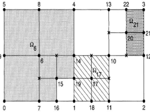
weuse inparticularthe so-called 1-irregular mesh refinementstrategyfirstproposedin[7] and later detailed in 14]. Sincethe refinement scheme hasbeen extendedtoincludeadaptivefinitevolumecomputations,webriefly discuss its basicfeatures.

Recall thatanode is calledregularifit constitutesa vertexfor each of theneighboring

elements; otherwise it is irregular.

Figure

2.1 shows a particular 1-irregularmeshwhere irregular nodes markedby areallof index-1 irregularity,that is, the maximum number of

irregularnodesonanelement side is one.

In

implementation,nodegreesof freedom will be associatedwiththeseirregularnodes.

Hence,

supportsof theshapefunctionsdefiningabasis for an

FE

spacechange adaptivelywith mesh refinements; forexample,theshaded subdomains

f26, f217,and

f2el

arethesupportsoftheshapefunctionscorresponding, respectively,tothe

regularnodes6, 17,and 21 inFig.2.1. The

FE

spacessoconstructedpreservethe conformality

required bythe standard

FE

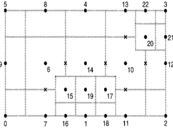
approximation provided that some special element constraint methods are usedtoinvokecontinuityacross interelement boundariesofelements of different sizeand withshapefunctionsofdiffering polynomialdegree [14].

For finite volume approximation, control volumes have to adapt accordingly to their dual elements. Let/ denote the dual mesh for7-.

Note

that theFVM requires a control volume foreachregularnode wheredegreesoffreedom are defined. Thus,inparticular,23 control volumesin the dual mesh of Fig. 2.1 are constructed andshown, bydotted lines, in

Fig. 2.2. Notice that thepatternof the boundaries of control volumes appearinginelements

maydifferelementbyelement. Thisplaysan essential role in theimplementationsincemost

computations, approximations,aswellaserror estimations, aretobeperformedelementwise before the assemblingprocess.

3. Modelproblemsand numerical methods.

We

nowapply

the

generalformulations and the basic ideas discussed above to four modelproblems in connection with

FEM

and

FVM.

5 8 4 13 22 3 0 o .21 20i

9.

o i o i o

:

_.12 6 14 10 o o o 15 19 17: +, I, 0 7 16 18 11 2

FIG.2.2. Adaptive control volumes.

Sincethe aposteriorierror estimation isthe heart of acomplete selfadaptivemechanism, we stressparticularlyvarious errorequationsorinequalitieson which the errorestimatorsare based. Some rigoroustheories ofthe estimators can be found in [2], [21 ].

We

first note that if theclosed convex set Kin

(2.3)

isitself the Sobolev space H(f2),

then theinequality

(2.3)

reducestoa variational equation. In

3.1-3.3,

3.5 wewilladdress thisequalityform.

3.1. Elliptic boundaryvalueproblems. Considertheboundaryvalueproblem

Lu

:--

-V.

(aCx)VuCx))

₊

bCx)uCx)

_f

Cx) in

(3.1) _Ou

u--0 on

O’D,

_{a(X)-’--g(x)}

on

O"N.

The associated variationalproblemis tofindu

H(2)

such that

(3.2)

BCu,

v)

(f,

v)

₊

(g,

V)Oau

’V’V

H(f2),

where

H(fl)

{u

e

HI()

u 0onOD}, B(u, v) "=

f

(aVuVv

+

buy)dx,

(f

v)"=

fa

_f

vdx, {g,

V}aau

"=

f

gv ds. "U

To

beginwithandtoavoid technical details, wealways assumetheuniquesolvability of the variationalproblemsconsidered here and below.

Note

thatwedonot assumethe coefficient functionb(x)in

(3.1)

tobestrictly positiveinS2, hence the error estimatorstobegiven apply

toindefiniteproblemsaswell[21 ].

Correspondingto

(2.4)

and(2.7),theapproximationand errorproblemsfor

(3.2)

areto determineUs 6 Sande 6 H (f2) such that

(3.3)

B(Us,V)

Cf, v)

+

(g,

v}OaN

’V’V

e S

and

(3.4)

BCe,

v)

-BCus, v)

₊

(f, v)

+

(g,

V}Oau

YV

HCf2),

respectively,wherethecomputed

FE

solutionUs canonlybe assessedaposteriori, i.e., after itsavailability.

Since thespace H() is still infinite dimensional and the discretization of(3.4)inthe

original

FE

space S only producestrivial estimated errors,

(3.4)

has to be solved in alarger space S.

However,

thiswould cause the error calculationtobeimpractically expensive since

(3.4)will result in a larger

system

ofequationsthan that of

(3.3). Hence,

the use of the

complementary subspaces appears tobe natural. Nevertheless, if thesubspaceis chosento be S

c,

the error calculationmay involve aglobalsolutionto asystemof equations.

We

are thereforeledtoconsider thecomplementary subspaces

_S-

C HT-(S’2) and, consequently,to solve thefollowingreducedproblem: Determine 6

_S(ri),

ineach element"gi

IT,

such that

(3.5)

B(g,

v)

-B(u,,

v)

₊

(f,

v)

₊

(g,

V)Oau

YV

_Sr(ri).

Note

that if

_S-

C

H

(),aconformingsubspace, theunique solvabilityof

(3.5)

can be ensured as that of

(3.3)

andonlythe interior residual in each element will be used. Onthe otherhand,if

_S-

C

HT-(S2)

but not in

H

(2),anonconformingsubspace,then

(3.5)

results in anonconforming solution scheme [13] and the estimation willinclude both interior and

boundaryresidualsforeach element. With some moderate assumptions on the bilinear form and thecomplementary spaces(sufficientlylarge),itis shownin

[21

that theuniquesolvability for suchproblemsstillholds.

As noted already, the error residuals can be expressed in either differential or weak form.

We

brieflydescribe thedifferences between thesetwoapproaches. Formoredetailed theoreticalinvestigationwereferthereaderto 11],[21 ].

Let

Ebe the collection ofcurves which forms anedgeof an element r in T.Thesetof

edges maybedecomposedasthe unionoftwodisjointsetsE

_EB

U

EI,

where

_EB

istheset ofedgesonOand

E1

isthesetofedgesin the interior of

.

Foreachedgeein

E,

we define anormal directionn

_ne.

More

specifically,

n

istheusual outward normal when e 6

E

while, for e6

EI,

its choice isarbitrary.

Let

tin,’out be two elementssharinganedgeein

_Ez

andsupposethat the normalnisoutward fromtin. Then, for xone, thejump and theaverage

of v onearedefined,respectively,by

1

[V]J(X)

)(X)]out-

)(X)ll-in

and [VJA(X

_{)(X)l-gou

+

)(X)lz’in

},

Substituteu e

+

_us

into

(3.1)

andmultiply bya test functionv;then we obtain, in each element r,

(3.6)

(Le, v)r -(Lus,

v)r

₊

(f,

v)r,

where

_Lus

is definedin the

sense

of distributions. Now integration by partsofthe lefttermin

(3.6)

yields

(3.7)

(ge,

v)r

B(e, v)

a-n,

v

+

a--n

v

Er Er

andaftersumming

(3.6)

overall elements, we find that

(3.8)

B(e, v)

(f

Lus,

v)

₊

g

-a-n

V

+

a--n

v

ON J E1

This isthe standard formulation forestimatingerrorsusedby manyauthors[7],[8], 11], 19]. Onthe otherhand,if theterm(Lus,

v)

in

(3.6)

isrewritten as in(3.7),then in each element

r, we obtain

B(e,v)r _{a_-SS} v -B(u,v)r

₊

(f,

v)r.

Hence

a summationoverall elementsleadsto

B e,v a

-n

V F

,

a

-n

j

[V]A)

-B(us,v)

₊

(f,

v), E1

whichgives

(3.4)

with more generaltest functions v E HT-(f2) if theexact solutionu isin

H2(2).

It

isnecessarytoreusethe differentialoperator Lwhen the estimators arecalculated based on

(3.8). In

contrast, intermsof

(3.4),

the same bilinear formulation

(3.2)

canbe used in both

approximationand error estimation. This is certainlypreferable,from the

user’s

viewpoint, in

adaptive implementation.

Moreover,

theformalapproachcanonlyutilizethecomplementary spaces

_S-

in anonconforming settingwhilethe weak residualapproach maybeused in either aconformingoranonconformingsetting. Finally,in 11],thefollowingsaturation condition isintroducedfor thespaces used in the erroranalysis:

(3.9)

Ilu

ulll

+

_h/2

[

a

Ou-ul

I

_<

p(h)211u

_ull2,

On _J

where

.

u

istheapproximatedsolution(for analytical purposes only) soughtinthelarger spaces

It

isassumed that

_limh-0

p 0; that is, hashigherorder than S. Onthe otherhand, in weak form, the saturation condition is asfollows:

Ilu-ullpllu-u,ll, 05p<l.

Thus the condition

(3.10)

is somewhat weaker than

(3.9)

sinceitallows the

FE

ordersofS

and tobeequal (see, e.g., [21] andExample4.2

below).

The introduction of thejumpsin thenormal derivative of thecomputedsolutionsatinterelement boundariesactuallyforces p tobecomelargerand hence deteriorates the quality of the error estimator[21]. Almost all

differential-typeresidual error estimators[3], [4], [7], [8], 11], 19] requiresomecompatibility

conditionsorauxiliarylocalproblemstoovercome this intrinsicdifficulty simplybecausethe distributionandjumptermsare included inthe residual, i.e., theright-handsideof

(3.8).

These conditions orproblemsaresomewhat ad hoc dependingstronglyonthe modelproblemunder consideration; see the above references. Thecomplementary spaces are essential for both differentialand weak residualapproaches. Withthe weak residualform, one canconcentrate

primarilyonthe construction of theshapefunctionsof

_Sr,

which can stillhandlejumpsacross element boundaries(withanonconforming setting),iftheyare dominant errors.

The norm

_II1111;

--: Oi, for eachelementz’i E

’,

is called theerror indicatorofthe

element which assesses thequalityof theapproximatesolution

us

inthiselement and indicates whether theelement needstobe refined, derefined, orunchanged. Summingoverallelements,

theerror estimatorforUscanbe definedby

II1111

Y]i

Theerrorestimator canserve as one ofthemajor stoppingcriteria for an entireadaptive process.

Thequalityof aproposederror estimator isusuallytestedbyvarious modelproblemstowhich

theexactsolutions areexplicitlyknown.

A

computableeffectivity index 0=

isusuallyintroducedtoquantifythequalityof the estimatorand,consequently,thequalityof theapproximatesolution.

3.2. Parametrized nonlinearequations. Stationary problemsformany scientific and

engineeringproblemsaremodeledbyaparameter-dependent equation

(3.11)

F(u,)) =0,

where u is a state variable, 2 is a d-dimensional parameter vector, and F denotes some differentialoperatoronasuitablestate space. Typically,the solution set

M

F

-1

₍₀₎

turns outtobe a differentiable submanifold

M

of dimension d of theproduct

X

of the statespace

andtheparameter space. This can beensured, for instance, when

F

is aFredholmmapof indexd onX [23].

Allstandard discretizations of aparametrized boundaryvalueproblem

(3.11)

leave the parametervectoruntouched and henceapproximatetheequationsbysomefinite-dimensional system Fs(us,

)

0.

Hence,

under suitable conditions, we may expect the solution set

Ms

F-I

(0)

to be ad-dimensional submanifold of some discretizationspace

Xs.

Frequently,

Xs

canbe embedded in X and then the discretization errorrepresentssome measure of the distancebetween

M

and

_Ms

inX.

Our

goalnow is to estimatethe discretization error. There aretwomajorissuesfor the error estimationof

_Ms.

The first issueisefficiency.

It

isintrinsicallymoreexpensivefor nonlinear

parametrizedproblemsthan it is for linearproblems. Thesecond issue isconsistency.

It

is wellknown [23]that the parameterdependencecausesthe discretization errortobecome a local concept whichdependsonthe choice of the local coordinatesystemon themanifold.

For

instance, in the continuationmethod,wemustoften fix a local coordinatesystemforcalculating

severalpointsonthe manifold and thenchangethe coordinatesystemasneeded, and so on.

However,

for error estimation, the coordinate system isusually fixed, [23], throughoutthe entiremanifoldand hence isnotapplicablenearany foldpointwithrespecttotheparameter space. Themainwaytoresolve these difficulties istouse linearizationand a local coordinate

system.

At

anyx0 (u0,)0) 6

M,

we define alocal coordinatesystemthat satisfiesthefollowing

conditions:

(3.12)

X=WT,

dimT=d,

WkerDF(xo)={O}.

it isshown in[25]that the constrained linearized(infinite-dimensional) problem

(3.13)

F

(Xs)

₊

D F (Xs)CO O, rc

(CO)

O,

for

(3.11)

has auniquesolutionco _{x0 Xs} 6 Wwhichistheexact errorofthe approximate solution

xs

(Us,)s).

Here

7r 6

L(X)

is anaturalprojectionof

X

onto

T

along

W.

The

FE

approximation of

(3.11)

isofinteresthere.

We

consider, inparticular, thefollowingmildly nonlinearproblem: Find(u, .) 6

H

(f2) x

A

such that

(3.14)

(F(u,)), v) :=

j

[a(k,

)Vu Vv

+

g(u,),

)v]

d

0

Yv

6

H0(fl),

where

F

X

H

(S2) x

A

--+

Y

H

-1

_(f2)

_{and the coefficient functionsa and g aregiven}

sothat theproblemiswellposed.

Apparently, the nonlinearproblem

(3.14)

does not fit into the general variational for-mulationgivenin theprevious section.

However,

itsweak residual form can becastinthe framework of the variational errorsetting.

In

weak form

(3.13)

requiresthe deterrnination of

(w,/x)

E

Hd

x Asuchthat

(3.5)

(3.16)

B(w,v)

₊

C(#,v) -(F(us, ‘ks),

v)

Yv e

H

(f2), rr(w,

t)

=0, where B(w, v)

:=

_Ja(.a(‘ks,

)Vw

Vv

₊

gu(us,‘ks,

)wv) d,

c(..

.) .= _.)v.,

v,

+

_(gz(Us,,ks,

)

#)v)

d.

At

any computedpoint (us, ‘ks) e

Ms,

our aposteriorierrorestimates thusrequirethe determinationof

(t,/2)

6

_Sr(ri)

x A such that

(3.17)

B(t,

v)

₊

C@,

v) -(F(us, ‘ks),

v) Yv

S("ci)

(3. 8)

zr(,

)

=0.

The choiceof the local coordinate systematany pointx0on.Misarbitraryaslongas it

satisfiesthe conditions in

(3.12). By

definition, the local coordinate system

(3.12)

and hence the constraint

7r(co,/x)

0 canchange frompointto pointonthe solution manifold.

We

choose T

kerDF(xo)

inparticular. The constraint

(3.18)

is then equivalentto

(t,/2)

6

Ws

Xs

C) Wwhichis orthogonalto the d-dimensionalsubspace

T

kerDFs(xs) of

Xs

correspondingtothetangent spaceof

_Ms

atthecomputed pointXs. If

A

is one dimensional and astandard continuationprocessisused, then a normalizedtangentvector isusuallyavailable ateachcomputed point. Analogously,inthemultiparametercase, if atriangulationof

Ms

is

computed bythe method of[24],thenagainorthonormal bases of thetangent spaceareavailable at the computed points onthe manifold. This uniform treatment of the aposteriori error estimation alongthecomputedmanifold

Ms

avoids aforementioned

difficulties. Moreover,

the introductionof the linear,local,solutionscheme ensures that the method iscomputationally relatively inexpensive.

An

aposteriorierror estimation has beendevelopedforstronglynonlinearequationswith ascalarparameterin[27]. There theasymptoticexactnessof a residual estimator wasproved

under suitablehypotheses. Tsuchiya’s approach requiresone to fix the local coordinatesystem

intwostages.

In

the firststagebefore the turning point, the system is definedbythenatural

parameter.

In

the secondstagewhen the continuationprocess is nearand after theturning point,thesystemisthenrotatedby90degreesthusallowingamoreelaborate error estimate neartheturning point.

In

the senseof the definition of the local coordinatesystem,this is a

specialcase of ourapproach.

Moreover,

Tsuchiya’sapproach requiresaglobalsolutiontothe linearizedresidualequationsfor error estimation.

3.3. Symmetric hyperbolic equations.

In

thetheory of

PDEs

thereis afundamental distinctionbetween those ofelliptic, hyperbolic,andparabolic types. Thetheoryofsymmetric positivedifferentialequations developed byFriedrichs 17]isknown for its unified treatment,

analytically aswell asnumerically,for

PDEs

thatchangetype within the domain of interest such as the Tricomi problem and forward-backward heat equations.

In

the development

of the error estimator for the Friedrichs system, we use inparticularthe

FEM proposed

by

Lesaint[20].

An

unknown p-dimensional vector-valued function defined on f2 is given by u

(ul,_u2

Up)

r.

Let

f

(fl,

f2

fp)

Tbeagiven p-dimensional vector-valued function

definedonf2. Lettheoperators

L

and

M

be definedbyand consider the followingsystems: 2

Ou

(3.19)

Lu(x)

:--

E

_Ai(x)-ff--

₊

Ao(x)II

f(x)

for x

i=1

(3.20)

Mu(x)

:= (#(x)

(x))u(x)

0 forx

where/3

Y=I

niAi, the

ni’s

beingthecomponentsof theouternormalon0f2. Thematrices

Ai, 1,2,aresymmetric, Lipschitzcontinuousinx (xl, x2)for x

f.

The coefficients of the matrix

_A0

(x)

ofL (RP) arebounded in f2. The

matrix/z (x)

of

L

(Rp) is defined for x

a

sothat theboundarycondition

(3.20)

is admissibleand theoperator

L

is positive in the sense of Friedrichs 17];i.e.,

(i) #(x)

+/z*

(x)

ispositive semidefinite on0f2, (ii) Ker(/z

-/3)

@Ker(/z

,+/3)

R

p_{on0f2, and} (iii)

A0

+

a

_-’=l

oai _{>_Co1 Yx6,}

where/z*

and

_A

areadjointmatrices

of/z

andA0, respectively,

co

isapositiveconstant,and

Iisthe identity matrix.

Theadjoint operators L*andM*of

L

and

M

are defined,respectively, by

(3.21)

(3.22)

2 0

_,

L*v(x)

"=

-/.=

xi

(Ai(x)v(x))at-

Ao(x)v(x)

Vx

M*v(x)

:=

(/z*(x)

+/3(x))v(x) ’v’x

6

Let

(q, g) :=

_fa

q(x). g(x)dx and(q, g) "=

f0a

q"gds,whereq.g

₌₁

qigi.One variational formulationof(3.19)and

(3.20)

istofindu 6

(H

(f2))p such that

1

(3.23)

B(u,

v)

_(Lu,

v)

₊

_(u,

L’v)

+

_(/zu,

v)

(f,

v)

Vv

6

(HI())

p.

For

any given approximatesolutionu, 6

(S)

p C

(H

(f2))p of(3.23),againanalogousto

(2.7),the error estimator

(3.23)

canthen be calculatedby solvingthe reduced errorproblem:

Determine 6

(S-)

psuch that

(3.24) B(fi, v)

(f,

v) B(u,

v)

Vv

_(Sr)

p.

Since the boundary conditions

(3.20)

and

(3.22)

for test and trial functions u and v, respectively, are different, this would make itimpossible toshow thecoercivityin asimple

manner iftheadjoint operator L*werenotincluded in

(3.23).

Withthe formulation of

(3.23)

and Friedrichs’s identities 17],thecoercivityisguaranteedin[20]butonlyinthe lower-order norm, i.e.,

II0, instead

of thegeneral Grding-type inequality (2.2).

3.4. Variationalinequalities.

In

theprevioussubsections, in terms of abstractsettings,

theclosed convexset

K

isthe SobolevH

(S2)

itself. This inturnleads to variationalequations

for theprecedingmodelproblems.

In

this subsection, we deal with variational inequalities

formulated in thegeneral form(2.3)where now the

K

is indeedaclosed convex subset of

H (). As

we would inatypicalproblem,weshall now also consider the abstract

minimization

problem: Findu 6 Ksuchthat

(3.25)

J (u) inf J (v),

vEK

ONWEAK RESIDUAL ERROR ESTIMATION 1259

where the functional J H(f2) --+ R is definedby

1

J(v)

-

(v, v) F(v),

providedthat the bilinear formB(., .)is symmetric andH(f2)-elliptic,i.e.,ot 0 in

(2.2).

Correspondingto

(2.4),

(3.25)

reducestothe finite-dimensionalapproximate problem

(3.26)

J(us) inf J(vs),

Vs Ks

which, under suitable conditions on the approximate convexset

K

[16], [18]canbe solved

bymathematicalprogramming subjecttoa finitenumber of constraints inducedby

Ks.

Clearly, the variational error problem (2.7) suggeststhe needed formulation for error

estimation;that is, determine

Y

6 K such that

(3.27)

B(,

w)-

G(w)

>

B(, )- G(,)

Vw

_K.,

where

_K

is acomplementary closed convexsetof

_Sr

under similar conditions as those of

Ks.

Inequality

(2.7)

alsosuggeststhat a new functional can be defined intermsof theweak residualG, namely,

1

E(W)

-

B(w, w) a(w).

Consequently,wehavethefollowingreduced minimizationproblem: Determine 6 K such that

(3.28)

E(g) inf E(w).

weKc

3.K The finite vlume element method. There aremanyvariantsof

FVMs. We

con-siderspecificallythe finitevolume element method

(FVEM). As

noted in[12], the FVEM

was developedas anattempttouse

FE

ideas tocreate amoresystematicfinitevolume

(FV)

methodology. The basicideais toapproximatethe discrete fluxes needed inFV by replacing

the unknownPDEsolutionby,an

FE

approximation. Itturns outthattheapproximatesolution

by FVEMis infactsoughtina standard

FE

trial function spacewhereas thecorresponding

testfunctionspaceconsists of volumewiseconstantstepfunctions

(zero-order

polynomials). In [10],Bank andRosetermed theFVEMthe box method and showed that, under reasonable

hypotheses,the solution_ubgenerated bythe

FVEM

isofcomparable accuracytothe solution

u

generated bythe standard Galerkinprocedureusingpiecewiselinear

FEs.

More precisely,

the apriorierrorsofu_b and

_u

are of the same order intheenergynorm.

As

far asaposteriori error estimation is concerned,there are surprisinglyfewer results available for the

FVMs

than for their

FE

counterparts.

From

the

above

observationsandby

the actualimplementationfeaturesof the

FVEM,

wecan seethat

FEMs

and

FVMs

dohave

many importantsimilarities in error estimationandtheadaptive, process.

Firstofall,theFVEMsolutionubis itself anelement of the standard

FE space

Sassociated

withtheregularmesh

7-.

Therefore,it isperfectlyallrighttoreplace

_u

by

u

in

(2.6)

sothat the weak residualGisnow in terms of the

FV

solutionub. Second, since the solutionubwas

computedwithdegreesoffreedom definedatthe nodalpointsof elements instead ofvolumes,

itisquitereasonabletodo the error estimationonanelement-by-elementbasis. Third,most

computationsinpracticearecustomarilycarriedoutelementwise,includingcontrol volumes which are constructedaccording to theirdual elements; see, e.g., [10], [12]. Finally, it is

interesting to explore how the well-established adaptive features of

FE

technology canbe utilized in

FV

computations.

In

short,it isplausibletodeveloperror estimators forthe

FVEM

elementwise insteadof volumewise.

We

consideragain the selfadjoint elliptic boundaryvalue problem

(3.1).

Forthe FV

element approximationof(3.1), we follow,the formulation proposedin [10] which is in a moregeneral settingthan that in[12]. TheFVEM (orthe boxmethod)for(3.1)isdefined as follows: Findub 6 Ssuch that

(3.29) where

?(u,

)

₊

(b,

)

(L

)

w

e

P0(t),

OUb

[1

(Ub,f)

Z

a f;_ds, biE bi Oil

and

_P0

(/3)

denotes thespaceof discontinuouspiecewiseconstants withrespecttothe control volumes

(or

boxes),whose elements are zeroon0f2z).

Note

thattoavoidanondiagonal(and generallynonsymmetric) matrix,

b

isused instead ofUbinthe secondtermontheleft-hand

side of(3.29); see [10].

Here,

the

tb

isdefinedas avolumewiseconstantandhas thesame values asUbatverticesof

T.

From

the above observation, we see that the error estimator of the

FV

solutionUb is proposed bydetermining

Y

6

S-(ri)

such that

(3.30)

B(Y,

v) --B(Ub,v) q-

_(f,

v)

₊

(g,

V)Oau

’V 6

_(’gi),

wherethe bilinear formB is definedexactlyas in

(3.5).

TheFVsolutionUbis obtainedquite differentlyinthe sense of the abstract setting(2.4).

Nevertheless, the error estimation based on (3.30) is still inthe unifying theme presented

so far. Notealso that there is no direct linkbetween

(3.29)

and

(3.30).

Itis preciselyour intention to use the weak residual error estimation. Otherwise, if the boundary integrals

/}

were used in (3.30), we would then be forced to perform the estimation volumewise.

However,

the theoretical investigationof the estimators wouldcertainlyinvolve the apriori

results concerningub andyetremainsopen. Equation

(3.30)

is inexactlythe same form as

(3.5).

Asaresult, the error indicators and estimators can be calculated inexactlythe same

wayasthose of theFEM. Further,the remarks made in

_3.1

applyhere.

4. Numericalexamples. The numericalexamples presentedinthissectioncorrespond

with those of theprevious subsections. Some exampleswere also considered in the places

cited. Althoughweintendto stress theperformance

(the

effectivityindex)of the respective error estimators, some adaptivecomputationalresults are alsopresented.

There aretwodifferenttypesof thecomplementary spaces. Theconformingshape func-tionsof

_S-

vanish on boundariesofelements; consequently,theerrorindicators ignore in-terelementjumpsin fluxes. Theshapefunctions for thenonconformingcasearediscontinuous

acrosselement boundaries and hence the error indicators will include both the interior errors andthejumpsin, ofcourse, weak form.

Althoughmostapplications require onlythe use ofconforming shapefunctions 1],[9], [25],thereare somecases in which thisapproachwould fail(see Example

4.1)

if theFEorder ofS werenotproperly considered [1], [8].

We

shall illustrate both conforming (Examples 4.2,

4.3)

and nonconforming(Examples 4.1,4.4,

4.5)

error calculations. Generalalgorithms

inimplementingthese error estimators, forequality-type problems,aredetailed in [21 ],[25].

We

shallpresentan algorithm for the variationalinequalitiesinExample4.4.

Example4.1. Following

15]

weconsiderLaplace’sequation on anL-shapeddomain: Au=0 in f2 (-1,1) x

(-1,1)\(0,1)

x (-1,0),

(4.1) Ou

u =0 on0f2D, =g on0f2N,

On

where

_OD

{(X, y) X E [0, 1], y

0}tO

{(X, y) X 0, y E [--1,

0]},

_O’N

O"\O’D

and g is defined sothat,inpolarcoordinates, theexactsolutionubecomesu r2/3sin and hence hasapoint singularityattheorigin.

For

our computations, bilinear elements are used todefine S.

Hence,

bythenature of theproblem,thecomputedsolution

_us

is a harmonic function in each element and therefore satisfies

(4.1)

on each element. This means that the errors occur purely on the edges of

elements;that is, thecomplementary space

_S-

hastobe nonconforming.

For

this, weconstruct fouredge midpointbasis functions defined, on the reference element

z*

{(, r/)

I[

_<

1,

_Irl

_<

1},

by

(4.2)

lilt

(, r])

(1

2)(1

r/)/2,

3(, r/)

(1

2)(1

-t-

r/)/2,

2(, 7)

(1

q-

)(1

72)/2,

4(, r/)

(1

)(1

r/2)/2.

For

the p-version

FEM,

thistypeof construction for thecomplementary spacescanbe

readilyextendedtohigh-order shapefunctions. Forinstance, given basis functions defining Soneachelement, one cansimplyaddoneormoreshapefunctionstothe elementby higher-order side mode or internal modeorboth(see [26])for

_S.

Inessence, thiscorrespondsto a hierarchical basismethod [2].

Of course, theconforming-type shapefunctions can still beused forthis kindofproblem

provided that theoriginalspace Sischosensothat the effects of theboundaryresidualsare negligible. In [8]it wasshownthat forlinearellipticproblemsthe discretization error of odd-orderFEsolutionsismainlyduetothejumps,whilethat of even-orderapproximationsoccurs

principallyinthe interior of the elements,allowingthe jumps across element boundariestobe

neglected. Inlinewith this,eight-node biquadratic FEswereusedin for theapproximation

whiletwofifth-degreepolynomialswereintroduced forthe error estimationinweak residual form.

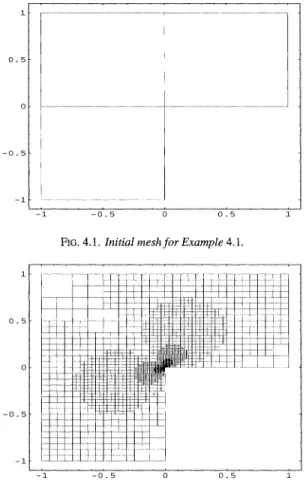
Figure4.1 is a giveninitial meshon the domain. Theadaptive computation shown in Fig. 4.2 is very similar to those using the code FEARS (finite element adaptive research

solver);

see,e.g., [6]. Our approachhoweveris muchsimplerin terms ofimplementing the error indicators. Dependingon the modelproblem, the location ofsingularity, the quantity ofinterest (displacement, stress,etc.), and the spectralorder of the

FE,

different extraction expressions for anauxiliary problemassociatedwith themodelproblem should be chosen

accordinglyforBabugka-Millerindicators; see[6]for more details. Ourerror indicators arenot confinedbythe aboveeffects;namely,oursdonotdependonsingularityandspectralorderand there arenoauxiliaryproblems. In fact,basedonthe ideas in thepresent paper,weareableto

developaverygeneraland robust code whichwecallAdaptC++. So far,wehavesuccessfully

testedourcode forlinearelasticityproblems, mixed-type problems,flows inporousmedia, obstacleproblems,Navier-Stokesequations, and semiconductor device simulationwith

FE,

FV,

andleast-squares

FE

methods.

Among

otherthings, one of itsadvantageousfeaturesis thesimplicityinimplementingthe error indicators which disregardinputmodelproblemsand seeonlyaverygeneral settingof linear and bilinear forms andboundaryconditions. Fromthe

user’s

viewpoint,use ofthecode is evensimplerpartlyduetothe refinement scheme and the object-oriented programminglanguage. All numerical datapresentedin this sectionexcept that inExample4.2 wereproduced by AdaptC++.

Tables4.1 and 4.2show thatadaptive computationsareclearly superiortouniformmesh reductions.Forinstance, ifatolerance isset to3 %of the relative error(r.e. Illelll the uniform

approach requires over 10 times the degrees offreedom

(DOF)

of the adaptive approach. Also, theeffectivity indices 0 show reliableerrorestimatorsfor both uniform and adaptive approximations.

-o.5;

-I -0.5 0 0.5 1

FIG.4.1. Initial mesh_forExample 4.1.

o.

-o 5

-i -0.5 0.5 1

FIG. 4.2. Adaptivefinalmesh(FEM)forExample4.1.

TABLE4.1

Example 4.1 usinguniformmeshes(FEM).

DOF Illelll r.e. 0 8

-0.284368

0.210 0.732 21 0.196695 0.145 0.801 65 0.128699 0.095 0.821 225 0.082777 0.061 0.830 833 0.052781 0.039 0.835 3201 0.033493 0.025 0.837

Example4.2. The discussions in

_3.2

are illustratedbythe nonlinearboundary value

problem

-Au=le

u,

u=u(x,y) (x,y) 6

f2=(O, 1)

x(O, 1),

(4.3)

u=O on o’3. The weak formulation of

(4.3)

isgivenas

(4.4)

(F(u,X), v).=

f.(.xux

-’-blyl)y

-)eUv)dxdy

=0 Vv e

_H(fl)

and we assumethat) _e

_R1,

whichmeansthat the solutions of

(4.4)

formaone-dimensional manifoldM.

TABLE4.2

Example4.1 using adaptive meshes(FEM).

DOF 8 21 34 53 78 119 301 469 765 1024 1847 Illelll r.e. 0 0.284368 0.210 0.732 0.196695 0.145 0.801 0.135229 0.100 0.849 0.096849 0.071 0.869 0.072604 0.053 0.877 0.054446 0.040 0.905 0.031254 0.023 0.945 0.024136 0.017 0.957 0.018578 0.013 0.966 0.010675 0.011 0.973 0.011501 0.009 0.980

Weuse auniformmesh,

T,

of 16biquadraticelements on f2. Forthecomputationof the one-dimensional solution manifold

Ms

of the discretizedproblem,a continuation

process

(PITCON

[23])

is applied starting from

(u,

;s

)

(0, 0), and ouraim is to determine a

posterioriestimatesof the error betweenM and

_Ms

atallcomputedsolutions (Us, ,ks)

Ms.

Inline with

(3.15)

and (3.16),the linearizedproblemat (Us,)s)

Ms

is to determine

(w,/z)

H

(f2) xA such that

(4.5)

fo

[11)x13

x -1I-Wyl)y

)seU"wv

+

eU#v]

dxdy

fa(UhxVx

+

blhyl)y-

)seU"v)dxdy Yv

6

Hd(f2),

(4.6)

((w, tz),

ts)

=0.

As

noted,the

ts

arechosen as normalizedtangentvectorson

_Ms

at

(us,)s).

Suchtangent

vectors are available ateach step of the continuationprocess and hence theequation

(4.6)

involves little additionalcomputationalcost.

For

local solutions each one, Z" ]", of the 16 elements of f2 is divided into m

(k

₊

1)2

biquadraticsubelements withk 1,4. That meansthaton eachsubelement,rij,

16, j 1 m,abubble-shapedfunction

l[rij

(X, y)isconstructed via themapping

of theshapefunction

1/t(,

1])

(1

2)(1

1]2

defined onthe reference element.

We

thus have

_S(ri)

_{span{Ttij}jm=l}

C

H(ri)

for each element_ri 6

7"

and hence

S-

C

Hd

(f2)is aconforming

FE

subspace. The more subelements areused,the moreaccurateauxiliarycondition

(4.6)

becomes and a betterqualityestimator canbe obtained.

Theresultingerrorestimates are shown in.Table4.3, where

_IwL

denotes thecomputed

error normsfor thetwo casesof k. Thecomputationsarevery

cost-effectiv

sinceeachlocal

probleminvolvesonlyafixednumberofdegreesof freedomdependingonthe value of k. The table also showsthat,asexpected,the estimated errorsvarysmoothly alongthe solutionpath

Ms

and show no sudden increases near the limitpoint) 6.804524.

As

mentionedearlier, if the natural coordinatesysteminducedbytheparameter space

A

ischosen,then weexpect

theresultingerror estimates

_Itbl

tobecomeunduly largenearthe limitpoint. This isindeed the case as thelast column of Table 4.3 shows.

At

the same time, it shouldbenotedthat the

computationalcostof thetwoapproachesispracticallyidentical.

TABLE4.3

Example4.2 usinguniformmeshes.

9

_{IIIwl III}

_IIIw4111

_II1111

5.907655 6.193552 6.434373 6.620862 6.745397 6.804524 6.800451 6.740221 6.633252 6.489009 6.328924 0.017914 0.018368 0.019144 0.020640 0.023317 0.027539 0.033461 0.041066 0.050283 0.061065 0.072480 0.019054 0.019562 0.020404 0.021986 0.024787 0.029185 0.035345 0.043255 0.052838 0.064041 0.075894 0.022905 0.024439 0.027792 0.041992 0.159595 0.176171 0.086353 0.069906 0.065171 0.065099 0.067672

Example4.3.

For

mixed-type

PDEs,

we considertheforward-backward heatequation

(4.7)

xt(x, t)

xx(X,

t)

f(x,

t)

V(x,

t)

f2 (-1,

1)

x (0, 1.),

b(_+l,t)--0 Yt 6[0,1],

(4.8)

4)

(x,

0)

0

Yx

6 [0, 1],

b(x,

1)=0

Yx

6[-1,0].

Note

that the equation changes typeasx changes sign in f2. There have been a number of

papers

addressingthis kindofmixed-typeheatequation;for further references see[5], [28].

For

ourcomputations,theexactsolution

_b

ischosen as

q(x, t) (x2

1)tz[(t

1)2-4x

2]

Vx

>

O,

[0, 1],

4)(x, t)

(x

2

1)(t

2

-4x2)(t

1)2

’x

< 0, [0, 1].

Denote

the

boundary

Of by

11

U...U176,

171

{(x,

t) x 6 [-1,0],

0},

172

{(x,

t) "x -1, 6 [0,1]},

173

{(x, t)’x

[-1, 0],

1},

174

{(x,

t)’x [0,1],

1},

175={(x,t)’x=l, t6[0,1]},

176

{(X,

t) x 6 [0,1],

0}.

By

achangeofdependentvariables,

II.

(Ul)--

(

e-O’lt

)

bl 2

e-O.ltx

(4.7)

can then beexpressedin symmetricpositiveform

(4.9)

Lu

A

lllxq--

Aztlt

-t--

A0u

f,

with

boundary

condition

(4.10)

Mu

"=

(/z

fl)u

0 (x, t) 6 0f2,

TABLE4.4

Example4.3: Boundarymatrices.

F1 0

o)

1-’3 ₀ 1"4 X 0 1"6 X 0

(;

o)

x 0

-x,

₀₎

0 0

Oot

-x

0)

0 0 0 0 0 x 0 TABLE4.5

Example4.3 using adaptive meshes.

DOF Illelll r.e. 0 20 1.310 0.804 1.035 72 0.344 0.211 0.985 156 0.155 0.096 0.972 272 0.087 0.054 0.966 420 0.056 0.034 0.963 600 0.039 0.024 0.961 812 0.029 0.017 0.961 where

()

-x -1

()()

x

(

e-O’ltf

₎

Ao=

O.Ix x f=

A

_{-1 0}

A

_{0 0 1 0}

/x,/3,

andMaregiven inTable 4.4.

It

canbereadilyshown that the system(4.9),

(4.10)

is symmetricpositive.

Theadjoint operator L*of

L

isdefinedby

L*v:=(

))Vx-( )vt+(O’lX+lx O1)v.

Now,

the weak formulationcorrespondingto

(3.23)

for

(4.7),

(4.8)

iscomplete.

For

FE

approximationof(3.23),a uniformmesh is introduced onf2 and bilinear elements areused. Onthe otherhand,thebubble-shapedfunctions

(4.11)

!/r(:, r/)

:(1

:2)(1/4

:Z)r/(1 -/72)(1/4

r]

2)

areusedtodefine

_(Sr)2.

Theeffectivityof error estimatesusing

(3.24)

isshown inTable4.5.

In

view of error equations

(3.5)

and

(3.24),

the calculation oferror indicators for the

present example proceedsinasimilarwayasthat ofExample4.1exceptthat we nowhave,in eachelement,a2 x 2systeminducedby

(3.24)

andbythecomplementaryfunctions

(4.11)

for

thevector-valued functions.

However,

bythenatureof symmetricpositivelinear differential

equations,the bilinear form associated with thesystemis coerciveonlyinthe

L2

norm

instead of in the usualH norm forelliptic problems.

Hence,

there is noequivalenceof theenergy

TABIF4.6

Example4.4 using adaptive meshes.

DoF

Illelll e. 0 32 0.0223

’0.1930

0.890 92 0.0117 0.1015 0.956 345 0.0053 0.0462 0.958 1489 0.0024 0.0211 0.980 5156 0.0012 0.0108 0.986 6833 0.0011 0.0096 0.987

normfound inellipticproblems. Ournumericalexperiencehas shown that thequadraticorder of thecomplementarybasis functions used as inExample4.1 gives ratherpessimistic error estimates. Theonly remedy to this difficulty seems tobe to usehigher order

(Sr)

2,

e.g.,

(4.11). Note

that this willnotcause morecomputationalcost, infact, thecost isalmost the same aswhen lowerorders are used. Apparently,the aposteriorierroranalysisformixed-type

PDEs

remainslargelyto befurther investigated.

Example4.4. Ourerror estimatorsfor variationalinequalities

(2.3)

aretestedbythe model

problemgiven in[4]withthe convexsetK

{v(x,

y) H (f2) v(x, y) >0andv(x, y) g(x, y) on

0f2},

where fa (0,

₇₎

x(0, 1) and g is chosen so that we have theexactsolution

0, if

(X

-[-

1)2

..[_

y2

>_ 2,

u _{1 1 1}

ln{ (x

₊

1)

2

or

₂

2]

otherwise.

[(x

+

1)

2

₊

y2]

2 2

The bilinear and linear forms are definedby

B(u,

v) :=

f

Vu

Vv

dxdy,

F(v) :=

f

vdxdy. ALGORITHM.

1. Givenaninitialmesh

_fah

on

2. Constructaconvexset

_Ks

withlinearshapefunctionson

_f2h.

3.

Use

theGauss-Seidel-SORmethod 18]withthe relaxationparameterandthe rela-tive errorchosentobe 1.2 and 10

-6,

respectively,toobtainanapproximatesolution

us

Ks

of the minimizationproblem

(3.26).

4. Constructthecomplementaryconvex set

_Kc

"=

{w

S-

C HT-(f2)and w

>-Us},

where

_S-

isdefined via

(4.2).

5.

In

each elementri,usethe method in

Step

3 to solve thereducedproblem

(3.28)

for

Y

6

Kc’,

which involvesonlyfourequationswithfourunknowns,and then calculate

the error indicator?]i for that element. Calculatethe error estimator for Us. Ifr.e.

> 0.01 then refine allelements with_Oi _>

0.1tlmax,

t]max max/r]i andgoback to

Step

2,otherwisestop.

The numerical results are shown in Table 4.6.

Example 4.5.

To

compare

FV

and

FE

computations, we consideragainthe L-shaped problem

(4.1).

For

any particular (1-irregular) mesh, e.g., Fig. 4.3,onf2, the

FV

elementapproximation

of

(4.1)

istofindut, 6 Ssuch that

Out,

ds

O,

b B b

where the

FE

space Sis defined as inExample4.1.

Note

that the test functions defined on the volumes

_bi

B

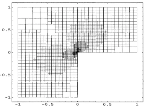
areequaltoone.

-i -0.5 0 0.5 1

FIG. 4.3. Adaptivefinalmesh(FVEM)forExample4.5. TABLE4.7

Example4.5 usinguniformmeshes(FVEM).

DOF Illelll r.e. 0 8 0.293127 0.217 0.748 21 0.199400 0.147 0.795 65 0.130269 0.096 0.817 225 0.083735 0.062 0.827 833 0.053375 0.039 0.832 TABLE4.8

Example4.5usingadaptive meshes(FVEM).

DOF _Illelll r.e. 0 8 0.293127 0.217 0.748 21 0.199400 0.147 0.795 34 0.136928 0.101 0.852 53 0.098177 0.072 0.874 78 0.073441 0.054 0.884 119 0.055017 0.041 0.910 188 0.041540 0.031 0.930 301 0.031497 0.023 0.947 459 0.024512 0.018 0.960 749 0.018927 0.014 0.965 1188 0.014646 0.011 0.973 1801 0.011699 0.009 0.979

CorrespondingtoTables4.1and 4.2, the data of the

FV

computationsare shown inTables 4.7 and 4.8,respectively. The finaladaptivemesh isshown inFig.4.3.

Acknowledgment. Theauthor would liketoexpresshisgratitudetothe referees formany

valuablecomments onthepaper.

REFERENCES

S.ADJERIDANDJ.E.FLAHERTY,Second-orderfiniteelement approximations anda posteriori error estimation

fortwo-dimensional parabolic systems,Numer.Math.,53(1988),pp.183-198.

[2] S. ADJERID, J. E. FLAHERTY,ANDY. J. WANG, Aposteriorierrorestimation withfiniteelementmethods_oflines forone-dimensional parabolic systems,Numer.Math., 65(1993), pp. 1-21.

[3] M. AINSWORTHANDJ. T. ODEN, A_unifiedapproachtoaposteriorierrorestimationusing element residual methods,Numer.Math., 65(1993), pp.23-50.

[4] M. AINSWORTH, J. T. ODEN,ANDC. Y.LEE,Localaposteriorierror estimators_forvariationalinequalities, Numer.Methods Partial Differential Equations, 9(1993), pp.23-33.

[5] A. K.AzIzANDJ.-L. LIU,Aweighted least squares methodforthe_{backward-forward}heat equation,SIAM J. Numer.Anal., 28(1991),pp. 156-167.

[6] I. BABUKAANDA.MILLER,The post-processingapproachinthefiniteelementmethods,Part1: Calculation

ofdisplacements,stressesand other higher derivatives_ofthe displacements,Internat. J. Numer.Methods

Engrg.,20(1984),pp. 1085-1109;Part2: Thecalculation_ofstressintensityfactors, Internat. J. Numer. MethodsEngrg., 20(1984), pp. 1111-1129; Part3: Aposteriorierror estimatesand adaptive mesh

selection,Internat. J.Numer.MethodsEngrg.,20(1984), pp.2311-2324.

[7] I.BABUgKAANDW. C. RHEINBOLDT, Errorestimates_foradaptivefiniteelement computations,SIAM J. Numer. Anal., 15(1978), pp.736-754.

[8] I. BABUKAANDD.Yu,Asymptoticallyexactaposteriorierrorestimator_forbi-quadratic elements, Finite ElementsAnal. Design, 3(1987),pp. 341-354.

[9] EL. BAEHMANN, M. S. SHEPHARD,ANDJ.E.FLAHERTY, Aposteriorierror estimation_fortriangular and tetrahedral quadratic elements usinginteriorresiduals,Internat. J. Numer.MethodsEngrg.,34(1992), pp.979-996.

[10] R. E. BANKANDD. J. ROSE, Someerror estimates_fortheboxmethod,SIAMJ.Numer.Anal., 24(1987), pp.777-787.

11] R.E. BANKANDA. WEISEP,, Someaposteriorierrorestimators_forelliptic partialdifferentialequations,Math. Comp.,44(1985), pp. 283-301.

[12] Z. CAI, Onthe_finitevolume elementmethod,Numer.Math., 58(1991), pp.713-735.

13] P.G. CIA,LET,TheFiniteElement Method_forElliptic Problems, North-Holland,NewYork, 1980.

14] L. DEMKOWICZ, J. T. ODEN, W. RACHOWICZ,ANDO.HARDY,Towardauniversalh-p adaptivefiniteelement strategy.Part1.Constrainedapproximation and datastructure,Comput.MethodsAppl.Mech.Engrg.,

77(1989), pp.79-11Z

[15] B. EDMANN, R. ROTZSCH,ANDF. BORNEMANN, KASADENumericalexperiments, TR91-1 Konrad-Zuse-ZentrumBerlin(ZIB),1991.

[16] R. S. FALK, Errorestimates_forthe approximation _ofaclass _ofvariational inequalities, Math. Comp., 28(1974), pp.963-971.

17] K.O. FmDCHS,Symmetric positivedifferentialequations,Comm.Pure Appl.Math., 11(1958),pp. 333-418. [18] R. GLOWNSKI, J. L. LIONS,ANDR.TP,flMOLIflRES, Numerical AnalysisofVariational Inequalities,

North-Holland, Amsterdam, 1981.

[19] D.W. KELLY,The self-equilibration_ofresidualsandcomplementaryaposteriorierror estimatesinthefinite

elementmethod,Internat. J. Numer.MethodsEngrg.,20(1984), pp.1491-1506.

[20] P. LESAINT,Finiteelement methodsforsymmetrichyperbolic equations,Numer.Math.,21(1973),pp. 244-255. [21] J.-L. LIUANDW. C. RHEINBOLDT,Aposteriorifiniteelementerror estimators_{forindefinite}ellipticboundary

valueproblems, Numer. Funct.Anal. Optim., 15(1994), pp.335-356.

[22] J.T. ODEN, L. DEMKOWICZ, W. RACHOWICZ,ANDT. A. WESTERMANN,Towardauniversalh-padaptivefinite

elementstrategy,Part2.Aposteriorierrorestimation,Comput.MethodsAppl.Mech.Engrg.,77(1989), pp. 113-180.

[23] W. C. RHEINBOLDT,Numerical Analysis_ofParametrizedNonlinear Equations,J.Wiley&Sons,NewYork, 1986.

[24] Onthe computation_ofmulti-dimensional solution_manifoldsofparametrized equations,Numer.Math., 53(1988), pp.165-181.

[25] W.C.RHEINBOLDTANDJ.-L.LIu,Aposteriorierrorestimates_forparametrizednonlinearequations, in Nonlin-earComputationalMechanics,EWriggers andW.Wagner,eds., Springer-Verlag, Berlin, 1991, pp. 31-46. [26] B.A.SA3OANDI.BABUKA,FiniteElement Analysis, Wiley,NewYork, 1991.

[27] T. TSUCHIYA, APrioriandAPosterioriErrorEstimates_ofFiniteElementSolutions_ofParametrizedNonlinear Equations, Ph.D. thesis,Dept.ofMath., Univ. ofMaryland, CollegePark,MD,1990.

[28] V.VANA3AANDR.B. KELLOGG,Iterativemethodsfora_{forward-backward}heat equation,SIAMJ.Numer. Anal., 27(1990), pp.622-635.

[29] O.C.ZIENKIEWICZANDJ. Z.ZHU,Asimpleerror estimatorand adaptiveprocedure_forpractical engineering analysis,Internat. J. Numer.MethodsEngrg.,24(1987), pp.337-357.