量子力學在動量空間的表象及其在鋰原子的強場游離之應用

國

立

交

通

大

學

物理研究所

博 士

論

文

量子力學在動量空間的表象及其在鋰原子的強場游離之應用

Momentum Representation in Quantum Mechanics with Application to

Strong-field Ionization of Lithium Atom

研 究 生：鄭世達

指導教授：江進福 教授

程思誠 教授

量子力學在動量空間的表象及其在鋰原子的強場游離之應用

Momentum Representation in Quantum Mechanics with Application to

Strong-field Ionization of Lithium Atom

研 究 生：鄭世達 Student：Shih-Da Jheng

指導教授：江進福 Advisor：Tsin-Fu Jiang

程思誠 Szu-Cheng Cheng

國 立 交 通 大 學

物理研究所

博 士 論 文

A Thesis

Submitted to Institute of Physics College of Science National Chiao Tung University in partial Fulfillment of the Requirements

for the Degree of Doctor of Philosophy

in

Physics

July 2013

Hsinchu, Taiwan, Republic of China

量 子 力 學 在 動 量 空 間 的 表 象 及 其 在 鋰 原 子 的 強 場 游 離 之 應 用

學生：鄭世達

指導教授：江進福

程思誠

國立交通大學物理研究所博士班

摘

要

我們建立了一套準確且有效率的方法，去解原子和雷射交互作用在動量空間

的表象的薛丁格方程式。我們的方法是建立在分離運算子方法(split-operator

method) 和 有 限 積 分 範 圍 的 蘭 迪 方 法 (Landé subtraction method with finite

integration limits)之上。我們測試了包含線性偏極脈衝、圓形偏極脈衝和長波長脈

衝的情況，我們的計算結果和其他計算方法得到的結果是一致的。我們也用有限

積分範圍的蘭迪方法去推廣李文斯坦模型(Lewenstein model)。接下來，我們應用

已建立的動量空間薛丁格方程式解法，去做鋰原子的強場游離的研究。在較低雷

射 強 度 的 區 域 ， 經 由 分 析 相 關 的 束 縛 態 被 佔 據 的 歷 史 和 將 光 電 子 頻 譜

(photoelectron spectra)分成奇數和偶數角動量部分，我們可以追溯出多光子游離

(multiphoton ionization)在光電子頻譜形成的峰點的來源。在較強雷射強度的區

域，我們指出了電子會穩定地停留在雷德堡態(Rydberg states)並解釋了為什麼游

離電子明顯集中到垂直於雷射偏極的方向。

ii

Momentum Representation in Quantum Mechanics

with Application to Strong-field Ionization of Lithium Atom

student：Shih-Da Jheng

Advisors：Dr. Tsin-Fu Jiang

Dr. Szu-Cheng Cheng

Institute of Physics

National Chiao Tung University

ABSTRACT

We developed an accurate as well as efficient scheme to solve time-dependent

Schrödinger equation in momentum space of an atom interacting with a laser pulse.

Our scheme is based on split-operator method in energy representation and Landé

subtraction method with finite integration limits. Cases of linearly polarized pulse,

circularly polarized pulse, and long wavelength pulses are tested. Our results agree

well with those from coordinate space calculations. We also apply the Landé

subtraction method with finite integration limits to generalize Lewenstein model. Next,

we use the developed P-space TDSE to study the strong-field ionization of a lithium

atom with a linearly polarized pulse. By analyzing the population history of relevant

bound states and separation the photoelectron spectra into odd and even angular

momentum parts, we can trace the origin of multiphoton ionization peaks in the lower

intensity regime. We point out the Rydberg stabilization and explain why the fan

structure becomes evident in the direction perpendicular to the polarization axis in the

higher intensity regime.

iii

誌

謝

兩年前，我從沒想過我可以在今年完成我的博士論文，甚至，我一度覺得我可能無法完成我的博士學位，而 現在竟然已經通過口試，在寫論文最後的誌謝部份了,到現在還是有點不可置信的感覺。首先，我要感謝我的指 導老師江進福老師和程思誠老師，兩位老師對研究都非常熱忱，在他們的指導下，我從完全不懂到可以掌握一個 領域的重點、學會研究過程中所需的技術並建立自己的工具、學著嚴謹地分析數據、還有從原本的不知所云到最 後漸漸可以將結果較清楚地呈現出來並發表。這些教導與訓練，不僅僅只是科學研究上的訓練，廣義上來說，這 是一個如何讓人可以將想法、創意具體實現的訓練過程，對於日後不論做什麼都有莫大的幫助。接著，感謝同研 究室的博士後研究員李漢傑博士，李博士對人熱心，對研究非常熱忱，受到他在研究上非常多的幫助。再來，感 謝在研究所一起打拼的同學、學弟，和大家一起吃飯聊天時，是苦悶的研究日子裡最輕鬆的時刻。最後要感謝我 的爸爸、媽媽、姊姊，謝謝你們的支持，讓我可以一直做我想做的事情。

Contents

1 Introduction 1

2 Methods 5

2.1 Time-dependent Schr¨odinger equation in momentum space

(P-space TDSE) . . . 6

2.2 Land´e subtraction method with finite integration limits . . . 10

2.3 Results of P-space TDSE . . . 16

2.3.1 Linear polarization case . . . 16

2.3.2 Elliptical polarization case . . . 19

2.4 Strong-field Approximation . . . 21

2.4.1 Keldysh-Faisal-Reiss (KFR) theory . . . 21

2.4.2 Lewenstein model . . . 22

2.4.3 Results . . . 23

3 Strong-field Ionization of a Lithium Atom 27 3.1 Compare with experimental results . . . 28

3.2 Features of strong-field ionization of a lithium atom . . . 34

3.3 Multiphoton ionization (MPI) . . . 41

3.3.1 Examination of the spectra for 30fs pulse . . . 43

3.3.2 Examination of the spectra for 10fs pulse . . . 44

3.4 Rydberg stabilization . . . 48

3.5 Fanlike structure in the direction perpendicular to the polarization axis . . 52

4 Conclusion 54 Bibliography 56 Appendix 61 .1 Dipole approximation, velocity gauge, length gauge, and Volkov state . . 61

List of Figures

2.1 Comparison of the numerical wave functions with the exact ones. . . 15 2.2 Electric field E(t) and vector potential A(t) of a five-cycles pulse. . . . . 16 2.3 Comparison of the photoelectron spectra for pmax = 100 and pmax = 10

of a hydrogen atom with a linear polarized laser pulse. . . 17 2.4 Comparison of the two-dimensional momentum distribution of the same

system as Fig. 2.3. . . 18 2.5 Comparison of the two-dimensional momentum distribution of a

hydro-gen atom with a linear polarized long wavelength laser pulse. . . 18 2.6 Comparison of the two-dimensional momentum distribution in the x-y

plane of a hydrogen atom with a circular polarized laser pulse. . . 20 2.7 Photoelectron spectra of the TDSE as well as two versions of SFA results

of a hydrogen atom with a linear polarized laser pulse. . . 24 2.8 Two-dimensional momentum distribution of TDSE and SFA1 of the same

system as Fig. 2.7. . . 26 2.9 Energy-angular momentum distribution of TDSE and SFA1 of the same

system as Fig. 2.7. . . 26 3.1 Iso-intensity surface plot of a laser-focal volume. . . 28 3.2 Two-dimensional momentum distribution of a lithium atom with a linear

polarized laser pulse for lower intensities. . . 30 3.3 Two-dimensional momentum distribution of a lithium atom with a linear

polarized laser pulse for higher intensities. . . 31 3.4 Photoelectron spectra of a lithium atom with a linear polarized laser pulse

for lower intensities. . . 32 3.5 Photoelectron spectra of a lithium atom with a linear polarized laser pulse

for higher intensities. . . 33 3.6 Energy levels of a lithium atom and the possible transition pathways. . . . 34 3.7 Two-dimensional momentum distribution of a lithium atom with a linear

3.8 Photoelectron spectra of a lithium atom with a linear polarized laser pulse with FWHM 30fs at a single peak intensity. . . 36 3.9 Two-dimensional momentum distribution of a lithium atom with a linear

polarized laser pulse with FWHM 10fs at single peak intensity. . . 37 3.10 Photoelectron spectra of a lithium atom with a linear polarized laser pulse

with FWHM 10fs at a single peak intensity. . . 38 3.11 Ionization probability vs Keldysh parameter γ. . . . 40 3.12 Schematic plot of the NRMPI and DRMPI processes. . . 41 3.13 Separation of the photoelectron spectrum into the even and odd angular

momentum parts. . . 43 3.14 Population history and photoelectron spectra of a lithium atom with a

linear polarized laser pulse with FWHM 30fs and 40× 1011_W/cm2_{. . . . 44} 3.15 Population history and photoelectron spectra of a lithium atom with a

linear polarized laser pulse with FWHM 10fs and 40× 1011_W/cm2_{. . . . 45} 3.16 transition from direct 4-photon ionization to direct 5-photon ionization. . 46 3.17 Peak-position of the highest peak vs laser intensity. . . 47 3.18 Schematic plot of the process of transition from direct 4-photon ionization

to direct 5-photon ionization. . . 49 3.19 Ionization probability, probability in low-lying states and probability in

Rydberg states vs Keldysh parameter γ. . . . 50 3.20 Ratio of the sum of the occupation probability of the Rydberg states (n ≥

5) to that of total bound states. . . 51 3.21 Two-dimensional momentum distribution of a lithium atom with a linear

polarized laser pulse for three different intensities in the higher intensity regime. . . 53

List of Tables

2.1 Numerical values of Ilfor l=0-19. [56]. . . 12

2.2 Comparison of eigenvalues and wave functions of a hydrogen atom be-tween ”Present” Land´e substraction method method and ”Ordinary” one for pmax = 100 a.u.. . . 13

Chapter 1

Introduction

Atomic ionization under strong laser field has been an attractive topic for decades. With the advance of the intense and short pulse laser technology, the study of the phenomena and corresponding applications of strong-field ionization continue to attract attention [1, 2]. Phenomena of an atom exposed to intense laser field include: multiphoton ionization (MPI), above-threshold ionization (ATI), tunneling ionization (TI), over-barrier ionization (OBI), and high-order harmonic generation (HHG).

MPI and ATI are associated processes. MPI is a process that a bound electron is ion-ized by absorbing enough photons successively to exceed the ionization potential. The ionized electron can continue to absorb more photons successively, then form evenly spaced multipeaks in the photoelectron spectra. The space between the two adjacent peaks is a photon energy. This is known as ATI [3, 4, 5, 6]. In a laser field, atomic po-tential can be suppressed by the laser field and form a popo-tential barrier. Then, an electron ionized by tunneling through the barrier is known as TI. OBI occurs if the laser intensity is so high that the peak of the potential barrier is lower than the ground state energy.

In the aspect of light, if an intense laser with frequency ω acts on atom samples, the spectra of the output light will contain odd multiple of ω. This is known as HHG. This phenomenon can be understood by the three-step model [7]: (i) an electron is ion-ized through tunneling, (ii) the ionion-ized electron is accelerated by the laser field, (iii) the electron is driven back by the laser field and recombines with the ion core. Then, emits high-order harmonic light and the cutoff is about Ip+ 3U p, where Ipis the ionization

po-tential of an atom and U p = I0/4ω2 is ponderomotive energy (or average kinetic energy) of a free electron in the laser field with intensity I0 and carrier frequency ω.

The regime of MPI and TI can be classified conveniently by Keldysh parameter [8, 9], which is the ratio of tunneling time to the period of the laser wave. It is given by

γ =

√

Ip

γ > 1, for lower laser intensity or larger frequency, is MPI regime. In this region,

photoelectron spectra are dominant by nonresonant multiphoton ionization (NRMPI) and dynamical resonant multiphoton ionization (DRMPI) [10]. Many experimental electron spectra, especially rare gas atoms, have been carefully studied in this regime [11, 12, 13, 14]. γ < 1, for higher intensity or smaller frequency, TI becomes dominant. This region has been investigated experimentally and theoretically but the interpretation of the data appears to be somewhat confusing so far [15, 16, 17, 18, 19, 20, 21]. Recent study in the mid-infrared regime reinforce such confusion [22, 23, 24, 25, 26, 27, 28]. And, to distin-guish the TI signature in the photoelectron spectra is still an interested topic [29, 30, 31]. By an intense laser field we mean the energy scale of laser-atom interaction is com-parable to the atomic binding energy. Therefore, perturbation theory is no longer valid. Nonperturbative treatment is needed. Two successful quantum mechanical theoretical tools that usually used to study the strong-field ionization are: numerical calculation of time-dependent Schr¨odinger equation (TDSE) and strong-field approximation (SFA) [7, 8, 32, 33]. Actually, SFA is still a perturbation theory but somewhat different from typical perturbation treatment. For initially bounded electron, laser field is treated as a perturbation. Once the electron is ionized, atomic potential become smaller for the dis-tant electron and thus is taken as a perturbation. SFA is a two-fold perturbation theory. However, SFA can only give a qualitative description, but is still useful due to its clear physical picture and easily handling. Numerical calculation of TDSE is more convincible, but it become computationally more challenging for higher laser intensity or longer pulse duration.

There are many methods for numerical calculation of TDSE, such as split-operator method [34], matrix iteration method [35, 36], Arnoldi-Lanczos method [37], Kramers-Henneberger like transform method [38, 39], using integration form [40, 41], and the time-dependent surface flux method [42] etc. In these methods, calculations are performed in the coordinate space (R-space). In the numerical calculation, a finite box will be set in the space. Due to the more spreading character of the ionized wave function in the R-space, it is easy to reach the boundary of the box and will then be reflected. To avoid reflection, a filter function is usually used at the boundary. Wave function will be filtered out when reaching the box boundary. In this way, some information in the wave function will be also filtered out. Especially at higher laser intensity, a more larger box will be required to retain more information in the wave function, so do the grid points. Hence, make the R-space TDSE difficult to perform accurately and efficiently.

Uncertainty principle tells us the more spreading ionized wave function in the R-space, the more it is localized in the P-space. If performing the calculation of TDSE in the p-space, it will be free from boundary reflection and the complete information will be

retained. Although it has such great advantage, it is difficult to obtain accurate results due to a singularity in the P-space Coulomb kernel. Recently developed P-space TDSE uses Land´e subtraction method to remove the singularity in the Coulomb kernel [43]. However, a larger upper bound pmax is still needed due to the typical usage of Land´e subtraction

method requiring a larger upper bound pmax for accuracy. This larger upper bound pmax

makes the time propagation of P-space TDSE not efficient.

In the first part of this thesis, we modify the Land´e subtraction method to be applicable in a smaller pmax, so called ”Land´e subtraction method with finite integration limits”.

Together with split-operator method in energy representation, we develop an accurate as well as efficient scheme to perform P-space TDSE [44]. In addition, we also apply the Land´e substraction method with finite integration limits to generalize the Lewenstein model by taking scattering process into account. Next, we apply the developed scheme to the study of strong-field ionization of a lithium atom [45].

Lithium atom is the third element in the periodic table. It has three electrons. The simplest atoms, hydrogen and helium, have been studied for long time, but the double ionization and correlation effect of the two electrons of a helium atom can be carefully studied only recently [46, 47, 48] due to the advance of GPU parallel calculation. And, the dynamics of a lithium atom under strong laser field become the next challenge and start to attract attention [49, 50, 51]. A recent paper reported experimental results to-gether with numerical TDSE calculations on the strong- field ionization of a lithium atom [51]. Two new techniques are used in the experiment: (1) experiment was performed in a magnetic-optical trap (MOT) and the thermal effect is small. (2) the reaction microscope technique was used to measure photoelectron spectra and the resolution is improved to

∼meV. In the experiment, a laser pulse with full width at half maximum (FWHM) 30fs

wavelength 785 nm and peak intensity in 1011 _{∼ 10}14_{were used. The classical estimation} by DC field, the laser intensity for OBI is I_P4/16Z2_{, where Z is atomic number and I}

P

is ionization potential. The OBI intensity for Li is 3.4× 1014W/cm2 hence γ = 3.7 for

wavelength 785 nm used in the experiment. This is in the MPI regime not in the TI regime as inert gas atoms. Therefore, with the lithium target under the laser parameters used in the experiment, MPI, OBI and TI regimes are all covered.

The two-dimensional momentum distributions and the photoelectron spectra were shown in the experimental paper. At lower intensity, the photoelectron spectra is orig-inated simply through nonresonant multiphoton ionization (NRMPI). At a little higher intensity, the intermediate bound states might be populated largely due to ac-Stark shift during pulse time and lead to a dynamical resonant multiphoton ionization (DRMPI) [10]. Complex peaks thus appear. For intensity higher than 8× 1012_{W/cm2, fanlike structure} appears. The long-range Coulomb interaction between the electron and its parent ion ,and

ponderomotive shift induced subpeaks explain this structure [52, 53, 54]. We also ob-served electron is distributed in the direction perpendicular to the polarization axis in the higher laser intensity regime. We perform calculations to examine the above mechanisms further.

Chapter 2

Methods

In the section 2.1, the scheme of the split-operator method in the energy representa-tion that we employ to solve the P-space time-dependent Schr¨odinger equarepresenta-tion (P-space TDSE) will be introduced. The most troublesome issue in this scheme is that there exist a singularity in the P-space Coulomb potential. In the section 2.2, we will introduce Land´e subtraction method which is a useful technique to remove such singularity. However, typical usage of this technique needs a larger upper bound in momentum pmaxto

guaran-tee the accuracy. This limitation make the application to the P-space TDSE not efficient. We modify the Land´e subtraction method to be applicable to a smaller momentum upper bound. Accuracy as well as efficiency in time propagation are thus improved. Results of P-space TDSE will be presented in the section 2.3. In the section 2.4, we first intro-duce two versions of strong field approximation which are very useful theoretical models to investigate the laser-atoms interaction under strong field. One is Keldysh-Faisal-Reiss (KFR) theory and the other is Lewenstein model. Then, we generalize the Lewenstein model to include scattering process by using Land´e subtraction method with finite inte-gration limits introduced in the section 2.2.

2.1

Time-dependent Schr¨odinger equation in momentum

space

(P-space TDSE)

The R-space TDSE of an atom interacting with laser field in the velocity gauge is given by i∂ ∂tΨ(r, t) = [H0+ Hi(t)] Ψ(r, t) (2.1) H0 = p2 2 + U (r) (2.2) Hi(t) = A(t)· p (2.3) A(t) =− ∫ t −∞E(t)dt (2.4)

where H0 is atomic Hamiltonian, U (r) is the atomic potential which only the motion of the outer most electron is considered (called single-active-electron approximation), Hiis

the laser-electron interaction in the velocity gauge and dipole approximation [Appendix], and E(t) and A(t) are electric field and its corresponding vector potential of the laser field. Atomic units (a.u.) are used throughout this thesis unless indicated otherwise. The P-space TDSE can be obtained by Fourier transformation [57, 58]:

i∂ ∂tΨ(p, t) = [H0+ Hi(t)] Ψ(p, t) (2.5) H0Ψ(p, t) = p2 2Ψ(p, t) + ∫ V (p, q)Ψ(q, t)dq (2.6) Hi(t) = A(t)· p (2.7) where Ψ(p, t) = 1 (2π)3/2 ∫ Ψ(r, t) exp(−ip · r)dr (2.8) V (p, q) = 1 (2π)3 ∫ U (r) exp[i(q− p) · r]dr (2.9)

We use second-order split-operator method to approach the time propagation of wave function.

The time propagation of the wave function from t to t+∆t can be divide into three steps: (i) free propagate for a half-time step ∆t/2

Ψ1(p, t + ∆t/2)≡ e−iH0∆t/2Ψ(p, t) (2.11) (ii) propagate under the influence of the laser field

Ψ2(p, t + ∆t/2)≡ e−iHi(t+∆t/2)∆tΨ1(p, t + ∆t/2) (2.12) (iii) free propagate for another half-time step ∆t/2

Ψ(p, t + ∆t)≡ e−iH0∆t/2_Ψ

2(p, t + ∆t/2) (2.13) In step (i), we first expand Ψ(p, t) and V (p, p′) in spherical harmonics Ylm(θ, ϕ). In

the following, we will only present linear polarized case, and can be generalized to any polarization easily under the same framework. For a linear polarized light, the system is azimuthal symmetric by assigning the polarization direction as the z axis. Therefore, only

m = 0 components will be involved.

Ψ(p, t) = l∑max l=0 gl(p, t)Yl0(θ, ϕ) (2.14) V (p, q) = 1 pq l∑max l=0 vl(p, q)Yl0(θ, ϕ)Yl0∗(θ′, ϕ′) (2.15)

where lmaxis the maximum number of partial wave and vl(p, q) will be expressed later in

Eq. (2.37). Then, Eq. (2.11) can be rewritten as: exp(−iH0∆t/2)Ψ(pi, θj, t) =

l∑max

l=0

[exp(−iH₀l∆t/2)gl(pi, t)]Yl0(cosθj) (2.16)

where H₀lΨ(p, t) = p 2 2 + ∫ vl(p, q)Ψ(q, t)q2dq (2.17)

is the radial part of the atomic Hamiltonian. Next, we represent the time evolution oper-ator Sl ≡ exp(−iH₀l∆t/2) in complete eigensets χkl(p) of the atomic Hamiltonian H0l. This scheme is the so called split-operator method in the energy representation [34]. And,

χkl(p) satisfies the following eigenvalue equation:

H_l0χkl(p) =

p2

2 χkl(p) +

∫

vl(p, q)χkl(q)q2dq = εklχkl(p) (2.18)

where εkl is the eigen energy corresponding to χkl(p). The time evolution of the radial

part of Eq. (2.16) can thus be expressed as: [exp(−iH₀l∆t/2)gl(p)]i =

N

∑

j=1

where

S_ijl =∑

k

χkl(pi)χkl(pj) exp(−iεkl∆t/2) (2.20)

Combining with angular part we get Ψ1(p, t): Ψ1(p, t + ∆t/2) =

l∑max

l=0

g(1)_l (p, t)Yl0(θ, ϕ) (2.21)

In step (ii), see Eq. (2.12), Hi(t + ∆t/2) = A(t + ∆t/2)p cos θ for linear polarized

light. Rather than coupling in p-subspace for each independent l through the convolution integration of the atomic potential in step (i), the cos θ in Hi couple the l-subspace for

each p independently here. We change the character of p and l and rewriting Eq. (2.21) as follow [43]:

Ψ1(p, t + ∆t/2) =

l∑max

l=0

g_p(1)(l, t)Yl0(θ, ϕ) (2.22)

And, we represent the time evolution operator exp[−iHi(t + ∆t/2)∆t] in the complete

sets χ(1)_ℓp(l) of the operator ˆK = cos θ in the{Yl0(θ, ϕ)} basis which satisfies

ˆ

Kχ(1)_ℓp(l) = λℓpχ

(1)

ℓp(l) (2.23)

where λℓpis the eigenvalue corresponding to χ

(1)

kl (p). Then, together with Eq. (2.22), Eq.

(2.12) can be rewritten as:

Ψ2(p, t + ∆t/2) = l∑max l=0 l∑max j=1 S_ijpg(1)_p (lj, t)Yl0(θ, ϕ) (2.24) where S_ijp =∑ ℓ χ(1)_ℓp(li)χ (1) ℓp(lj) exp(−iA(t + ∆t/2)pλℓp∆t) (2.25)

Step (iii) is just the same as step (i). After repeating step (i) again, the wave function Ψ(p, t + ∆t) is obtained.

After propagating to the end of the laser field at tf, we get a final time wave function

Ψ(tf). To extract the information of the ionized electron, we introduce a continuous state

projection operator: ˆ PC = ∑ Ei≥0 |χi⟩⟨χi| (2.26)

which is a summation of the outer product of eigenstates with positive eigen energy. Then, we can isolate the continuous part ΨC by operating ˆPC to the final time wave function

Ψ(tf).

ΨC = ˆPCΨ(tf) (2.27)

The momentum differential probability P distribution of the an ionized electron of energy E = p2_{/2 in the direction ˆpis given by}

∂3_P

∂3_p =|ΨC| 2

For a linear polarized light, the system is symmetric about the polarization axis. Two-dimensional momentum distribution can be obtained by integrated over the azimuthal angle ϕ about the polarization axis.

∂2_P ∂E∂θ = ∂3_P ∂3_p2πpsinθ (2.29) or ∂2_P ∂Esinθ∂θ = ∂3_P ∂3_p2πp (2.30) where θ is the angle between the polarization axis and the direction of the ionized photo-electron. The former form usually use to emphasize multiphoton ionization pattern [59] while latter one usually use to emphasize the electron distribution along the polarization direction [39, 43]. By integrating over θ in Eq. (2.29) and (2.30), we obtain the photo-electron spectra. ∂P ∂E = ∫ _∂2_P ∂E∂θdθ (2.31) or ∂P ∂E = ∫ _∂2_P ∂Esinθ∂θsinθdθ (2.32)

2.2

Land´e subtraction method with finite integration

lim-its

Since we represent the time evolution operator Sl ≡ exp(−iH₀l∆t/2) in complete eigensets of atomic Hamiltonian H₀l, solving the eigenvalue equation Eq. (2.18) is the central part of the P-space TDSE. Before proceeding, let’s examine the atomic potential first. In the single-active-electron approximation, only the motion of the outer most electron is con-sidered. The interaction between this electron and other inner shell electrons and atomic core can be modeled as a model potential [14, 60, 61]. The form of a model potential is not unique. We list one for example [61]:

V (r) =−1 r −

a1e−a2r+ a3re−a4r+ a5e−a6r

r (2.33)

When r → ∞, V (r) → −1/r which is the long-range Coulomb potential between the outer most electron and the ion core. The second short-range potential term account for the screened effect caused by other inner shell electrons where a′_is are variation

parame-ters to be optimized by fitting the energy levels from experiment data. This can be done by, for example, density functional calculations. Fourier transformation of this model potential is V (k) =− 1 2π2_k2 − 1 2π2 { a2 1 a2 2+ k2 + 2a3a4 a2 4+ k2 + a 2 5 a2 6+ k2 } (2.34) where k =|p − q|. Except the first long-range Coulomb potential term have a singularity at k = 0, others are well-behaved functions in the p-space and are easy to handle. The singularity in long-range Coulomb potential make it difficult to calculate eigenstates as well as eigenvalues accurately. To remove this singularity, Land´e subtraction technique has been proposed and the potential part of Eq. (2.18) is rewritten as [55]:

∫ vl(p, q)ψl(q, t)q2dq = Slψl(p, t) + ∫ vl(p, q) [ ψ(q, t)q2−ψ(p, t) Pl(z) p2 ] dq (2.35) where z = (p2_{+ q}2_{)/2pq, P}

l(z) is the Legendre polynomial, Slis defined as:

Sl≡ p2

∫ _v

l(p, q)

Pl(z)

dq (2.36) ,and vl(p, q) is the expansion of p-space Coulomb potential (−1/2π2k2) in {Ylm(θ, ϕ)}

basis, see Eq. (2.15), and has the following form:

vl(p, q) =−

1

πpqQl(

p2 _{+ q}2

Ql is Legendre function of the second kind and is defined as: Ql(z) = 1 2 ∫ 1 −1 1 z− xPl(x)dx (2.38)

when p = q, hence z = 1, vl(p, q) diverge because Ql(z) is divergent.

In Eq. (2.35), we just subtract the potential part of Eq. (2.18) by p2∫ vl(p, q)ψ(p,t)_P

l(z)dq

and add it back. By this trick, the terms in the square bracket tend to zero faster than the Coulomb potential vl(p, q) tends to infinity when q→ p and singularity is thus removed.

Hence we can redefine vl(p, q) for convenience [43]

vl(p, q) =    0 p = q Vl(p, q) p̸= q (2.39) Then, the eigenvalue equation Eq. (2.18) can be rewritten as:

[ p2 2 + Sl− ql(p) ] χkl(p) + ∫ Vl(p, q)χkl(q)q2dq = εklχkl(p) (2.40) where ql(p) = p2 ∫ _V l(p, q) Pl(z) dq (2.41) Now, we need to calculate Sland ql(p) in the Eq. (2.40). We rewrite Slas following:

Sl= p2 ∫ _v l(p, q) Pl(z) dq = −p π ∫ _Q l(z) qPl(z) dq =−pJl(p) (2.42) where Jl(p) is defined as Jl(p)≡ 1 π ∫ _Q l(z) qPl(z) dq (2.43) and the Legendre function of the second kind can be expressed alternatively as [62]

Ql(z) = 1 2Pl(z)ln z + 1 z− 1− Wl−1(z) (2.44) where Wl−1(z) = l ∑ k=1 1 kPk−1(z)Pl−k(z) (2.45)

Finally, Jl(p) has the form

Jl(p) = 1 2π ∫ lnz + 1 z− 1 dq q − 1 π ∫ _W l−1(z) Pl(z) dq q (2.46)

We should integral the two terms on the right hand side of Eq. (2.46) from 0 to∞ and these two terms can be calculated analytically. The first term is

1 2π ∫ _∞ 0 lnz + 1 z− 1 dq q = π 2 (2.47)

l Il l Il 0 0 10 1.487904713975699 1 1 11 1.495107943133761 2 1.224744871391589 12 1.501159656551487 3 1.322854905602328 13 1.506315483232877 4 1.377702237793946 14 1.510760615105643 5 1.412705039729489 15 1.514632500321632 6 1.436975208969198 16 1.518035295340011 7 1.454789864925959 17 1.521049367745399 8 1.468421032379340 18 1.523737720224722 9 1.479186912585977 19 1.526150439737141

Table 2.1: Numerical values of Ilfor l=0-19. [56].

We neglect the detail calculation of the second term and just define its as Il, so

Jl(p) =

π

2 − Il (2.48) Numerical values of Ilfor l = 0−19 are listed in Table 1 [56]. However, in the numerical

calculation, we can only set a finite upper bound pmax rather than ∞. Since Jl(p) is

obtained by integrating momentum q from 0 to∞, setting a larger upper bound pmax as

well as a large number of grid points for obtaining accurate eigenstates and eigenvalues is expected. As a result, the calculation is inefficient.

This problem can be cured by setting the integration upper bound of Jl(p) to a finite

value pmax. We denote the modified Jlby J f inite l (p). That is J_lf inite(p) = 1 2π ∫ _pmax 0 lnz + 1 z− 1 dq q − 1 π ∫ _pmax 0 Wl−1(z) Pl(z) dq q (2.49)

and the first term becomes 1 2π ∫ _pmax 0 lnz + 1 z− 1 dq q = π 2 − 2 π [ s + s 3 32 + s5 52 + s7 72 + ... ] (2.50) where s = p/pmax. The second term of J

f inite

l (p) can be calculated numerically. Together

with the numerical integration of ql(p) from 0 to pmax, the eigenvalue equation Eq. (2.40)

is ready to solve [63].

We map the P-space domain p∈ [0, pmax] to a new domain x∈ [−1, 1] by the

follow-ing mappfollow-ing function:

p(x) = L 1 + x

1− x + xm

(2.51) where L is mapping parameter and xm = 2L/pmax. The grid points are denser at small p

for smaller L. x is discretized by using Gauss-Lobatto quadrature where the N grid points

State E(nl)− exact ∆Φ

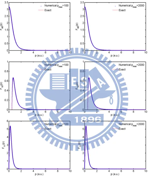
(nl) Present Ordinary Present Ordinary 1s 2s 3s 2p 3p 3d 1.76(-6) -6.45(-3) 2.75(-7) -1.61(-3) 1.24(-7) 7.16(-4) -1.56(-10) -4.14(-8) -8.75(-10) 1.83(-8) 2.38(-10) 2.38(-10) 6.90(-8) 2.45(-4) 6.88(-8) 4.25(-4) 6.88(-8) 6.17(-4) 1.01(-10) 1.34(-8) 6.46(-10) 1.84(-8) 4.21(-10) 4.22(-10) Table 2.2: Comparison of eigenvalues and wave functions of a hydrogen atom between ”Present” Land´e substraction method method with finite limits and the ”Ordinary” Land´e substraction method. [E(nl)-exact] is the deviation of energy levels for the first few low-lying states. ∆Φ is the root-mean-square deviation of the wave function. 2048 grid points and pmax = 100 a.u. are used. 1.76(−6) ≡ 1.76 × 10−6[44].

State E(nl)− exact ∆Φ

(nl) Present Ordinary Present Ordinary 1s 2s 3s 2p 3p 3d 7.77(-8) -3.18(-4) 6.55(-8) -7.96(-5) 6.25(-8) -3.53(-5) -1.78(-10) -4.95(-10) -9.45(-10) -1.06(-9) 3.86(-10) 2.70(-10) 5.99(-10) 1.22(-5) 1.01(-9) 2.11(-5) 1.41(-9) 3.07(-5) 4.39(-9) 1.90(-10) 6.85(-8) 7.69(-10) 7.66(-8) 5.58(-10) Table 2.3: The same as Table 2.3, but 2048 grid points and pmax = 2000 a.u. are used

[44].

In the Table 2.2 and 2.3, we present the energy deviation and root-mean-square de-viation of the radial wave functions between our numerical results and exact ones of a hydrogen atom. Root-mean-square deviation of the wave functions is defined as:

∆Φ = √ 1 N ∫ p2_dp|Φ(p) − Φ exact(p)|2 (2.52)

Φexact is the exact wave function of a hydrogen atom in the P-space. and first few

low-lying states are listed in the following [57, 58]:

F10(p) = 25/2 π 1 (p2_{+ 1)}2 (2.53) F20(p) = 32 √ π 4p2_{− 1} (4p2_{+ 1)}3 (2.54)

F21(p) = 128 √ 3π p (4p2_{+ 1)}3 (2.55) ”Ordinary” means the results of using typical Land´e subtraction method while ”Present” means the results of using Land´e subtraction method with finite integration limits. In Table 2.2, 2048 grid points and pmax = 100 a.u. are used. In Table 2.3, 2048 grid

points and pmax = 2000 a.u. are used. As mentioned above, typical Land´e subtraction

method needs a larger pmax to ensure the accuracy. Therefore, the ”Ordinary” results

for pmax = 2000 a.u. are more accurate than those for pmax = 100 a.u.. We can find

the ”Present” results improve the accuracy to several order than ”Ordinary” results at

pmax = 2000 a.u. as well as pmax = 100 a.u.. The results are more accurate at lager pmax

for both methods, especially for the s states. This is because P-space radial wave function tends to 1/pl+4 when p → ∞. So, s states (l = 0) are the most diffusive states, a larger

pmax is needed to reach higher accuracy. The improvement of the results to an acceptable

accuracy at small pmax by the ”Present” method will make the time propagation of TDSE

more efficient, as we will see in the next section.

In Fig. 2.1, we compare the numerical wave function for the ”Present” Land´e sub-straction method method with finite limits to exact ones for the first few low-lying states of a hydrogen atom. 2048 grid points are used and left column for pmax = 100 a.u. while

Figure 2.1: Comparison of the numerical wave functions of ”Present” Land´e substraction method method with finite limits with the exact ones for the first few low-lying states of a hydrogen atom. 2048 grid points are used and left column for pmax = 100 a.u. while

2.3

Results of P-space TDSE

In this section, we will present our P-space TDSE results and the emphasis will be put on the convergent test and calibration. The physics underlying laser-atom interaction under strong field will be discussed on the subject of the strong-field ionization of a lithium atom in the next chapter.

2.3.1

Linear polarization case

The linear polarized electric field E(t) of a laser pulse along the z axis can be described by

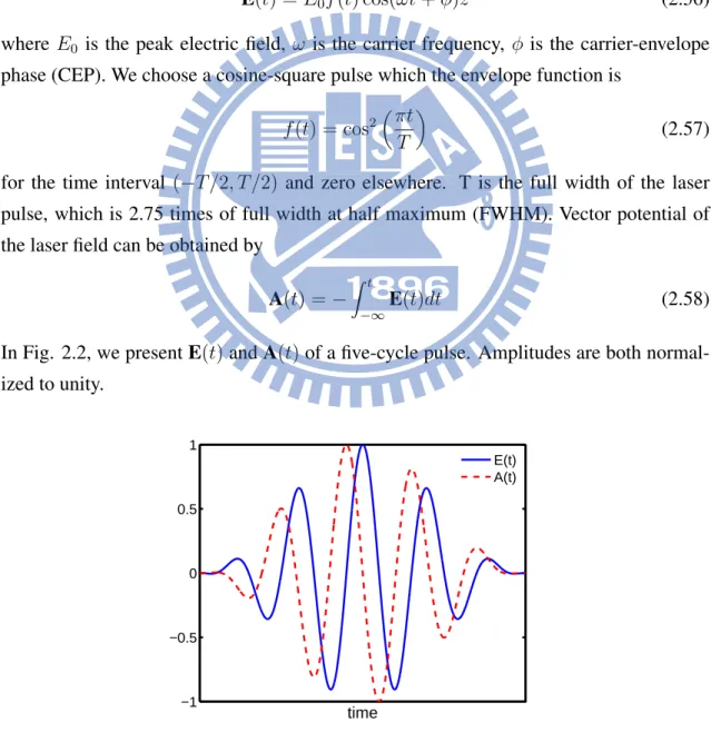
E(t) = E0f (t) cos(ωt + ϕ)ˆz (2.56) where E0 is the peak electric field, ω is the carrier frequency, ϕ is the carrier-envelope phase (CEP). We choose a cosine-square pulse which the envelope function is

f (t) = cos2

(_πt

T

)

(2.57) for the time interval (−T/2, T/2) and zero elsewhere. T is the full width of the laser pulse, which is 2.75 times of full width at half maximum (FWHM). Vector potential of the laser field can be obtained by

A(t) =−

∫ _t

−∞E(t)dt (2.58)

In Fig. 2.2, we present E(t) and A(t) of a five-cycle pulse. Amplitudes are both normal-ized to unity. −1 −0.5 0 0.5 1 time E(t) A(t)

Figure 2.2: Electric field E(t) and vector potential A(t) of a five-cycles pulse. Amplitudes are both normalized to unity.

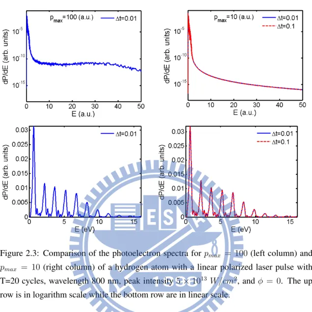
Figure 2.3: Comparison of the photoelectron spectra for pmax = 100 (left column) and

pmax = 10 (right column) of a hydrogen atom with a linear polarized laser pulse with

T=20 cycles, wavelength 800 nm, peak intensity 5× 1013 _W/cm2_{, and ϕ = 0. The up} row is in logarithm scale while the bottom row are in linear scale.

We consider a hydrogen atom under the laser pulse with T=20 cycles, wavelength 800 nm, peak intensity 5× 1013 _W/cm2_{, and ϕ = 0. In the calculation, we use 2048 grid} points, lmax = 14. In Fig. 2.3, we compare the P-space TDSE results for pmax = 100

a.u. (left column) and 10 a.u. (right column). The x-axis is plotted to 50 (a.u.) [1355 (e.v.)] in the up row while that is only plotted to 15 (e.v.) in the bottom row. At lower energy (bottom row), results are consistent between two different pmax. However, we

find that photoelectron spectra are not convergent yet after about 5 (a.u.) for the case of

pmax = 100 a.u. and time step ∆t = 0.01 a.u. (left top), since the probability of ionized

electron should be decay gradually toward high energy. But, for pmax = 10 a.u., the

photoelectron spectra is convergent very well even ∆t = 0.1 a.u. (right top). The case of ∆t = 0.1 a.u. only take 1/10 computation time than that of ∆t = 0.01 a.u.. As a result, the the Land´e subtraction method with finite integration limits improves the accuracy of the eigensets for a small pmax and thus make the P-space TDSE more efficiency.

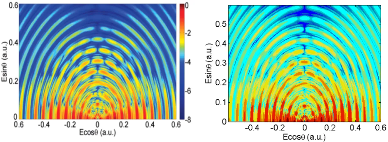
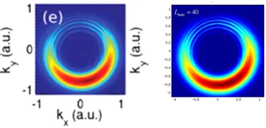
In Fig. 2.4, we present the two dimension momentum distribution of the ionized electron of the same system. Left sub-figure is from Ref. [43] and right sub-figure is our

Figure 2.4: Comparison of the two-dimensional momentum distribution of the same sys-tem as Fig. 2.3. Left sub-figure is from Ref. [43] and Right sub-figure is our result. results. Two results are consistent. We can find distinct ATI rings clearly.

Figure 2.5: Comparison of the two-dimensional momentum distribution of a hydrogen atom with a linear polarized laser pulse with T=10 cycles, wavelength 2000 nm, peak intensity 1× 1014 _W/cm2_{, and ϕ = 0. Left figure is from Ref. [39] and right} sub-figure is our result.

As another test, we consider a hydrogen atom under the laser pulse with T=10 cycles, wavelength 2000 nm, peak intensity 1× 1014 _W/cm2_{, and ϕ = 0. For a pulse in such} mid-infrared regime, the amplitude of free quiver motion of a electron in the laser field

α = E0/ω2 become larger. Therefore, a larger boundary box is expected in the R-space TDSE calculation and the computation time increases exponentially. However, there is no such problem in the P-space TDSE. In Fig. 2.5, we present the two dimension momentum distribution of the ionized electron. Left sub-figure is from Ref. [39] and right sub-figure is our results. In the calculation, we use 1024 grid points, lmax = 40, pmax = 10 a.u.,and

∆t = 0.05 a.u. Our result agree with theirs in the polarization direction (x axis) but lock of small node structures in their result. We comment that their angular resolution is not

good enough since only 32 angular grid points are used in their result, but we use 401 angular grid points.

2.3.2

Elliptical polarization case

The elliptically polarized vector potential A(t) of a laser pulse in the x-y plane is given by A = A0f (t)      cos(ωt + ϕ) cos(ϵ/2) sin(ωt + ϕ) sin(ϵ/2) 0      (2.59)

where A0is the peak amplitude, ω is the carrier frequency, ϕ is the carrier-envelope phase (CEP) and ϵ is the light ellipticity [ϵ = π/2 (0) for circular polarization (linear polarization along ˆx)]. We choose a cosine-square pulse the same as Eq. (2.53).

We consider a hydrogen atom under the laser pulse with T=3 cycles, wavelength 800 nm, peak intensity 1.06×1014_W/cm2_{, ϕ =}−π/2, and ϵ = π/2 (circular polarization). In the calculation, we use 256 grid points, lmax = 40, pmax = 100(a.u.), and ∆t = 0.1(a.u.).

In Fig. 2.6, we show the two-dimensional momentum distribution of ionized electron in the x-y plane (or θ = 0 plane). The left sub-figure is from Ref. [65]. Our result agree well with theirs.

For elliptical polarization case, all magnetic quantum number m will be involved. Given a lmax, the total angular subspace is (lmax + 1)2 which is an order greater than the

linear polarized case. Therefore, the calculation is much more expansive than the linear polarization case. In this case, we have used GPU parallel calculation (Tesla), but it still take about 29 hours.

Figure 2.6: Comparison of the two-dimensional momentum distribution in the x-y plane of a hydrogen atom with a circular polarized laser pulse with T=3 cycles, wavelength 800 nm, peak intensity 1.06× 1014W/cm2, and ϕ = −π/2. Left sub-figure is from Ref. [65] and right sub-figure is our result.

-2.4

Strong-field Approximation

Two versions of strong-field approximation will be introduced in this section. One is based on S-matrix theory which is named Keldysh-Faisal-Reiss (KFR) theory [8, 32, 33]. The other is based on an ansatz wave function which only the atomic ground state and continuous states are considered and first proposed by M. Lewenstein et al. [7].

2.4.1

Keldysh-Faisal-Reiss (KFR) theory

An exact expression for the probability amplitude of detecting an ionized electron with momentum p can be written as [59, 66]:

f (p) =−i

∫ _∞

−∞⟨Ψp|U(t, t ′_)H

i(t′)|Ψ0(t′)⟩ (2.60) where U (t, t′) is the time-evolution operator corresponding to total Hamiltonian H(t) =

H0 + Hi(t), H0 = p2/2 + V (r) is the atomic Hamiltonian, Hi = E(t)· r is the

laser-atom interaction in the length gauge, and Ψp(t) and Ψ0(t) are exact continuous state with moment p and ground state. U (t, t′) can be expansion as following:

U (t, t′) = UF(t, t′)− i

∫ _t

t′

dt′′UF(t, t′′)V U (t′′, t′) (2.61)

where UF(t, t′) is the time-evolution operator corresponding to Hamiltonian HF of a free

electron in the laser field, and

HF =

p2

2 + r· E (2.62) We use length gauge form here. The eigenstates of HF can be solved exactly and called

the Volkov states [Appendix]:

|χp⟩ = |p + A(t)⟩ exp[−iSp(t)] (2.63) where Sp(t) = 1 2 ∫ _∞ −∞dt ′_{[p + A(t}′_)]2 (2.64) and|k⟩ is plane wave:

⟨r|k⟩ = 1 (2π)3/2 exp(ik· r) (2.65) so ⟨r|k + A(t)⟩ = 1 (2π)3/2exp[i(k + A(t))· r] = 1 (2π)3/2exp(iA(t)· r) exp(ik · r) (2.66) where exp(iA(t)· r) is gauge factor in the length gauge. UF(t, t′) can be expanded with

the Volkov states:

UF(t, t′) =

∫

The key point of the SFA is to approximate the final exact continue state ⟨Ψp(t)| by the Volkov state⟨χp(t)| where the effect of atomic potential is considered small for an ionized electron in the strong field limit. Then, the ionization amplitude can be expressed as: f = f(1)+ f(2)+ ... (2.68) f(1) =−i ∫ _∞ −∞dt⟨χp(t)|Hi(t)|Ψ0(t)⟩ (2.69) f(2) =− ∫ _∞ −∞dt ∫ _∞ −∞dt ′∫ _{dk⟨χp(t)|V |χk(t)⟩⟨χk(t}′_)|H i(t′)|Ψ0(t′)⟩ (2.70)

f(1) is the first-order SFA (SFA1) and describe a direct ionization process induced by laser field. f(2) is the second-order SFA (SFA2), and describe rescattering of an ionized electron by the ion core.

We can find that (i) KRF theory is a two-fold perturbation theory. In writing down the exact expression Eq. (2.60), laser-atom interaction Hi is served as a perturbation.

Then, the total time evolution operator in Eq. (2.60) is expanded in atomic potential V(r), Eq. (2.61). This is because in the strong field regime, the laser-atom interaction energy becomes comparable to atomic potential energy. Therefore, one can’t just take laser-atom interaction as a perturbation as we usually do in the weak field regime. The physical idea underlying SFA is: For initially bounded electron, laser field is treated as a perturbation. Once the electron is ionized, atomic potential V(r) become smaller for the distant electron and thus is taken as a perturbation. (ii) After doing the expansion Eq. (2.61) and from Eq. (2.67), (and assuming the expansion is convergent), KRF theory only include the ground state and Volkov states, neglecting all other bound states. (iii) Depletion of the ground state is not consider in this theory.

2.4.2

Lewenstein model

Another version of SFA first proposed by M. Lewenstein et al. begins by making the following ansatz [7, 67]: |Ψ(r, t)⟩ = eiIPt [ a(t)|0⟩ + ∫ dp· b(p, t)|p + A(t)⟩ ] (2.71) where IP is ionization potential,|0⟩ and |p + A(t)⟩ are ground state and continuous states

with momentum p, similar to Eq. (2.66), A(t) is gauge factor, and a(t) and b(p, t) are occupation amplitudes to be determined. In this ansatz, only ground state and continuous states are considered. Further, continue states are approximated by plane wave

⟨r|k⟩ = 1

and the depletion of the ground state is neglected, which means a(t) ≈ 1. So far, all the approximations are similar to KFR theory. After substituting this ansatz into Schr¨odinger equation in length gauge:

i∂

∂tΨ(r, t) = p2

2 + V (r) + E(t)· r (2.73) and multiply ⟨p′′ + A(t)| from left hand side and integrate, we can obtain differential equation for b(p,t): i∂b(p, t) ∂t = [ (p + A(t))2 2 + Ip ] b(p, t) +⟨p + A(t)|Hi(t)|0⟩ + ∫ dp′b(p′, t)⟨p|V (r)|p′⟩ (2.74)

In the lowest order approximation of Lewenstein model, scattering term⟨p|V (r)|p′⟩ is neglected, and the differential equation can be integrated to give Eq. (2.69). Therefore, the lowest order approximation of Lewenstein model corresponds to the SFA1 of the KFR theory. Now, we recover scattering term by using the Land´e subtraction method with finite integration limits described in the section 2.2. Once the singularity in long range Coulomb potential is removed, the coupled-differential equation (coupling among all ps) can be solved using standard ODE solver. How does this result relate to KFR theory? If we expand KFR theory to the Nth-order in equation Eq. (2.61), together with Eq. (2.67) and Eq. (2.68), and assume the result has been convergent. Therefore, the terms after the Nth-order can be neglected. We can find that all these N terms we keep only include ground state and Volkov states (other bound states only exist in U (t, t′) which appears after the Nth-order in KFR theory and has been neglected due to convergent assumption.), just similar to the ansatz wave function proposed in the Lewenstein model Eq. (2.71) which only ground state and Volkov states are considered. So, the result of Lewenstein model with scattering term corresponds to summation of all N order of KFR theory since we didn’t do such an expansion as Eq. (2.61). Therefore, the Lewenstein model is a nonperturbative model.

2.4.3

Results

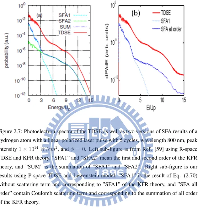
In Fig. 2.7, we show the photoelectron spectra of the TDSE as well as two versions of SFA results of hydrogen atom under a laser pulse with 5 cycles, wavelength 800 nm, peak intensity 1× 1014 W/cm2, and ϕ = 0. Left sub-figure is from Ref. [59] using R-space TDSE and KFR theory, while right sub-figure is our results using P-space TDSE and Lewenstein model. ”SFA1” and ”SFA2” in the left sub-figure means the first and second-order KFR theory respectively. ”SUM” means the summation of ”SFA1” and ”SFA2”. ”SFA1” in the right sub-figure means the results of solving Eq. (2.74) of Lewenstein

Figure 2.7: Photoelectron spectra of the TDSE as well as two versions of SFA results of a hydrogen atom with a linear polarized laser pulse with 5 cycles, wavelength 800 nm, peak intensity 1× 1014 W/cm2, and ϕ = 0. Left sub-figure is from Ref. [59] using R-space TDSE and KFR theory, ”SFA1” and ”SFA2” mean the first and second order of the KFR theory, and ”SUM” is the summation of ”SFA1” and ”SFA2”. Right sub-figure is our results using P-space TDSE and Lewenstein model, ”SFA1” is the result of Eq. (2.70) without scattering term and corresponding to ”SFA1” of the KFR theory, and ”SFA all order” contain Coulomb scattering term and corresponding to the summation of all order of the KFR theory.

model without the scattering term⟨p|V (r)|p′⟩ which is just the SFA1 in the KFR theory. ”SFA all order” is the result of solving Eq. (2.74). Since we don’t do any expansion, this results is corresponding the summation of all order of KFR theory. ”SUM” (blue-dotted line) in the left sub-figure is consistent with ”SFA all order” (blue-dotted line) in the right sub-figure except after electron energy greater then 12Up. The probability drop rapidly in

”SUM” while there exist another plateau in ”SFA all order”. Just as ”SFA2” contributes a plateau at 3-9Up, the plateau from 13Up in ”SFA all order” can be understood as the

contribution from the third and higher order terms corresponding to the KFR theory. After the third-order terms in the KFR theory, it is very difficult to evaluate due to at least 9-fold integration. Our P-space TDSE result consistent with ”SFA all order” (right sub-figure) but the R-space TDSE result exhibit a rapidly drop as ”SUM” after 12Up(left sub-figure).

are carried out. How about the drop in the R-space TDSE result? In the R-space TDSE calculation, a finite box in the coordinate space will be set. And the wave function will be filtered out when it reaches the box edge. More higher energy the electron possesses, more larger distant it can travel and hence be filtered out at the box edge. This should be the reason why the photoelectron spectra from R-space TDSE drop rapidly after 13Up.

We note that SFA only give a qualitative agreement of photoelectron spectra. ”SFA1” describe the tunneling process and contribute to the low energy part of photoelectron spec-tra (below 2Up). Coulomb scattering of the ionized electron and ion core contribute to the

higher energy plateau. However, the magnitude is smaller than the TDSE result by about 2 orders. The magnitude can be improved by forcing the final state to be orthonormal to the initial state which is called orthonormalized strong-field approximation (OSFA) [52, 68]. In Fig. 2.8, we present the two-dimensional momentum distribution of TDSE and SFA1 (Since Coulomb scattering wouldn’t affect low energy distribution in SFA, we only com-pare SFA1 to TDSE.). Up row are plotted according to Eq. (2.29) which emphasize electron distribution in the direction perpendicular to polarization axis while bottom row plotted according to Eq. (2.30) which emphasize that along the polarization axis. p_||and

pperp denote the momentum parallel and perpendicular to polarization axis respectively.

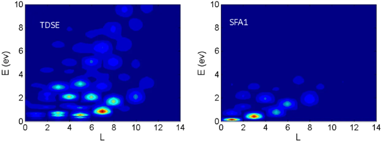
In Fig. 2.9, we present the energy-angular momentum distribution of TDSE and SFA1 which shows each angular momentum contribution to the photoelectron spectra. From Fig. 2.8 and 2.9, we find SFA give a totally different prediction from TDSE at low energy. Further, the breakdown of SFA is also pointed out in the recent interested mid-infrared regime [22, 23]. It is believed that the low energy electron would be affected by atomic potential significantly. The SFA can be improved by adding the Coulomb correction to Volkov wave function called Coulomb-Volkov wave function [69, 70].

Figure 2.8: Two-dimensional momentum distribution of TDSE and SFA1 of the same system as Fig. 2.7. Up row are plotted according to Eq. (2.29) which emphasize electron distribution in the direction perpendicular to polarization axis while bottom row plotted according to Eq. (2.30)which emphasize that along the polarization axis. p_|| and p_⊥ denote the momentum parallel and perpendicular to polarization axis, respectively.

Figure 2.9: Energy-angular momentum distribution of TDSE and SFA1 of the same sys-tem as Fig. 2.7 which shows each angular momentum contribution to the photoelectron spectra.

Chapter 3

Strong-field Ionization of a Lithium

Atom

In the section 3.1, we compare our calculation results to experimental results for cali-bration. To compare to experimental results, we need to average the signals of ionized electron from different atoms in the different region of the laser-focal volume (hence feel different laser intensity). Since the volume-averaged results contain so many signals, it is not convenient to analyze the underlying mechanism inside. In the section 3.2, we present the results at a single peak intensity (or without laser-focal volume average). In the sec-tion 3.3, we will discuss the multiphoton ionizasec-tion (MPI) at relatively small intensities, including nonresonant multiphoton ionization (NRMPI), dynamical resonant multipho-ton ionization (DRMPI), and ponderomotive shift. In the section 3.4, we will discuss the generation of Rydberg states in the lithium atom. In the section 3.5, we will discuss the fan structure in the direction perpendicular to polarization axis.

3.1

Compare with experimental results

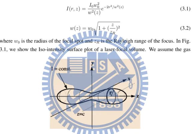
Before comparing to experimental results [51], we need to discuss laser-focal volume av-erage first. The focus of a actual laser beam is not a spot but has a volume. When we talk about the laser peak intensity I0of a laser beam, we always mean the value at the cental of the laser-focal volume. And, laser intensity decays gradually outward. The spatial distri-bution of the laser intensity can be formulated as Lorentzian in the propagation direction (z) and Gaussian in the transverse direction (ρ) [71, 72]:

I(r, z) = I0w 2 0 w2_(z)e −2r2_/w2_(z) (3.1) w(z) = w0 √ 1 + ( z zR )2 _(3.2) where w0 is the radius of the focal spot and zRis the Rayleigh range of the focus. In Fig.

3.1, we show the Iso-intensity surface plot of a laser-focal volume. We assume the gas

Figure 3.1: Iso-intensity surface plot of a laser-focal volume, z is the propagation direc-tion. This figure is from Ref. [72].

volume is filled over the laser-focal volume, then the ejected electron signals are the sum of electrons ionized from atom at different intensity region of the laser-focal volume. For a peak intensity I0, the ejected electron signals with momentum p is given by [71]:

S(P, I0) = D ∫ _I0 0 PI(P) ( −∂V ∂I ) dI (3.3) where D is the density of the target atoms, PI(P) is the ionization probability for a

par-ticular intensity I, and(−∂V_∂I)dI is the volume element between I and I+dI iso-intensity

surface. The volume element for the laser beam of Eq. (3.1) is given as

−∂V ∂I dI = πw3 0z0 3 1 I (_I 0 I + 2 ) √_I 0 I − 1dI (3.4)

The trapezoidal rule are used for the integration over intensity.

Now, we return to compare with experiment results. The experiment was carried out with a linear polarized laser pulse of wavelength 785nm, FWHM 30fs, and peak intensity

I0 ranging form 4× 1011W/cm2 (γ = 11.6) to 7× 1013W/cm2(γ = 0.8) which is from multiphoton ionization regime (γ > 1) to tunneling ionization regime (γ < 1).

We adopt the following model potential for a lithium atom [73].

V (r) =−1 r −

a1e−a2r+ a3re−a4r

r (3.5)

where a1 = 2, a2 = 3.395, a3 = 3.212, and a3 = 3.207. In our calculation, we use 1024 grid points, lmax = 14, ∆t = 0.2 (a.u.) and the laser-focal volume average is carried out

as: For peak intensity I0 = 4× 1011W/cm2and I0 = 8× 1111W/cm2, we integrate from 5%× I0 to I0 and ∆I = 0.2× 1011W/cm2. For peak intensity I0 = 7× 1013W/cm2, we integrate from 2.8%× I0to I0 and ∆I = 0.1× 1013W/cm2. All others are integrated from 5%× I0 to I0and ∆I = 0.1× 1012W/cm2.

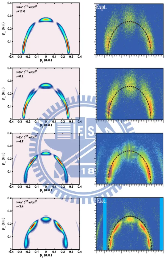
In Fig. 3.2 and 3.3, we show the two-dimensional momentum distribution of our results (left column) and experiment results (left column) for seven different peak inten-sity ranging from multiphoton ionization regime (γ > 1) to tunneling ionization regime (γ < 1). In Fig. 3.4 and 3.5, we show the photoelectron spectra with laser parameters corresponding to Fig. 3.2 and 3.3. Our results agree well with experiment results.

Figure 3.2: Two-dimensional momentum distribution of a lithium atom with a lin-ear polarized laser pulse with FWHM 30fs, wavelength 785nm, and peak intensity 4× 1011_W/cm2_{, 8× 10}11_W/cm2_{, 2× 10}12_W/cm2_{, and 4 × 10}12_W/cm2 _{(from up to} bottom). Left column is our results and right column is experimental results from Ref. [51]. p_|| and p_⊥ denote the momentum parallel and perpendicular to polarization axis, respectively.

Figure 3.3: The same as Fig. 3.2 but now laser peak intensity 8× 1012_W/cm2_{, 2×} 1013_W/cm2_{,and 7 × 10}13_W/cm2 _{(from up to bottom). Left column is our results and} right column is experimental results from Ref. [51]. p_|| and p_⊥ denote the momentum parallel and perpendicular to polarization axis, respectively.

Figure 3.4: Photoelectron spectra of a lithium atom with a linear polarized laser pulse with FWHM 30fs, wavelength 785nm, and peak intensity 4× 1011W/cm2, 8× 1011W/cm2, 2× 1012_W/cm2_{, and 4}× 1012_W/cm2 _{(from up to bottom). Left column is our results and} right column is experimental results from Ref. [51].

Figure 3.5: The same as Fig. 3.4 but now laser peak intensity 8× 1012_W/cm2_{, 2×} 1013_W/cm2_{,and 7 × 10}13_W/cm2 _{(from up to bottom). Left column is our results and} right column is experimental results from Ref. [51].

3.2

Features of strong-field ionization of a lithium atom

Since the volume-averaged results contain so many signals from different atoms which feel different laser intensity, it is not convenient to analyze the underlying mechanism inside. In this section and after, we will discuss the results at a single peak intensity with the same laser parameters as the experiment where wavelength 785nm, FWHM 30fs ,and intensity ranging form 4× 1011W/cm2 _{(γ = 11.6) to 7 × 10}13_W/cm2 _{(γ = 0.8). In} addition, we also study the short pulse cases with FWHM 10fs and 6fs.

Figure 3.6: Energy levels of a lithium atom and the possible transition pathways from ground state 2s induced by a laser pulse of wavelength 785nm (correspond to photon energy 1.57 eV). The length of a arrow represents a photon energy. This figure is from Ref. [51].

In Fig. 3.6, we show the energy level of a lithium atom and the possible transition path-ways from ground state 2s induced by a laser pulse of wavelength 785nm (corresponds to photon energy 1.57 eV). The length of a arrow means a photon energy. According to selection rule, only those transitions satisfying ∆l = ±1 are allowed for absorbing a photon. In this figure, we find that the electron cab be ionized by absorbing 4 photons. The first peak of ionized electron should be at ∼0.9 eV in energy (or 0.26 a.u. in mo-mentum|p|) and composed of l = 0, 2, and 4 partial waves. The most probably involved intermediate bound states are 2p, 3s, 4p, 4f, 5p, and 5f.

In Fig. 3.7, we present the two-dimensional momentum distribution without volume average for 30fs pulse. Let’s make some observation first. At smaller intensities, (a) and (b), we observe a 4-photon ionization ring. The number of nodes in the ring (except the two near x-axis) result from the zeros of Legendre polynomial Pl(cosθ) and thus indicate

Figure 3.7: Two-dimensional momentum distribution of a lithium atom with a lin-ear polarized laser pulse FWHM 30fs, wavelength 785nm, and peak intensity:(a)4× 1011W/cm2, (b)8 × 1011W/cm2, (c)2 × 1012W/cm2, (d)4 × 1012W/cm2, (e)8 × 1012_W/cm2_{, (f)2}×1013_W/cm2_{, and (g)7}×1013_W/cm2_{. p}

||and p⊥denote the momentum

Figure 3.8: Photoelectron spectra of a lithium atom with a linear polarized laser pulse FWHM 30fs, wavelength 785nm, and peak intensity:(a)4× 1011W/cm2_{, (b)8×} 1011_W/cm2_{, (c)2 × 10}12_W/cm2_{, (d)4 × 10}12_W/cm2_{, (e)8 × 10}12_W/cm2_{, (f)2 ×} 1013W/cm2, and (g)7× 1013W/cm2.

Figure 3.9: Two-dimensional momentum distribution of a lithium atom with a lin-ear polarized laser pulse FWHM 10fs, wavelength 785nm, and peak intensity:(a)4× 1011W/cm2, (b)8 × 1011W/cm2, (c)2 × 1012W/cm2, (d)4 × 1012W/cm2, (e)8 × 1012_W/cm2_{, (f)2}×1013_W/cm2_{, and (g)7}×1013_W/cm2_{. p}

||and p⊥denote the momentum

Figure 3.10: Photoelectron spectra of a lithium atom with a linear polarized laser pulse FWHM 10fs, wavelength 785nm, and peak intensity:(a)4× 1011W/cm2_{, (b)8×} 1011_W/cm2_{, (c)2 × 10}12_W/cm2_{, (d)4 × 10}12_W/cm2_{, (e)8 × 10}12_W/cm2_{, (f)2 ×} 1013W/cm2, and (g)7× 1013W/cm2.

which partial wave is dominant. In (a) and (b), the l = 2 partial wave is dominant, since there are two nodes in the ring. For (c), still a 4-photon ionization ring but l = 4 is dominant now. In addition, we find that the radius of the ring become smaller than (a) and (b). For (d), another ring appears inside the original one. From (e) to (g), the inner ring extend radially inward and resulting a fanlike structure. And, we find the electron is distributed to the direction perpendicular to the polarization axis gradually. This is strange since the motion of the electron will be driven by the laser field and there should be a more probability along the polarization axis.

In Fig. 3.8, we present the corresponding photoelectron spectra of Fig. 3.7. The first peak corresponds to the evident ring in Fig. 3.7. The following peak in (a), (b), and (c) is the associated 5-photon peak by absorbing one more photon from the former one hence differ by about a photon energy (1.57 eV). After (d), more peaks appear, where are they coming from?

In Fig. 3.9, we present the two-dimensional momentum distribution without volume average for 10fs pulse. At first glance, the features are similar to 30fs cases for (a) to (e) with a broader band, which is due to the uncertainty principle ∆E∆t > 1. The shorter (longer) the time duration of a pulse, the broader (narrower) the energy spectra. Inspection further, we find that the position of the double peaks in (d) is different from that in 30fs case. For (f) and (g), we find that two-dimensional momentum distribution is no loner symmetric. This can be understood as the contribution from tunneling ionization which is believed to be dominant at higher intensity (or smaller γ). Tunneling ionization is directional with the oscillation of a laser field and thus resulting asymmetric in the two-dimensional momentum distribution, especially for shorter pulse.

In Fig. 3.10, we present the corresponding photoelectron spectra of Fig. 3.9. The same as Fig. 3.8, the first peak corresponds to the evident ring in Fig. 3.9. and the two peaks in (a), (b), and (c) are associated 4-photon and 5-photon peaks. After (d), more peaks appear, but somewhat different from that in Fig. 3.8. Where are they coming from? In Fig. 3.11, we present the ionization probability vs Keldysh parameter (γ) for 6 fs, 10fs, and 30fs pulse. The vertical line at γ = 3.7 is the critical value of the classical OBI. It seems there is no dramatic behavior happening near this point. At γ = 2.5 and lower, the behavior of the ionization probability curves have significant changes for all three cases: For 30fs pulse, with the decrease of γ, we observe the ionization trapping and then suppression. For 10fs pulse, similar to 30fs initially, but the ionization probability recover and exhibits an oscillation in the end. For 6fs pulse, the ionization rate trends to smooth and also exhibit an oscillation in the end. Besides we also observe a ionization trapping around γ = 4.5 for 30fs pulse.

Figure 3.11: Ionization probability vs Keldysh parameter γ for 30fs, 10fs, and 6fs pulse. The vertical line at γ = 3.7 is the critical value of the classical OBI

In this section, we make an observation on the strong-field ionization of a lithium atom and leave several questions. In the following sections, we devote to answer these questions.