利用動態二進制轉譯技術改善微架構內快取記憶體模擬:個案研究

國立交通大學

資訊科學與工程研究所

碩 士 論 文

利用動態二進制轉譯技術

改善微架構內快取記憶體模擬:個案研究

Using DBT (Dynamic Binary Translation)

to improve performance of micro-architecture’s cache

simulations: a case study

研 究 生：陳君彥

指導教授：徐慰中 教授

利用動態二進制轉譯技術改善微架構內快取記憶體模擬:個案研究

Using DBT (Dynamic Binary Translation)

to improve performance of micro-architecture’s cache

simulations: a case study

研 究 生：陳君彥 Student：Chun-Yen Chen

指導教授：徐慰中 博士 Advisor：Dr. Wei-Chung Hsu

國 立 交 通 大 學

資 訊 科 學 與 工 程 研 究 所

碩 士 論 文

A Thesis

Submitted to Institute of Computer Science and Engineering College of Computer Science

National Chiao Tung University in partial Fulfillment of the Requirements

for the Degree of Master

in

Computer Science

May 2013

Hsinchu, Taiwan, Republic of China

i

利用動態二進制轉譯技術

改善微架構內快取記憶體模擬:個案研究

研究生：陳君彥

指導教授：徐慰中博士

國 立 交 通 大 學 資 訊 科 學 與 工 程 研 究 所 碩 士 班

摘

要

本篇論文是透過動態二進制轉譯相關技術嘗試改良微架構內快取記憶體模 擬之機制。有鑑於快取記憶體在微架構模擬中影響效能的權重，此實驗將關注在 如何改善其效能。其中將修改 SimpleScalar 並透過此一平台進行實驗。當測試 的程式，例如迴圈等重複執行且內含許多需存取記憶體的指令時，其中會產生許 多不必要的快取記憶體模擬。經由本實驗設計的方法，可偵測並進一步減少快取 記憶體模擬的次數以使整體效能提升。實驗結果顯示，改良後的 SimpleScalar 在執行快取記體憶模擬時的平均時間比起原本快上了 3.4~3.9 倍

ii

Using DBT (Dynamic Binary Translation)

to improve performance of micro-architecture’s cache

simulations: a case study

Student: Chun-Yen Chen

Advisor: Dr. Wei-Chung Hsu

Degree Program of Computer Science

National Chiao Tung University

ABSTRACT

This thesis uses DBT techniques to improve the performance of

micro-architecture’s cache mechanism. This study will focus on how to improve

cache simulation’s performance due to the cache importance in micro-architecture

simulations. We modified the SimpleScalar and ran the experiment on it. When

running the test codes with many memory reference instructions, such as loops,

repeatedly, there are many redundant cache simulations. By our experiment method,

these redundancies will be detected and the times of cache simulations will be

reduced. With the enhancement and associated optimization, we have observed

iii

誌

謝

感謝指導教授－徐慰中教授，給予我指導與幫助，從老師身上學到很多。不 僅是知識方面，最重要的是風範令人景仰。感謝口試委員：單智君教授、吳真貞 教授、楊武教授，在口試時，指明了學生在做研究時沒想清楚的部份以及寫作的 問題，讓我了解自己在研究上還有許多可改善的空間。 感謝實驗室詹雅淇、李柏舉同學，有他們的打氣和陪伴是一件很幸福的事。 感謝歐冠翬同學，在我遇到問題時，給了我許多的建議及幫助。感謝實驗室的大 家，真的覺得一起努力的感覺很棒。另外，感謝在口試當天幫忙的學弟劉冠宏、 傅勝余，使得口試得以進行得相當順利、流暢。 感謝交大資工系羽的學弟妹們，給了我很大的精神支撐，在這最後的一年， 謝謝你們。最後，謝謝家人的信任及鼓勵，還有情同兄弟的好室友黃致遠及莊柏 毅。

陳君彥

2013/05/17 NCTU (Lab. 446A)

iv

Table of Contents

摘 要... i ABSTRACT ... ii 誌 謝... iii Table of Contents ... iv List of Tables ... vi

List of Figures ... vii

I. Introduction ... 1 Motivating Example... 4 II. Background ... 9 2.1 Interpretation ... 9 2.2 Binary Translation ... 9 2.3 Micro-architecture Simulator ... 10 2.4 SimpleScalar ... 10

2.4.1 Sim-fast and sim-safe ... 13

2.4.2 Sim-profile ... 13

2.4.3 Sim-cache ... 14

2.4.4 Sim-outorder ... 15

III. Design and Implementation ... 18

3.1 Design Issues ... 18

3.2 Modify Cache Simulation Mechanism ... 19

3.3 Merge The Cache Simulations In The Same Cache ... 19

3.4 Address Overlapping Problem of Load/Store Instructions ... 23

IV. Experiments and Results ... 25

4.1 Experimental Environment ... 25 4.2 Case Studies ... 26 4.2.1 Array Addition ... 26 4.2.2 Memory Copy ... 26 4.2.3 Comparison ... 27 4.2.4 Linear Search ... 28 4.2.5 Bubble Sort ... 29 4.3 Preliminary Results ... 30

4.3.1 Array Initialization Problem ... 31

v

Cache miss rate ... 38 V. Conclusion and Future Work... 40 Reference ... 42

vi

List of Tables

Table 1 Code size of main functions in sim-outorder simulator ... 7

Table 2 Main components of SimpleScalar’s performance core ... 12

Table 3. Additional arguments of sim-cache level ... 14

Table 4 Read time of data cache simulation (in the main loop) ... 30

Table 5 Write time of data cache simulation (in the main loop) ... 30

Table 6 Read time of data cache simulation (Total) ... 31

vii

List of Figures

Figure 1 A simple C code example ... 5

Figure 2 Translated instructions: Interpreter vs. Micro-architecture

simulator (Add instruction with cache simulation only) ... 6

Figure 3 Code expansion problem ... 7

Figure 4 Simplescalar’s structure... 11

Figure 5 Simplescalar’s simulation levels ... 12

Figure 6 Set the cache hierarchy ... 15

Figure 7 Pipeline for sim-outorder ... 16

Figure 8 Code structure in sim-outorder ... 17

Figure 9 Execution flow of simplescalar ... 18

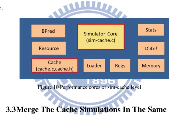
Figure 10 Performance cores of sim-cache level ... 19

Figure 11 The flowchart of implementation ... 20

Figure 12 Loop unrolling ... 21

Figure 13 Original implementation of instruction execution ... 22

Figure 14Modified implementation of instruction execution ... 23

Figure 15 Cache line’s status ... 23

Figure 16 Using clock gettime function to get the time of program

execution ... 25

Figure 17 Case: Array Addition ... 26

Figure 18 Case: Memory Copy ... 27

Figure 20 Case: Linear search ... 28

Figure 21 Case: Bubble Sort ... 29

Figure 22 code sequence of array initialization ... 32

Figure 23 Case : Array Addition (with default configuration of L1 data

cache) ... 33

Figure 24 Case : Memory Copy (with default configuration of L1 data

cache) ... 34

Figure 25 Case : Comparison (with default configuration of L1 data cache)

... 35

Figure 26 Case : Linear Search (with default configuration of L1 data

cache) ... 36

Figure 27 Case : Bubble Sort (with default configuration of L1 data cache)

... 37

viii

Figure 29 Data cache miss rate (Modified) ... 39

Figure 30 Example: Pipeline stages ... 40

1

I.

Introduction

In the computer engineering field, new ideas are often evaluated and verified by

simulations before actual implementations. A micro-architecture simulator simulates

the detailed implementations of a computer system implementation such as the

processor, the memory hierarchy, and sometimes, the memory interconnections and

buses. In the design of micro-architecture, simulations are frequently used to predict

the performance and tradeoffs are often made to fine tune the design. This process has

been very effective in reducing the cost of design, increasing the reliability and

performance of the implementation. In micro-architecture simulations, performance

critical components such as caches, register modules, out-of-order instruction issue

mechanisms, re-order buffers, branch predictors, load/store buffers are often modeled

in details. Usually, the more implementation details modeled, the more accurate the

predictions, but the slower the simulations. With all micro-architecture modules, the

cache hierarchy is one of the most importance, since it is not only performance critical,

but also frequently invoked by every memory reference instruction during the

program execution.

Traditional cache simulations are usually based on interpretation. It means that

each is interpreted and the memory operation involved is going through the cache

2

slow. Over the past many years, JIT(Just-In-Time Translation) techniques [1] have

been used to speed up the interpretation of bytecode, and DBT(Dynamic Binary

Translation) techniques have been adopted to speed up interpretation of executables

[2]. It is quite natural to question why such techniques were not used for speeding up

micro-architecture simulations.

This thesis investigates how DBT techniques may be used for fast

micro-architecture simulations. We started from cache simulations, but the idea could

be extended to other micro-architecture simulations such as the pipeline simulations

and the load/store buffer simulations. Although DBT is not a new technology, but it

has not been used effectively on micro-architecture simulations. DBT has been quite

successfully applied for function simulation, for example, most high performance

functional simulators, such as QEMU, Simics, Shade and so on, are based on DBT.

DBT turns interpretation into native code execution, for example, instead of

interpreting an “ADD” instruction, DBT translate this ADD instruction to an

equivalent native add instruction on the host machine, and the execution of this “ADD”

instruction is now emulated by executing the translated native instruction instead of

the slow process of interpretation. Translation needs to be done only once, since the

translated code will be stored in a code cache so that subsequent execution of the

3

applied to micro-architecture simulations, one challenge might emerge.

Micro-architecture simulations often involve lots of details to emulate. Those details

are often coded as functions and are called when the activities are involved in one

instruction emulation. If we translate all these activities into native code, the degree of

code expansion may degrade the simulation speed instead of making it go faster. We

will further discuss this impact in next paragraph and use some experimental data to

support this point. To avoid this code expansion dilemma, this study chooses a

selected area to apply the idea of DBT on micro-architecture simulation. In this study,

the simulation goes through the same components many times, for example, each

memory operation will call the cache simulator. We propose to have the dynamic

translator chooses some critical blocks of these components, applies optimizations to

get rid of redundancies, converts the selected blocks to native instructions, and stores

the translated code in the code cache for subsequent simulations.

There are significant redundancies exist among multiple load/store instructions.

Due to spatial locality, multiple load/stores are likely reference data located on the

same cache line. Instead of calling the cache simulation multiple times, the simulation

activities might be combined into one transaction. This is particularly useful for

frequently executed loops. According to the fact mentioned above, the DBT could

4

activities.

Before starting our work, a proper platform must be chosen. Simplescalar is a

well-known open source computer architecture/micro-architecture simulator, and it is

a set of tools that model a virtual computer system with CPU, caches and a memory

hierarchy. In year 2000, more than one third of all papers published in top computer

architecture conferences used the SimpleScalar tool sets to evaluate their designs. [3]

That is why we choose it for the investigation study.

The purpose of this study is to come up with a method for identifying these

redundancies and let a DBT to eliminate such redundancies via code transformations.

By eliminating the redundancies, the total time of data cache simulation, in this study,

would be decreased. We believe the same idea could also be applied to other

micro-architecture simulations. In our study, we modified the original sim-cache

simulator to include our proposed approach. Unmodified code will run as before, and

modified code will be executed as if the DBT has applied the transformation and

perform merged cache simulations.

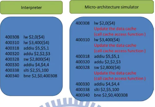
Motivating Example

In this paragraph, we will use real examples to point out the differences between

translating guest instructions to host instructions by interpretation or by DBT on

5

Use a short and simple code as example, as shown in Figure 1.

Figure 1 A simple C code example

In Figure 1, there are some arithmetic instructions in a loop. When we use

interpretation to emulate, the ADD and MUL instruction are emulated as a sequence

of instructions respectively, as shown in Figure 2. If we choose DBT to do the

emulation, the ADD and MUL instruction could be converted to native code, as

sample as one single native instruction, so the number of executed instructions in

emulation is much less than interpretation. Although the DBT is an effective way to

do emulation, but the speedup may not be realized when applied to micro-architecture

simulations. The reason is that micro-architecture simulators are not only translate

code like interpretation, but require many instructions to do the cache simulation,

6

Figure 2 Translated instructions: Interpreter vs. Micro-architecture simulator (Add

instruction with cache simulation only)

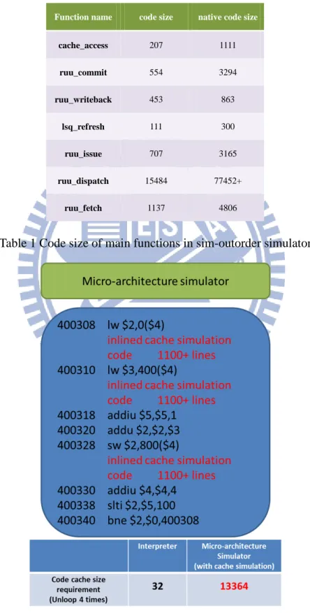
Code expansion problem

If we inline these function calls, the code expansion may slow down the program,

and the performance of simulation may be even less than the original one. Table 1

shows the code size of these functions. Even though the source C code is simple and

short, the translated code size of these functions is large. Based on this data, we take

Figure 2 and Figure 3 as examples; the number of instructions of micro-architecture

simulation (with cache simulation only) is about 3300 (according to Table1, each

cache access function translated to 1111 native instructions), it’s more than translated

code in interpretation. When the number of iteration is 100, the translated code size of

micro-architecture simulation with inlined cache simulation are much larger than

7

binary translation to translate the source instructions with native instructions, its

performance may be worse than original one.

Table 1 Code size of main functions in sim-outorder simulator

Figure 3 Code expansion problem

Function name code size native code size

cache_access 207 1111 ruu_commit 554 3294 ruu_writeback 453 863 lsq_refresh 111 300 ruu_issue 707 3165 ruu_dispatch 15484 77452+ ruu_fetch 1137 4806

8

In conclusion, instead of inline these functions, the better way to improve the

performance of micro-architecture simulation is to reduce the times of function calls.

Therefore, find a proper function to improve is important. Cache simulation is easier

and more potential than other functions to optimize.

The remainder of this thesis is as follows. In Chapter 2, we introduce the

background of this work. Chapter 3 shows the design and implementation of merged

cache simulations. In Chapter 4, we evaluate the performance of our design and

discuss the correctness and applicability of this approach. Chapter 5 summaries and

9

II. Background

In this chapter, we will introduce some important terms, which we could realize

and know their meanings in the following chapter. First, we discuss the translation

techniques between different ISAs and then explain what a micro-architecture

simulator need to do.

2.1 Interpretation

Interpretation is a straightforward emulation way. When a simulator uses

interpreter way from ISA1 to ISA2, it requires tens of native instructions to emulate

the execution of each source instructions.

2.2 Binary Translation

Binary Translation is a better way in emulation than interpretation, which makes

better performance during the translation. The reason is that binary translation

converts blocks of source instructions to native instructions and then stores these

native instructions in specific cache. Once the instructions are translated, we could use

and execute them repeatedly without doing the same translation again, it’s faster than

interpretation

There are two main types of binary translation, static and dynamic. Static binary

translation converts the guest binary code into code that runs on the target architecture

10

and code location problems. But, it can avoid some translation overhead at runtime.

Dynamic binary translation (DBT) takes a short sequence of code and then

translates it and caches the resulting sequence at runtime. Even though the overhead

of translation code is expensive, it significantly reduces the times of translation since

we can use the translated code in code cache repeatedly.

2.3 Micro-architecture Simulator

Differ with functional simulator, a micro-architecture simulator not only maintain

the program’s correctness but also go through the cache and use pipeline mechanism,

just like run a program in a true hardware environment. Therefore, the

micro-architecture simulator is more sophisticated than functional simulator and

implements more detail, so we need consider more problems if we want to modify it.

2.4 SimpleScalar

SimpleScalar is an open source micro-architecture simulator developed by Todd

Austin, which is a set of tools that model a virtual computer system with CPU, cache

and memory hierarchy. The early versions of tool set included contributions by Doug

Burger and Guri Sohi. [4] Today, SimpleScalar is developed and supported by

11

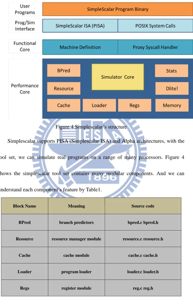
Figure 4 Simplescalar’s structure

Simplescalar supports PISA (Simplescalar ISA) and Alpha architectures, with the

tool set, we can simulate real programs on a range of many processors. Figure 4

shows the simplescalar tool set contains many modular components. And we can

understand each component’s feature by Table1.

Block Name Meaning Source code

BPred branch predictors bpred.c bpred.h

Resource resource manager module resource.c resource.h

Cache cache module cache.c cache.h

Loader program loader loader.c loader.h

12

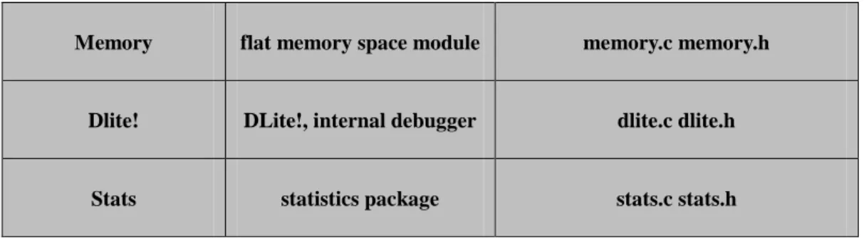
Memory flat memory space module memory.c memory.h

Dlite! DLite!, internal debugger dlite.c dlite.h

Stats statistics package stats.c stats.h

Table 2 Main components of SimpleScalar’s performance core

The above mentioned are lower layer (component layer) of simulator’s structure.

Now we introduce upper layer (simulator layer) of simulators. There are five levels in

Figure 5. It’s a trade-off between performance and detail. Each simulation level needs

corresponding performance core’s components to support it. In the following lines, we

will further describe the details of each simulation model.

13

2.4.1 Sim-fast and sim-safe

The sim-fast level resides in sim-fast.c .It executes each instruction serially.

Sim-fast is optimized for speed, and assumes no cache, instruction checking, and

doesn’t support for DLite!. DLite! is an internal in SimpleScalar tool set, which is a

lightweight debugger and could help us to trace the code structure.

Sim-safe is another version of sim-fast, and it also simulates functional

simulation, but checks for correct alignment and access permissions for each memory

reference. These two simulators cannot accept any additional command-line

arguments; both versions are very simple, therefore they are good starting points for

us to understand the internal works of the simulators.

2.4.2 Sim-profile

Just like its name, sim-profile can generate detailed program profiles on

instruction classes and addresses, text symbols, memory accesses, branches, and data

segment symbols. There are some extra options to show many different kinds of

profile information. For example, if we type the “-taddrprof” command-line argument

additionally, the terminal will show the execution profile by text address. In addition,

14

2.4.3 Sim-cache

Sim-cache is an ideal for fast simulation of cache and it generates one- and

two-level cache hierarchy statistics and profiles. In addition to universal arguments,

sim-cache accepts the arguments in Table3. The cache size is the product of <nsets>,

Table 3. Additional arguments of sim-cache level

Argument’s name Meaning

-cache:dl1/dl2 <config> level 1 / 2 data cache configuration

-cache:il1/il2 <config> level 1 instruction cache configuration

-tlb:dtlb <config> data TLB configuration

-tlb:itlb <config> instruction TLB configuration

-flush <config> flush caches on system calls

- icompress remaps 64-bit inst address to 32-bit equivalent

-pcstat <stat> record statistic<stat> by text address

<config> <name>:<nsets>:<bsize>:<assoc>:<repl>

<name> cache name

<nsets> number of sets

<bsize> block size

<assoc> associativity(number of “ways”)

15

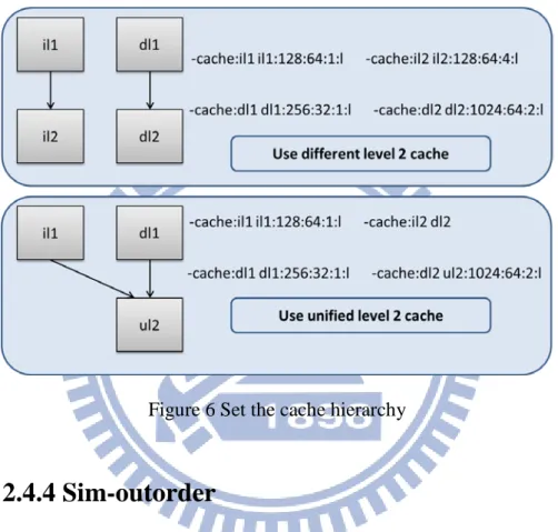
<bsize>, and<assoc>. As an example, “-cache:il1 il1:1024:32:2:l” will set a

2-way associative, 64K byte, level-1 instruction cache which uses LRU replacement

policy. To have a unified level in the hierarchy, “point” the instruction cache to the

name of the data cache in the corresponding level, as shown in Figure 6.

Figure 6 Set the cache hierarchy

2.4.4 Sim-outorder

Sim-outorder is the most complicated and detailed simulator, the main code file is

about 4000 lines. This simulator supports out-of-order issue and execution, based on

the Register Update Unit. The RUU renames the registers and hold the results, then

retires completed instructions in program order in each cycle. This simulator also uses

a load/store queue (LSQ unit). If the store is speculative, the values of store are placed

16

previous stores are known. Otherwise, it may generate cache misses.

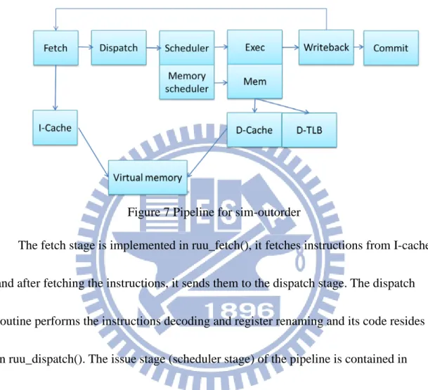
Figure 7 shows the pipeline of sim-outorder, there are six main stages for which

are fetch, dispatch, issue, execute, writeback and commit.

Figure 7 Pipeline for sim-outorder

The fetch stage is implemented in ruu_fetch(), it fetches instructions from I-cache

and after fetching the instructions, it sends them to the dispatch stage. The dispatch

routine performs the instructions decoding and register renaming and its code resides

in ruu_dispatch(). The issue stage (scheduler stage) of the pipeline is contained in

ruu_issue() and lsq_refresh(). These functions issue instruction to the functional units,

tracking register and memory dependencies. The execute stage is also maintained in

ruu_issue(). The routine receives as many ready instructions as possible from last

stage, and schedules writeback events by using the latency of the functional units. The

writeback stage is contained in ruu_writeback(), and it scans the event queue. When

17

instruction outputs to mark instructions that are dependent on the completed

instruction. This routine makes the dependent instruction as ready to issued when it

only waiting the completion. The ruu_commit() routine handles the instructions from

writeback stage that are ready to commit. It does committing instructions, updating of

the data caches and handling date TLB miss. When an instruction is committed, its

result is placed to the architected register file, and the RUU and LSQ states must be

updated.

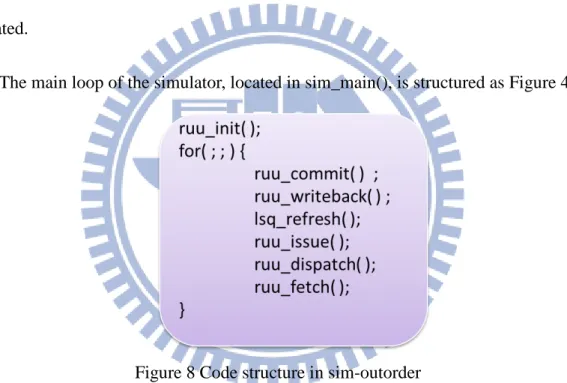
The main loop of the simulator, located in sim_main(), is structured as Figure 4.

Figure 8 Code structure in sim-outorder

As shown in Figure 8, the pipeline is executed reversely. By this method, the

18

III. Design and Implementation

3.1 Design Issues

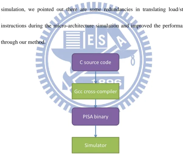
As shown in Figure 9, if we want to run a program in SimpleScalar’s instruction

set, it must be compiled to PISA binary first. Then the simulator can run this binary

code to help us analysis the cache line’s information, cache miss rate and load/store

instructions count etc... Since this report aims to reduce the overhead of cache

simulation, we pointed out there are some redundancies in translating load/store

instructions during the micro-architecture simulation and improved the performance

through our method.

19

3.2 Modify Cache Simulation Mechanism

As mentioned previously, this study aims to reduce the cache simulation’s time.

Therefore, we choose the sim-cache simulator to implement our method and modify

the cache mechanism in it. As shown in Figure 10, the simulator implements the way

of the cache simulation’s function call, it contained in sim-cache.c, and the cache

model resides in cache.c and cache.h. The above files are the target that we will focus

on.

Figure 10 Performance cores of sim-cache level

3.3 Merge The Cache Simulations In The Same

Cache

Sim-cache translates and executes the instructions serially. Since that, the same

translated code is executed repeatedly when the program has loops in it. Take forloop

as example, programmers usually use forloop to deal with computations, memory

copy, searching algorithm and string comparison. The data are stored continuously in

20

continuous. Each load or store instruction implicitly calls a cache access function to

handle the data cache simulation and the accessed locations are consecutive in this

situation. Based on this conclusion, we could merge the simulations into one when the

accessed cache blocks are in the same cache line.

The following steps are used to achieve our goal, as proposed in Figure 11.

Figure 11 The flowchart of implementation

First, we create some variables to record the old PC (program counter) and check

whether there is a loop or not during the simulation’s routine. If the value of old PC is

bigger than current PC, and the address of current PC is always equal to the one of

last comparison, the loop exists. Then record the instruction sequences between these

two program counters. After checking the continuity of memory addresses, the

21

cache line. Use the default configuration in sim-cache as example, the data cache line

size is 32 bytes, each load word instruction accesses 4bytes data from the data cache.

Therefore, the maximum number of unrolling is 8 in this case.

Loop unrolling is a loop transformation technique that attempts to upgrade a

program’s performance. After unrolling, the loop is expanded. There are repeat

instruction sequences in the unrolled loop, as shown in Figure 12.

Figure 12 Loop unrolling

The arrowed instructions is the same instruction in each loop iteration, these

instructions call the cache access function, accessing the data cache continuously after

unrolling the loop.

Now we can merge these simulations into one. In our modified routine, the first

load or store instruction calls a cache access function which accesses four times of

22

the original simulator’s routine uses switch statement and macro functions to do the

implementation of instruction execution. This switch statement uses an enumerated

type “op” which is passed as argument here and its value corresponds to opcode’s

name. SYMCAT is a macro function which combines the OP’s name and the string

‘IMPL’ to a macro function. Take lw (load word) instruction as example, the

SYMCAT returned a combined string “LW_IMPL”, it has been defined in the

“machine.def” and this function call multilevel macro calls to finish the instruction

execution.

Figure 13 Original implementation of instruction execution

Figure 14 shows a part of code of modified version of sim-cache simulator.

LW_CACHE_IMPL represents a multilevel path of optimized cache simulation, and

the LW_MEM_IMPL updates memory status but not goes through the data cache. The

branch flag is set to count the stall of load word instructions, because after merged the

23

Figure 14Modified implementation of instruction execution

Figure 15 shows the difference between original and modified way. In ideal

situation, the speedup of cache simulation time is 4.

Figure 15 Cache line’s status

3.4 Address Overlapping Problem of Load/Store

Instructions

In the above paragraph, we explain our method in detail. However, there is a big

24

addresses which be accessed by load/store instruction must be continuous first, so the

cache line’s value can be the same as the original one after executing the modified

routine. But there is a special case that the program will choose the original routine to

25

IV. Experiments and Results

In this chapter, the experimental result using different cases is shown. Each case’s

number of iteration is 10 to 100000 times; hence the result could show the

performance from small to large. We use SimpleScalar 3.0, SimpleScalar PISA GNU

GCC compiler and SimpleScalar PISA GNU binary utilities which are required for

users to use the PISA instruction set and build their own binaries.

4.1 Experimental Environment

Our experiments run on an Inter i5-760 @ 2.80GHz with 4GB RAM desktop

machine. The operating system is 32-bit Ubuntu 12.04 LTS. The test cases are

mentioned behind; these cases are compiled with –O3 flag by SimpleScalar compiler

tools that are based on GNU GCC. The program execution time is measured by

clock_gettime function. It is accurate to nanosecond that is more precise and proper

than the gettimeofday function, since the cache simulation time is usually hundreds of

nanoseconds. Figure 16 shows how to use this function to calculate the execution

time.

26

4.2 Case Studies

First, we will introduce some cases in a loop and implement our speedup methods

on them in this part and explain the common problems in these cases. Then explain

how to solve or avoid them.

4.2.1 Array Addition

As shown in Figure 17. This case is a simple add instruction in a loop. It loads

data from two addresses, then adds it and stores the result in another memory address.

Figure 17 Case: Array Addition

4.2.2 Memory Copy

In this case, we only copy the data from an address to another one. Since there is

one load and one store word instruction, the times of data cache access are two for

27

Figure 18 Case: Memory Copy

4.2.3 Comparison

It is a common case when we try to determine a variable’s value by a comparison.

Such as A equals B, A is greater than B and A is not equal to B etc… In Figure 19, we

make array c’s value 0 when the value of array a and b are equal, otherwise the value

of array c is 1. The lower right corner of Figure 19 shows the translated code, the first

and second line are normal load instructions, we could use our optimization on them,

but the store instructions in the following lines cannot be optimized. Since we don’t

know whether the comparison is taken or not, we cannot merge the cache simulation

28

Figure 19 Case: Comparison

4.2.4 Linear Search

This case is a very simple search method which we often used it to find specific

number in an array. All the value in array arr[] are produced randomly, so did the

value of “search”. After found the target number, this case set array arr2 and flag is 1.

29

4.2.5 Bubble Sort

This case is a bubble sort which works by comparing each element of the list with

the element next to it and then swapping them if required. Since this case uses a

comparison before swapping the array data, the sequence of translated code is similar

to comparison case one which is mentioned above. Figure 21 shows the source c code

and the translated code sequence of this case. There are two store word instructions

after branch equal instruction in the fourth line of translated code. When this branch is

taken, these store instructions have been jumped, therefore them cannot be optimized

by our implementation way. As expected, the performance gain may be lower than

array addition and memory copy and be close to comparison case.

30

4.3 Preliminary Results

This section shows the early result of our experimental method. We choose array

addition case to verify our method. Table 3 and 4 shows the read time and write time

of data cache simulation in the main optimal loop respectively. The ratio of original

version to modified one is about 3.3x to 3.8x, which means the speedup of data cache

simulation. It’s close to the theoretical value as mentioned previously.

Iteration times Original(nsec) Modified(nsec) Ratio

100 124508 32513 3.82

1000 12339431 333466 3.72

8000 10486522 3106978 3.38

Table 4 Read time of data cache simulation (in the main loop)

Iteration times Original(nsec) Modified(nsec) Ratio

100 63209 18015 3.51

1000 598556 179722 3.33

8000 5050219 1500883 3.36

Table 5 Write time of data cache simulation (in the main loop)

The following tables show the total time of data cache simulation with original

and modified version. As shown in Table5, the speedup is only about 1.5 and the

31

Iteration times Original(nsec) Modified(nsec) Ratio

100 457357 349692 1.31

1000 2779136 1830592 1.52

8000 21107228 13715219 1.54

Table 6 Read time of data cache simulation (Total)

Iteration times Original(nsec) Modified(nsec) Ratio

100 2485621 2407451 1.03

1000 3962573 3518010 1.12

8000 17512895 13812644 1.27

Table 7 Write time of data cache simulation (Total)

4.3.1 Array Initialization Problem

After profiling, we found the bottleneck of the total cache simulation. In these

test codes, the arrays are initialized before using. The compiler implicitly initializes

these arrays iteratively, just like copying memory data from an array to another one in

a forloop. Figure 22 shows the translated code sequence of array initialization. There

is a little different to those cases mentioned previously. The memory address is

continuously with load/store word instructions in each loop, so we don’t need to

unroll the loop to improve it. To reduce the total time of cache simulation, a feature

32

shown in Figure22, merging load’s cache simulation into one, so do store’s. Therefore

the total time of cache simulation is decreased significantly. In the next chapter, this

study will show the this optimization’s influence

Figure 21 code sequence of array initialization

4.4 Experiment Results

This section shows the final results of above cases. First we display the data of

each case in default of cache and make some explanations of these results, then

compare the performance of cache block size. After the performance issue, the

analyses of cache miss rate of each case are shown to ensure the correctness of our

modified version. Finally we briefly conclude the effect of our optimal method in

micro-architecture simulator’s cache.

33

default configuration (with 256 sets, 32 bytes for each block and the associative of set

is 1) and its size is 8KB. As the first case, we introduce the parts of this diagram in

detail. In the bottom of this diagram, the horizontal axis shows the number of loop

iterations and in the left of this figure, the vertical axis shows the ratio of original

Simplescalar’s data cache access time to modified versions. There are 4 columns in

fixed iterations of loop. The left hand side is the collections of read/write data in the

optimal scope and the right hand side is the collections of read/write data during the

whole program. This study will use the same format to perform the results in the

following figures.

Figure 22 Case : Array Addition (with default configuration of L1 data cache)

As shown in Figure23, the speedups are not consistent when the loop iteration’s

34

by experimental error. The largest test data displays the modified version’s speedup is

about 3.4x to 3.5x and the experimental results between the optimal loop and the

whole program are more and more closely when the iteration’s number goes from

small to big; in other words, the charts which consist of 4 columns are getting more

and more smoothly from left to right.

Figure 23 Case : Memory Copy (with default configuration of L1 data cache)

Figure 24 shows the case 2 results. The purple charts show the improved

performance of write data cache access during the whole program time. When the

iterations go from small to big, the dark red charts which mean the modified write

data cache performance of the optimal loop scope look like as the purple chart. And

the same phenomenon is shown in blue and green chart. It means that the results are

getting more stable of large test case. In conclusion, the speedup is about 3.3x to 3.5x

3.33 3.38 _3.21 3.35 _3.19 3.39 3.45 3.53 3.18 3.34 3.34 3.43 3.39 3.4 3.59 3.54 0 0.5 1 1.5 2 2.5 3 3.5 4 100 1000 10000 100000 Speedup

The number of loop iterations

Memory Copy

35

in the largest case.

Figure 24 Case : Comparison (with default configuration of L1 data cache)

In Figure 25, the blue charts are more evident than the others. The reason is that

the modified routine only change the load mechanism in the optimal loop and it

account for a small rate of the total load instructions. Therefore, the dark red charts

are all close to 1 because the write data cache mechanism is the same; and the green

charts grow slightly when the number of iterations changed from 100 to 100000.

There is only one kind of charts hasn’t be mentioned above – the purple charts. It

shows the total time of write data cache access is reduced, but it looks like

unreasonable since the write data cache efficiency in the optimal loop is almost the

same as before. There is a complete explanation in the following sentences.

In the previous chapter, there is another optimized way to accelerate the load or

4.13 _4.06 3.75 3.72 1.04 _{0.98 0.91} 1.06 1.03 1.07 _0.96 1.07 1.61 1.17 _{1.02 0.98} 0 0.5 1 1.5 2 2.5 3 3.5 4 100 1000 10000 100000 Speedup

The number of loop iterations

Comparison

36

store instructions, and this method is out of the optimal loop. After traced the

assembly code, we found that there are some consecutive store instructions in certain

loop which didn’t vary even though array size and loop iterations changed. That’s the

reason that purple charts show some speedup when test data is small but make rarely

improvement in the large test.

Figure 25 Case : Linear Search (with default configuration of L1 data cache)

In Figure 26, the read data cache time is improved in the optimal loop, the

speedup is about 3.5x to 3.8x. Due to the ratio of load instructions in the loop to other

loads, the performance of total read time decreased when the iterations had increased.

Since the write data count is different between original Simplescalar and modified one,

it makes no sense to put the ratio of write data cache time in the optimal loop in this

figure. The purple charts show the same trend as previous case, the write data access

3.81 3.98 3.51 3.81 1.35 _{1.26 1.15} 1.13 2.56 1.72 1.2 _1.11 0 0.5 1 1.5 2 2.5 3 3.5 4 100 1000 10000 100000 Speedup

The number of loop iterations

LinearSearch

37

is improved out of the loop. Even though the optimization made 2.56 speedup in small

test data, the speedup is rare when the program iterations grew.

Figure 26 Case : Bubble Sort (with default configuration of L1 data cache)

Figure 27 shows the last case in our study. Compare the read data cache

efficiency in the loop and the total runtime, there is a strong relevance between them.

When the test data get bigger, the green chart is closer to the blue chart. It means the

load instructions are almost in the optimal loop when the number of loop iterations

raised, so the speedup in the loop is almost identical to the total execute time’s

speedup. The purple charts show the same results with last two cases, it is no more

explanation here. 4.09 3.69 3.93 3.89 0 0 0 0 0.96 1.76 3.7 3.81 2.53 1.31 1 0.98 0 0.5 1 1.5 2 2.5 3 3.5 4 10 100 1000 2000 Speedup

The number of loop iterations

BubbleSort

38

Cache miss rate

Figure 27 Data cache miss rate (Original)

Figure 30 and 31 show the data cache miss rate with original and modified

version. The miss rates are almost the same in these cases with different cache

configuration. Still, there is a little difference between these two versions when the

cache block size is 16 bytes. The difference is very small and do not influence the

correctness of our study results.

0.2499 0.2498 0.039 0.0565 0.0002 0.125 0.1249 0.0206 0.0292 _0.0001 0.0625 0.0625 0.0126 0.0166 0.0001 ArrayAddition MemCopy Comparison LinearSearch BubbleSort

Miss rate

Loop Size : 100000

39

Figure 28 Data cache miss rate (Modified)

0.2493 0.2489 0.0389 0.0563 0.0002 0.125 0.1249 0.0206 0.0292 _0.0001 0.0625 0.0625 0.0126 0.0166 0.0001 ArrayAddition MemCopy Comparison LinearSearch BubbleSort

Miss rate

Loop Size : 100000

40

V. Conclusion and Future Work

In this thesis, we presented a simple method to improve the micro-architecture’s

cache simulation performance, and used some general test code as case studies to

verify our hypothesis. After discussing the possible problems of implementing such a

method in modified Simplescalar, many experiments have been done. The results are

presented and discussed in the previous chapter. As expected, the results show the

average speedups are about 3.4x to 3.9x when memory read operations dominate the

execution with default data cache configuration.

This study makes a good case for using DBT to speed up micro-architecture

simulations; we could also extend the same idea to other micro-architecture features

such as pipeline or load/store buffer simulations. For example, the DBT could try use

similar optimizations in upper levels, such as merging the behavior of same stage in

the pipelines.

41

In other ways, the current modified Simplescalar leaves much room for

improvement. Now the merge mechanism is pre-set before running the simulation,

and the speedup factor is fixed to 4. In simulations of future processors, the actual

speed up could be greater when the cache line size is more than 4 words, as is rather

42

Reference

[1] Ebcioglu, K. (2001, Jun). Dynamic binary translation and optimization. Computers, IEEE Transactions on, pp. 529-548.

[2] Krall, A. (1998, 12 18). Efficient JavaVM just-in-time compilation. Parallel Architectures and Compilation Techniques, 1998. Proceedings. 1998 International Conference on, pp. 205-212.

[3] T Austin, E Larson, D Ernst. (2002, Feb). SimpleScalar: an infrastructure for computer system modeling. Computer, pp. 59-67.

[4] D. Burger and T. Austin. (1997, June). The Simple, Scalar tool set, version 2.0. ACM SIGARCH Computer Architecture News, pp. 13-25.