國
立
交
通
大
學
光電工程學系
碩
士
論
文
六倍頻 60GHz 光通訊系統載上 7GHz 之 OFDM 訊號
研究及訊號預先編碼技術
OFDM Signal Generation for 60-GHz RoF System
within 7-GHz License-Free Band via Frequency
Sextupling and Signal pre-coding
研 究 生:黃漢昇
指導教授:陳智弘 教授
中 華 民 國 九 十 六 年 六 月
I Acknowledgements
在碩士班這兩年,首先感謝我的指導老師 陳智弘教授,提供良
好的實驗環境以及無私的指導與照顧,讓我在碩士生涯中成長許多。
實驗方面特別感謝林俊廷學長教導我許多實驗方法以及報告技巧,無
私的指教與修正了我許多理論觀念,如果沒有學長如此的耐心指導下
這篇論文無法如此順利的誕生,另外感謝施伯宗學長,彭鵬群老師提
供我許多實驗技巧,還有林玉明學長,在程式方面提供了我不少的幫
助。
接下來要謝謝實驗室的伙伴:非常感謝文智學長在實驗上的幫忙,
感謝已經畢業的大鵬、小高、小 P 及易晨學長們,讓我碩一生活不孤
單,另外謝謝昱宏、而咨、士愷及星宇陪伴我一起走過碩士班的生涯,
還有學弟妹們,彥霖、王何在我實驗忙碌時,熱心地幫忙處理瑣事。
還有謝謝高中到研究所的同學朋友們,你們的加油與鼓勵喔。
最後要感謝我的家人,媽媽的支持賦予我神奇的力量,爸爸的擔
心,親戚的加油及照顧,因為你們我才能勇敢地克服困難,完成碩士
學位。
帶著歡笑與淚水編織而成的回憶,邁向下個新奇的旅程,再會了交
大。
黃漢昇 于 風城 交大 民國九十八年六月
II
六倍頻 60GHz 光通訊系統載上 7GHz 之 OFDM 訊
號研究及訊號預先編碼技術
研 究 生: 黃漢昇 指導教授: 陳智弘 博士
國立交通大學 電機資訊學院
光電工程研究所
摘要
近年來多媒體影音的各種服務快速崛起,因此對於通訊系統的資
料傳輸速率也有越來越高的要求。本篇論文提出一種新型的六倍頻光
調變技術,且此種調變技術可以傳輸向量訊號。此技術使用兩顆外接
式光調變器,第一顆提供修正型單邊帶(Modified SSB)調變系統,第二
顆則提供四倍頻昇頻技術。系統載上 88 個次載波,符號率 78.125-Mb/s
的 OFDM 訊號,訊號格式使用 QPSK 及 8QAM,故資料率分別可達
13.75-Gb/s 及 20.625-Gb/s。此外,我們使用資料預先編碼技術,證明
了即使是雙邊帶載波抑制(DSBCS)調變系統,仍然可以載上向量訊
號。
III
OFDM Signal Generation for 60-GHz RoF System
within 7-GHz License-Free Band via Frequency
Sextupling and Signal pre-coding
Student: Han-Sheng Huang Advisor: Dr. Jyehong Chen
Department of Photonics and Display Institute,
National Chiao Tung University
ABSTRACT
Broad band wireless systems have been considered as a potential solution for the future quad play services. With the release of 7-GHz license free band, 60-GHz millimeter-wave wireless system has been widely investigated recently. In this work, a 60GHz Radio-over-Fiber (RoF) system with frequency sextupling is experimentally demonstrated. Two dual-parallel Mach-Zehnder modulators is used in this demonstration, one for modified single sideband (SSB) modulation with frequency doubling and one for frequency quadrupling. OFDM signal generation is applied to this system, and we demonstrate with data-rate 13.75-Gb/s OFDM-QPSK signal, and data-rate 20.625-Gb/s OFDM-8QAM signal. Additionally, we demonstrate that double sideband with carrier suppress (DSBCS) modulation scheme can also transmit vector signal by signal pre-coding.
IV CONTENTS Acknowledgements...I Chinese Abstract... II English Abstract... IV Contents... IV List of Figures...V Chapter 1 ... 1
1.1 Review of Radio-over-fiber system ... 1
1.2 Basic modulation schemes ... 2
1.3 Motivation ... 3
Chapter 2 ... 5
2.1 Preface... 5
2.2 Mach-Zehnder Modulator (MZM) ... 5
2.3 Dual parallel Mach-Zehnder Modulator ... 7
2.4 The architecture of ROF system ... 7
2.4.1 Optical transmitter ... 7
2.4.2 Optical signal generations based on LiNbO3 MZM ... 9
2.4.3 Communication channel ... 10
2.4.4 Demodulation of optical millimeter-wave signal ... 11
2.5 The new proposed model of optical modulation system ... 13
2.5.1 Conceptual diagram of the proposed system ... 13
2.5.2 Modified SSB modulation scheme ... 14
2.5.3 Frequency quadrupling scheme ... 15
2.5.4 Signal Pre-coding ... 17
Chapter 3 ... 18
3.1 Preface ... 18
3.2 Bessel expansion ... 19
3.3 MZM output electrical field ... 19
3.4 Theoretical calculation of modified SSB ... 21
3.5 Theoretical calculation of frequency quadrupling ... 23
3.6 Theoretical calculation of signal pre-coding ... 25
Chapter 4 ... 27
4.1 Preface ... 27
4.2 Orthogonal frequency division multiplexing ... 27
4.3 Experimental setup of Optical direct-detection for RoF link ... 29
V
4.4.1 The optimal optical power ratio condition ... 32
4.4.2 OFDM details ... 34
4.4.3 Transmission results... 35
4.5 Experimental results of 20.625-Gb/s 8QAM-OFDM ... 39
4.5.1 The optimal optical power ratio condition ... 39
4.5.2 OFDM details ... 41
4.5.3 Transmission results... 42
4.6 Experimental setup of signal pre-coding ... 46
4.7 Experimental results of 312.5-Msym/s pre-code QPSK ... 47
Chapter 5 ... 49 5.1 Preface ... 49 5.2 Discussion ... 49 5.3 Simulation ... 49 Chapter 6 ... 51 REFERENCES ... 52
LIST OF FIGURES
Figure 1-1 Basic structure of Radio-over fiber system. ... 2Figure 1-2 Unlicensed Spectrum. ... 4
Figure 1-3 Atmospheric absorption of millimeter-wave signal ... 4
Figure 2-1 Most common electrode configurations for (a) non-buffered x-cut, (b)buffered x-cut, (c) buffered single-drive z-cut, and (d) buffered dual drive z-cut. ... 6
Figure 2-2 dual parallel Mach-Zehnder modulator configuration ... 7
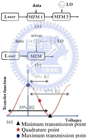
Figure 2-3 (a) and (b) are two schemes of transmitter and (c) is duty cycle of subcarrier biased at different points in the transfer function. (LO: local oscillator)... 8
Figure 2-4 Optical microwave/mm-wave modulation scheme by using MZM ... 10
Figure 2-5 The model of communication channel in a RoF system. ... 11
Figure 2-6 The model of receiver in a ROF system. ... 12
Figure 2-7 The model of ROF system. ... 12
Figure 2-8 Conceptual diagram of the proposed system ... 14
Figure 2-9 Modified SSB modulation scheme... 15
Figure 2-10 Frequency quadrupling scheme... 16
Figure 2-10 Frequency quadrupling scheme... 18
Figure 3-1 Illustration of modified SSB ... 23
VI
Figure 3-3 Illustration of signal pre-coding ... 26
Figure 4-1 Frequency quadrupling scheme... 28
Figure 4-2 Block diagrams of OFDM transmitter (a) and receiver (b). ... 29
Figure 4-3 Experimental Setup. EDFA: Erbium Doped Fiber Amplifier, OBPF: Optical BandPass Filter, PC: Polarization Controller, SSMF: Standard Single Mode Fiber, PD: Photo Detector. ... 31
Figure 4-4 OPR ... 33
Figure 4-5 OPR Constellations, (a) OPR=-1 (b) OPR=6 (c) OPR=9 ... 34
Figure 4-6 OSA ... 36
Figure 4-7 ESA ... 37
Figure 4-8 BER curves... 38
Figure 4-9 BER constellations with input power -8dBm ... 38
Figure 4-10 OPR ... 40
Figure 4-11 OPR Constellations, (a) OPR=0 (b) OPR=5 (c) OPR=10 ... 41
Figure 4-12 OSA ... 43
Figure 4-13 ESA ... 44
Figure 4-14 EVM curves ... 45
Figure 4-15 BER constellations with input power -8dBm... 45
Figure 4-16 Experimental Setup. EDFA: Erbium Doped Fiber Amplifier, OBPF: Optical BandPass Filter, PC: Polarization Controller, SSMF: Standard Single Mode Fiber, PD: Photo Detector. ... 46
Figure 4-17 three different kind pre-code constellations results... 48
Figure 5-1 (a) BER for 13.75-Gb/s QPSK-OFDM (b) EVM for 20.625-Gb/s 8QAM-OFDM ... 50
Figure 5-2 SNR for (a) 13.75-Gb/s QPSK-OFDM (b) 20.625-Gb/s 8QAM-OFDM ... 50
1
Chapter 1
Introduction
1.1 Review of Radio-over-fiber system
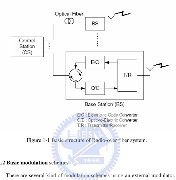
With rapidly increased for the next generation multi-media service , such as IEEE 802.15.3c WPAN, IEEE 802.16 WiMAX, and Wireless HD , the bandwidth requirement is also increased . Hence, to develop higher frequency microwave, even millimeter-wave is an important issue in the future. Traditionally, wireless system needs lots of Base station to deliver millimeter-wave signal, which would significant increase the cost . Now , another solution has been found , which is Radio-over-Fiber (RoF) system . RoF system is composed of central station (CS) , base station (BS) , as shown in Fig. 1-1. In RoF system, CS handles coding , up-conversion , and modulation, so BS just have to do the optic-to-electric or electric-to-optic conversion , which can reduce the complexity and cost of BS. CS and BS is connected by fiber. Fiber transmission medium is one of the best solutions because there are wider bandwidth and much less power loss in fiber. Therefore, RoF systems are attracted and more interesting for potential use in the future. RoF technology is a promising solution to provide multi-gigabits/sec service because of using millimeter wave band, and it has wide converge and mobility. The combination of orthogonal frequency-division multiplexing (OFDM) and radio-over-fiber (ROF) systems (OFDM-ROF) is considerable attention for future gigabit broadband wireless communication [1-5].
2
Figure 1-1 Basic structure of Radio-over fiber system.
1.2 Basic modulation schemes
There are several kind of modulation schemes using an external modulator, such as double-sideband (DSB), single-sideband (SSB), and double-sideband with optical carrier suppression (DSBCS) modulation, and these schemes have already been demonstrated on many publications [6-9]. Each modulation scheme has its own advantage and disadvantage, respectively. DSB is the most compact system, but it suffers inferior sensitivities due to limited optical modulation index (OMI), and fading issue because of fiber dispersion. SSB can overcome fading, but it suffers inferior sensitivities as well. Among these modulation schemes, DSBCS modulation has been demonstrated to be effective in the millimeter-wave range with excellent spectral efficiency, a low bandwidth requirement for electrical components, and superior receiver
3
sensitivity following transmission over a long distance [10-12]. Despite all these advantages, DSBCS schemes can only support on-off keying (OOK) format, but cannot transmit vector modulation formats, such as phase shift keying (PSK), quadrature amplitude modulation (QAM), or OFDM signals, which are of utmost importance for wireless applications.
This study proposes a modified single sideband (SSB) modulation scheme with frequency sextupling using two dual-parallel MZM, with frequency sextupling. A frequency multiplication scheme is employed to reduce the requirement of bandwidth of electronic components, which is an important issue at millimeter-wave RoF systems. Benchmarked against the OOK format, the 13.75-Gb/s QPSK-OFDM and 20.625-Gb/s 8-QAM-OFDM format has the higher spectral efficiency.
1.3 Motivation
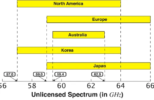
Recently, several countries have already released the unlicensed spectrum about 7GHz near the 60GHz band [13], as shown in Fig. 1-2 . However, the coverage of the 60-GHz wireless signals is limited by the high path and atmospheric losses , as shown in Fig. 1-3. To extend the signal coverage, radio-over-fiber (RoF) techniques become a promising solution for broad band wireless access networks. So in this work, we propose a new RoF system which has high spectral efficiency and satisfy the 60GHz applications. Additionally, we demonstrate that double sideband with carrier suppress (DSBCS) modulation scheme can also transmit vector signal by signal pre-coding.
4
Figure 1-2 Unlicensed Spectrum.
Figure 1-3 Atmospheric absorption of millimeter-wave signal .
5
Chapter 2
The Concept of New Optical Modulation System
2.1 Preface
Optical communication system is composed of optical transmitter, communication channel and optical receiver. In this chapter, we will do an introduction about how these three parts work, and what is the external
Mach-Zehnder Modulator (MZM), and how MZM construct a
Radio-over-Fiber (RoF) system. In the end, we will propose a new model of the RoF system.
2.2 Mach-Zehnder Modulator (MZM)
There are two ways to generate optical signal, which are direct modulation and external modulation. With the bandwidth requirement increase, it’s difficult to use direct modulation since the frequency chirp imposed on signal becomes large enough. Hence, most RoF systems are using external modulation with
phase modulator (PM) or Mach-Zehnder modulator (MZM) or
Electro-Absorption Modulator (EAM). The most commonly used MZM are based on LiNbO3 (lithium niobate) technology. According to the applied electric field, there are two types of LiNbO3 device : x-cut and z-cut. According to number of electrode, there are two types of LiNbO3 device:
dual-drive Mach-Zehnder modulator (DD-MZM) and single-drive
6
Figure 2-1 Most common electrode configurations for (a) non-buffered x-cut, (b)buffered x-cut, (c) buffered single-drive z-cut, and (d) buffered dual drive z-cut. [14]
7 2.3 Dual parallel Mach-Zehnder Modulator
By integrated technology, there is another kind of modulator called “dual parallel Mach-Zehnder Modulator”. Dual parallel Mach-Zehnder Modulator is composed of two MZM and one phase modulator, as shown in Fig. 2-2.This modulator is the most important component in the RoF system we proposed.
Figure 2-2 dual parallel Mach-Zehnder modulator configuration [15]
2.4 The architecture of ROF system 2.4.1 Optical transmitter
In RoF system, optical transmitter includes optical source, optical modulator, RF signal, electrical mixer, electrical amplifier, etc.. Presently, most RoF systems are using laser as light source. The advantages of laser are compact size, high efficiency, good reliability small emissive area compatible with fiber core dimensions, and possibility of direct modulation at relatively high frequency. The modulator is used for converting electrical signal into optical form. Because the external integrated modulator was composed of MZMs, we select MZM as modulator to build the architecture of optical transmitter.
8
scheme is used two MZM. First MZM generates optical carrier which carried the data. The output optical signal is BB signal. The other MZM generates optical subcarrier which carried the BB signal and then output the RF signal, as shown in Fig. 2-3 (a). The other scheme is used a mixer to get up-converted electrical signal and then send it into a MZM to generate the optical signal, as shown in Fig. 2-3 (b). Fig. 2-3 (c) shows the duty cycle of subcarrier biased at different points in the transfer function.
Maximum transmission point Minimum transmission point Quadrature point
Figure 2-3 (a) and (b) are two schemes of transmitter and (c) is duty cycle of subcarrier biased at different points in the transfer function. (LO: local
9
2.4.2 Optical signal generations based on LiNbO3 MZM
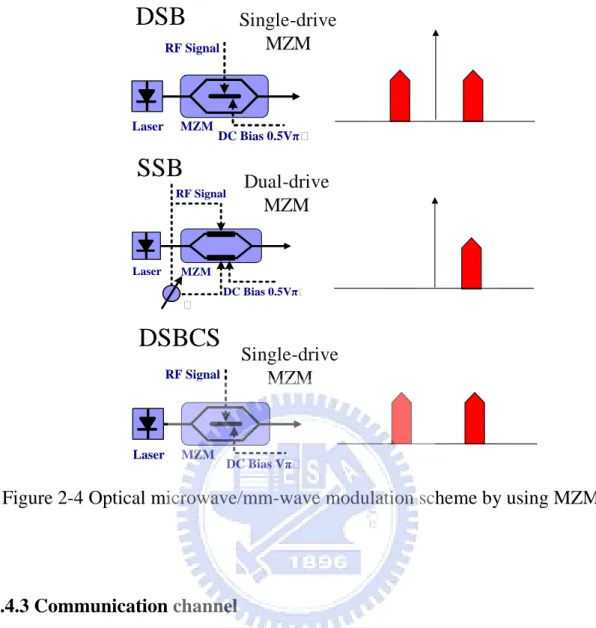
The microwave and mm-wave generations are key techniques in RoF systems. The optical mm-waves using external MZM based on double-sideband (DSB), single-sideband (SSB), and double-sideband with optical carrier suppression (DSBCS) modulation schemes have been demonstrated, as shown in Fig. 2-4. Generated optical signal by setting the bias voltage of MZM at quadrature point, the DSB modulation experiences performance fading problems due to fiber dispersion, resulting in degradation of the receiver sensitivity. When an optical signal is modulated by an electrical RF signal, fiber chromatic dispersion causes the detected RF signal power to have a periodic fading characteristic. The DSB signals can be transmitted over several kilo-meters. Therefore, the SSB modulation scheme is proposed to overcome fiber dispersion effect. The SSB signal is generated when a phase difference of π/2 is applied between the two RF electrodes of the DD-MZM biased at quadrature point. Although the SSB modulation can reduce the impairment of fiber dispersion, it suffers worse receiver sensitivity due to limited optical modulation index (OMI). The DSBCS modulation is demonstrated optical mm-wave generation using DSBCS modulation. It has no performance fading problem and it also provides the best receiver sensitivity because the OMI is always equal to one. The other advantage is that the bandwidth requirement of the transmitter components is less than DSB and SSB modulation. However, the drawback of the DSBCS modulation is that it can’t support vector signals, such as phase shift keying (PSK), quadrature amplitude modulation (QAM), or OFDM signals, which are of utmost importance in wireless applications.
10
Figure 2-4 Optical microwave/mm-wave modulation scheme by using MZM
2.4.3 Communication channel
Communication channel concludes fiber, optical amplifier, etc.. Presently, most RoF systems are using single-mode fiber (SMF) or dispersion compensated fiber (DCF) as the transmission medium. When the optical signal transmits in optical fiber, dispersion will be happened. DCF is use to compensate dispersion. The transmission distance of any fiber-optic communication system is eventually limited by fiber losses. For long-haul systems, the loss limitation has traditionally been overcome using regenerator witch the optical signal is first converted into an electric current and then regenerated using a transmitter. Such regenerators become quite complex and expensive for WDM lightwave systems. An alternative approach to loss
DSB
SSB
Dual-drive MZM DC Bias 0.5Vπ MZM Laser RF Signal DC Bias 0.5Vπ MZM Laser RF Signal DC Bias Vπ MZM Laser RF SignalDSBCS
Single-drive MZM Single-drive MZM11
management makes use of optical amplifiers, which amplify the optical signal directly without requiring its conversion to the electric domain [16]. Presently, most RoF systems are using erbium-doped fiber amplifier (EDFA). An optical band-pass filter (OBPF) is necessary to filter out the ASE noise. The model of communication channel is shown in Fig. 2-5.
Figure 2-5 The model of communication channel in a RoF system.
2.4.4 Demodulation of optical millimeter-wave signal
Optical receiver concludes photo-detector (PD), demodulator, etc.. PD usually consists of the photo diode and the trans-impedance amplifier (TIA). In the microwave or the mm-wave system, the PIN diode is usually used because it has lower transit time. The function of TIA is to convert photo-current to output voltage.
The BB and RF signals are identical after square-law photo detection. We can get RF signal by using a mixer to drop down RF signal to baseband then filtered by low-pass filter (LPF).
After getting down-converted signal, it will be sent into a signal tester to test the quality, just like bit-error-rate (BER) tester or oscilloscope, as shown in Fig. 2-6.
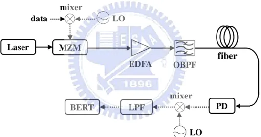
Combining the transmitter with communication channel and receiver, that is the model of ROF system, as shown in Fig. 2-7. We select the scheme of Fig. 2-5 (b) to become the transmitter in the model of ROF system.
12
Figure 2-6 The model of receiver in a ROF system.
Figure 2-7 The model of ROF system.
Laser MZM data mixer LO OBPF EDFA fiber PD LPF mixer LO BERT
13
2.5 The new proposed model of optical modulation system 2.5.1 Conceptual diagram of the proposed system
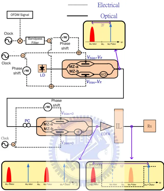
In previous section, we introduce three kind of modulation schemes to generate optical RF signal. In this work, a modified single sideband (SSB) modulation scheme with frequency sextupling using two dual-parallel MZM is proposed. Fig. 2-8 shows the conceptual diagram of the proposed system. The transmitter of the proposed system would be easier to understand if we separate it to two parts. So next, we will introduce these two parts in details.
14 MZ-a MZ-b π MZ-a MZ-b π/2 LD Electrical Optical Phase shift +90∘ Phase shift +90∘ Clock x x Clock OFDM Signal Bandpass Filter Vbias=0 Vbias=0 Clock PC
IL
Rx Vbias=Vπ Vbias=Vπ EDFA ω ωo ωo-ωRF ωo+ωRF ω ωo ωo-ωRF ωo+ωRF ωo-3ωRF ωo+3ωRF 2F ω ωo ωo-ωRF ωo+ωRF ωo-3ωRF ωo+3ωRF 6F Phase shift +90∘Figure 2-8 Conceptual diagram of the proposed system
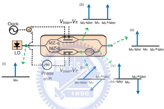
2.5.2 Modified SSB modulation scheme
The first part of the transmitter in the proposed system is modified single-sideband (SSB) modulation, as shown in Fig. 2-9. For simplicity, the figure shows only one RF signal. Since MZ-a and MZ-b are biased at null point, the output spectrum are both double-sideband with optical carrier suppression (DSBCS). The only difference between MZ-a and MA-b is phase term.
15
at -ωRF term. After that, a π/2 phase shift is introduced at lower arm, and then
combines the two arms. Finally, a new optical carrier is obtained at ωo-ωRF
term. OFDM signal can be obtained at ωo+ωRF term in the same way.
Modified SSB modulation is important to the proposed system since it provide not only a direct-detection OFDM modulation scheme but also frequency doubling result.
MZ-a MZ-b π/2 LD Phase shift +90∘ Clock x Vbias=Vπ Vbias=Vπ ωo ω o ωo-ωRF ωo+ωRF ωo ωo-ωRF ωo+ωRF ωo ωo-ωRF ωo+ωRF ωo ωo-ωRF ωo+ωRF (i) (ii) (iv) (iii) (v)
Figure 2-9 Modified SSB modulation scheme
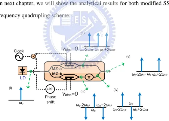
2.5.3 Frequency quadrupling scheme
This part of the transmitter in the proposed system is frequency quadrupling, as shown in Fig. 2-10. For simplicity, the figure shows only one optical input. Since MZ-a and MZ-b are biased at full point, the output spectrum are both double-sideband (DSB). The only difference between MZ-a
and MA-b is phase term. Compare to MZ-a, MZ-b has +π phase shift at +2ωRF
16
lower arm, and then combines the two arms. Finally, frequency quadrupling result is obtained.
Frequency quadrupling technique is needed for this system because the entire electrical component with frequency above 30GHz would be extremely expensive, which would significant increase the cost of transmitter. With frequency quadrupling technique, this is no longer a problem in the proposed system.
When combine the modified SSB modulation scheme and frequency modulation scheme, the sextupling direct-detection OFDM RoF system is appeared.
In next chapter, we will show the analytical results for both modified SSB and frequency quadrupling scheme.
MZ-a MZ-b π LD Phase shift +90∘ Clock x Vbias=0 Vbias=0 ωo ωo ωo-2ωRF ωo+2ωRF (i) (ii) (iv) (iii) (v) ωo ωo-2ωRF ωo+2ωRF ωo ωo-2ωRF ωo+2ωRF ωo ωo-2ωRF ωo+2ωRF
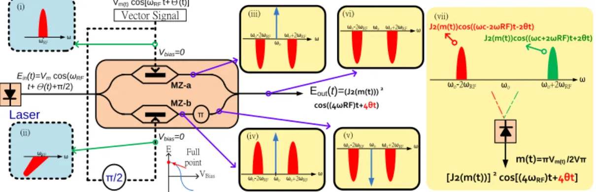
17 2.5.4 Signal Pre-coding
Traditionally, double sideband with carrier suppress (DSBCS) modulation scheme cannot transmit vector signal since the phase term of signal would distort. Frequency quadrupling is kind of like a modified DSBCS, so it cannot transmit vector signal as well. After calculation, we find out how distortion occurs, and the rule of this distortion [17]. In another words, we can still put vector signal to this system by some mathematical tricks. The calculation details will be shown at next chapter.
18 ω ωo ωo-2ωRF ωo+2ωRF DC Bias MZ-a MZ-b Vbias=0 Ein(t)=Vm cos(ωRF t+Θ(t)+π/2) Vbias=0 π π/2 Laser Eout(t)=(J2(m(t))) 2 cos((4ωRF)t+4θt) Full point E VBias ω ωo ωo-2ωRF ωo+2ωRF ω ωo ωo-2ωRF ωo+2ωRF ωo ωo+2ωRF ωo-2ωRF ω J2(m(t))cos((ωc+2ωRF)t+2θt) J2(m(t))cos((ωc-2ωRF)t-2θt) [J2(m(t))] 2 cos[(4ωRF)t+4θt] ω ωRF ω ωRF Vector Signal (i) (ii) (iii) (iv) (vi) ω ωo ωo-2ωRF ωo+2ωRF (v) (vii) Vm(t) cos[ωRF t+Θ(t)] m(t)=πVm(t) /2Vπ
Figure 2-11 Frequency quadrupling scheme
Chapter 3
Theoretical calculations of the proposed system
3.1 Preface
In this chapter, we will show the analytical results for both modified SSB scheme and frequency quadrupling scheme. The discussion will start from what is Bessel expansion, and how MZM works, and then show the calculation details.
19 3.2 Bessel expansion
Before we discuss about the theoretical calculation, first we have to know the following Bessel expansions. Bessel function is defined as
/2 /1
, n n n x t t J x t g x t e
And if we take i te, we have
sin ix n n n J x t e
Use the identity Jn
x 1n Jn x , we have
1 2 2 1 1 1 2 2 2 2 2 sin 2 cos 2 i i i i i i i i J x e e e i J x e e e J x e J x J x J x e J x J x Therefore we will have
These four equations are really important and helpful of our calculations.
3.3 MZM output electrical field
Dual-parallel MZM is composed of three sub MZMs, so we will first introduce how MZM works. The output electrical field of MZM can be written as
cos cos out Eo ot E Where20 1 V V o
is frequency of light source, Vis the voltage to change MZM to
phase shift, and V1 is the input signal. We can write input signal as
1 0 ( ) cos( ) cos( ) cos( ) cos[ ] 2 bias m RF bias m RF bias m RF OUT V t V V w t V V w t V V V V V w t E E V bias
V is DC input and Vmcos(w tRF )is RF input. Then we set
0 0 0 0 0 0 2 2 cos( ) cos[ ]cos( ) 2 cos[ c cos[ cos( os( )]cos( ){cos( ) )] sin sin[ cos( )]}cos( )
b R ias m bias m RF OUT RF F RF V b V V m v V V w t E E w t V E b m w m w t m w t t w t E b b w t
This equation can be expanded by Bessel equations as below.
0 0 0 0 2 1 2 1 1 0 0 0 2 1 0 0 0 2 1 [ ( ) 2 ( 1) ( ) cos(2 )]cos [2 ( 1) ( ) cos[(2 1) ]] {cos( ) ( ) sin( ) cos( )} cos( ) ( ) cos( ) cos( ) ( 1) ( ) cos[ ] cos ( 2 ) ( ) ( 1) ( ) co n n RF n n out n n n n RF n R n F n n E E b w t b w t E b J m E b J m J m nw J m t J m n w t w nw t w t E b J m
0 2 1 1 0 0 2 1 0 1 0 ( 2 ) ( (2 1) s[ ] sin( ) ( 1) ( ) cos[ ] sin( ) ( 1) ( ) cos[ ] ) ( (2 1) ) n n n n n RF RF n RF w nw t w E b J m E b J m n w t w n w t
21
interesting result. This is the basic idea of modified SSB and frequency quadrupling.
3.4 Theoretical calculation of modified SSB
Configuration of the dual parallel MZM we used in our demonstration is
shown at figure 2.2. We bias MZ-a, which means the upper arm, atV, so the
output electrical field would be
0 2 1 0 1 2 1 0 1 2 ( 1) ( ) cos[( (2 1) ) ] ( 1) ( ) cos[( (2 1) ) ] n upper n RF n n n RF n E E J m w n w t J m w n w t b
MZ-b, the lower arm, is also biased at V, but RF signal has a
2
phase shift. Also, light source has a
2
phase shift which is induced by MZ-c. Then we can derive the lower arm output as
22
0 0 0 0 0 0 0 0 2 0 1 2 1 sin( ) cos[ ]sin( ) 2cos[ sin( )]sin( )
{cos( ) cos[ sin( )] sin sin[ sin( )]}sin( )
{cos( )[ ( ) 2 ( ) cos(2 )]sin( )
sin( )[2 ( ) sin[(2 1 bias m RF lower RF RF RF n RF n n V V w t E E w t V E b m w t w t E b m w t b m w t w t E b J m J m nw t w t b J m n
0 1 0 0 0 0 2 0 1 0 2 0 1 0 2 1 0 1 0 2 1 0 1 ) ]]sin( )} cos( ) ( ) sin( ) cos( ) ( ) sin[( 2 ) ] cos( ) ( ) sin[( 2 ) ] sin( ) ( ) cos[( (2 1) ) ] sin( ) ( ) cos[( (2 1) ) ] RF n n RF n n RF n n RF n n RF n w t w t E b J m w t E b J m w nw t E b J m w nw t E b J m w n w t E b J m w n w t
0 2 1 0 1 0 2 1 0 1 2 ( ) cos[( (2 1) ) ] ( ) cos[( (2 1) ) ] lower n RF n RF n n E b E J m w n w t E J m w n w t
Then combine the upper arm and lower arm electrical field, we can get the total output electrical field of dual parallel MZM.
0 2 1 0 0 0 1 2 1 0 1 0 2 1 0 1 0 2 1 0 1 0 1 0 3 ( 1) ( ) cos[( (2 1) ) ] ( 1) ( ) cos[( (2 1) ) ] 2 3 2 ( ) cos[( (2 1) ) ] ( ) cos[( (2 1) ) ] ( ) cos ( ) cos R n out n RF F R n n n RF n F RF n n RF n n E E J m w n w t J m w n w t J t J w w w t w E J m w n w t E J m w n w t E m E m
0
5 0 2 .. .. 5 . .. ( ) cos RF J w w t E m 23
The figure below shows what the spectrum looks like. We can use the same way to get another signal opposite, and then modified SSB is obtained.
W0+WRF W0-3WRF W0 W0+2WRF W0+4WRF W0+5WRF W0-2WRF W0-4WRF
Figure 3-1 Illustration of modified SSB
3.5 Theoretical calculation of frequency quadrupling
To get the frequency quadrupling, we first bias MZ-a, the upper arm, at 0. Which implies b=0. So output electrical field of upper arm is
0 0 0 0 2 0 1 0 2 0 1 ( ) cos( ) ( 1) ( ) cos[( 2 ) ] ( 1) ( ) cos[( 2 ) ] upper n n RF n n n RF n E E J m w t E J m w nw t E J m w nw t
MZ-b, the lower arm, is also biased at 0, but RF signal has a 2
phase shift,
and light source has a phase shift which is induced by MZ-c. Then we can
24
0 0 0 0 0 0 0 0 2 0 1 2 1 sin( ) cos[ ]cos( ) 2cos[ sin( )]cos( )
{cos( ) cos[ sin( )] sin sin[ sin( )]}cos( )
{cos( )[ ( ) 2 ( ) cos(2 )]cos( )
sin( )[2 ( ) sin[( bias m RF lower RF RF RF n RF n n V V w t E E w t V E b m w t w t E b m w t b m w t w t E b J m J m nw t w t b J m
0 1 0 0 0 0 2 0 1 0 2 0 1 0 2 1 0 1 0 2 1 0 2 1) ]]cos( )} cos( ) ( ) cos( ) cos( ) ( ) cos[( 2 ) ] cos( ) ( ) cos[( 2 ) ] sin( ) ( ) sin[( (2 1) ) ] sin( ) ( ) sin[( (2 1) ) ] RF n n RF n n RF n n RF n n RF n n w t w t E b J m w t E b J m w nw t E b J m w nw t E b J m w n w t E b J m w n w t
1 0 0 0 0 2 0 1 0 2 0 1 0 ( ) cos( ) ( ) cos[( 2 ) ] ( ) cos[( 2 ) ] lower RF n n RF n n E b E J m w t E J m w nw t E J m w nw t
Then combine the upper arm and lower arm electrical field, we can get the total output electrical field of dual parallel MZM.
0 2 0 1 0 2 0 1 0 2 0 1 0 0 0 0 2 0 1 0 2 0 6 0 10 2 2 2 6 ( 1) ( ) cos[( 2 ) ] ( 1) ( ) cos[( 2 ) ] ( ) cos[( 2 ) ] ( ) cos[( 2 ) ] ( ) cos[( ) ] ( ) cos[( ) ] ( ) cos[ 2 ( out RF R n RF n n n RF n n RF n n R F F n n E E J m w nw t E J m w nw t E J m w nw t E J m w nw t E J m t E w w w w J m t E J m w
10 ) ] ... RF w t 25
The figure below shows how the spectrum looks like.
W0+2WRF W0-6WRF W0 W0+2WRF W0+4WRF W0-2WRF W0-4WRF W0+2WRF W0+6WRF
Figure 3-2 Illustration of frequency quadrupling
3.6 Theoretical calculation of signal pre-coding
Refer to the analytical result of frequency quadrupling, that is
0 2 0 0 6 0 0 10 0 2 2 6 2 10 ( ) cos[( 2 ) ] ( ) cos[( ) ] ( ) cos[( ) ] ... out RF RF RF E E J m w w t E J m w w t E J m w w t If we replace wRFbywRF ,
0 2 0 0 6 0 0 10 0 2 2 6 2 10 ( ) cos[( 2 ) ] ( ) cos[( ) ] ( ) cos[( ) ] ... out RF RF RF E w w w E J m w t E J m w t E J m w t And ignore high order term,2 2
( ) { [ ( )] cos[( 2 ) 2 ( )] [ ( )] cos[( 2 ) 2 ( )]}
out o o RF o RF
E t E J m t t t J m t t t
After PD square law, we get
2 4 2 4 1 ( ) [ ( )] co [ ( ] 2 s 4 ) RF RF i t R J m t t t
From this equation, we find out what the phase distortion in frequency quadrupling is. So if we choose the proper position in 16PSK at transmitter
26
node, then a QPSK constellation would occur at receiver node, as shown in Fig. 3-3.
27
Chapter 4
Combination of Orthogonal Frequency-Division and
Radio-over-Fiber Systems
4.1 Preface
In chapter 2, the whole idea of the proposed system is introduced. In this chapter, we will first talk about what is OFDM, and then demonstrate the proposed system, and show the experimental results.
4.2 Orthogonal frequency division multiplexing
Basically, orthogonal frequency division multiplexing (OFDM) means using a large number of parallel narrow-band subcarriers instead of a single wide-band carrier to transport information, as shown in Fig. 3-1. There would be lots of significant advantages since the relative low bandwidth of each subcarrier, and of course, some trade off.
The most important advantage of OFDM is the bandwidth efficiency. Performance of single carrier system would be restricted by channel response, which means the bandwidth cannot achieve too high, and data format as well. But in OFDM system, it’s easy to overcome the channel response by using a one tap equalizer since it has only low bandwidth subcarriers.
Dispersion tolerance is also an advantage of OFDM. When a broad band light signal transmits in fiber, transmission distance is restricted by dispersion coefficient, which is typically 16ps/km-nm in single mode fiber. But in OFDM system, again, since it has only low bandwidth subcarriers, dispersion is no longer an issue.
28
the large computational amount. OFDM is impossible to realize because the computational amount is too large, until mathematician invent the fast Fourier transform (FFT) to reduce the computational amount. But still, computational amount is an issue of OFDM.
Another main disadvantage of OFDM is the peak-to-average-ratio (PAPR). When all the subcarrier of OFDM is in the same phase, system may appear a peak power that is much higher than the average power. This may induce a large noise to signal. There are some algorithms to reduce the impact of PAPR, but they still have their own tradeoff. However, PAPR is a weakness of OFDM system.
OFDM has its own advantages and disadvantages. And as we mentioned at chapter 1-3, bandwidth efficiency would be the top priority of the proposed system, so OFDM is utilize in the proposed system. The detail of OFDM signal generation is illustrated in Fig. 3-2.
Single high data rate subcarrier
Frequency
Replaced by multiple lower data rate subcarrier
Figure 4-1 Frequency quadrupling scheme
Serial to parallel Parallel to serial conversion Cyclic prefix insertion
Offline DSP program AWG
DAC QAM
modulation IFFT
29
ADC FFT decoderQAM to serialParallel
Offline DSP program Digital Scope Channel estimation and one-tap equalization Serial to parallel conversion Timing Synchro-nization (b)
Figure 4-2 Block diagrams of OFDM transmitter (a) and receiver (b).
4.3 Experimental setup of Optical direct-detection for RoF link
Figure 4-3 shows the experimental setup of the proposed system. A modified SSB signal with frequency doubling is generated using a dual-parallel MZM. Then, the modified SSB signal is sent into the proposed colorless optical up-conversion system with frequency quadrupling. To select the desired optical sidebands and obtain the modified SSB signal with frequency sextupling, an optical interleaver is utilized. Based on the modified SSB modulation scheme, there is no dispersion-induced performance fading, and high spectral efficiency orthogonal frequency-division multiplexing (OFDM) modulation format is experimentally demonstrated. Because the optical powers of the OFDM modulated and the unmodulated optical sidebands can be freely adjusted by controlling the amplitude of the driving signals, the receiver performance can be optimized by adjusting the optical power ratio (OPR) between the OFDM modulated and the unmodulated optical sidebands. Because of the colorless
up-conversion system, wavelength-division-multiplexing (WDM)
up-conversion sharing only one optical up-conversion system can be achieved. Most importantly, only 10-GHz components and equipments which can provide better performance and lower costs compared with higher frequency components are required in this proposed system.
30
There are two kinds of data format has been demonstrated in this work, including 13.75-Gb/s QPSK-OFDM, 20.625-Gb/s 8QAM-OFDM. Detail will be shown in the following section, respectively.
31 MZ-a MZ-b π MZ-a MZ-b π/2 DFB Laser
Electrical
Optical
Phase shift +90∘ Phase shift +90∘ 10GHz x AWGVbias=0
Vbias=0
10GHzPC
Vbias=V
πVbias=V
π EDFA Phase shift +90∘ In te rl e a v e r SSMF PD Bandpass Filter 55GHz Scope 60GHz (1) (2) EDFA OBPF EDFA OBPF (a) (b) (c) (d) (e) (3)Figure 4-3 Experimental Setup. EDFA: Erbium Doped Fiber Amplifier, OBPF: Optical BandPass Filter, PC: Polarization Controller, SSMF: Standard Single Mode Fiber, PD: Photo Detector.
32
4.4 Experimental results of 13.75-Gb/s QPSK-OFDM 4.4.1 The optimal optical power ratio condition
In the beginning, we try to transmit data-rate 13.75-Gb/s, total bandwidth 6.875GHz QPSK-OFDM signal. First, we have to find optimal optical power ratio first. Figure 3-16 shows the experimental results of the OPR optimization. The OPR is defined as unmodulated sideband optical power to OFDM modulated sideband optical power ratio. When the OPR equals to 6 dB, the receiver has the best performance. The constellations of different OPR are shown in figure 3-17.
33 (a) (b) (c) -2 0 2 4 6 8 10 12 11 10 9 8 7 6 -l o g (BER ) OPR Figure 4-4 OPR
34
Figure 4-5 OPR Constellations, (a) OPR=-1 (b) OPR=6 (c) OPR=9
4.4.2 OFDM details
The up-converted OFDM signal is generated with 20-GHz DAC sampling rate, 256 FFT size, 88 subcarriers, each subcarrier has 78.125-MHz bandwidth, total bandwidth 6.875-GHz, and data-rate 13.75-Gb/s.
35 4.4.3 Transmission results
Figure 4-6 shows optical spectrum in this demonstration. Mark (a)~(e) relates to figure 4-3. (a) is the output spectrum at first stage, which is the modified SSB signal. (b) is the spectrum after EDFA and optical bandpass filter. Optical bandpass filter here is used to filter out amplified spontaneous emission (ASE) from EDFA. (c) is the output spectrum at second stage, which is the modified SSB signal after frequency quadrupling. (d) is the spectrum after interleaver. (e1) is the spectrum without transmission, (e2) is 50km transmission, (e3) is 100km transmission.
Figure 4-7 shows electrical spectrum in this demonstration. Mark (1)~(3) relates to figure 4-3. (1) is the output spectrum of AWG. Since signal in this figure is still at base band, the total bandwidth is only 3.5-GHz. (2) is the spectrum after up-convert to 10-GHz. (3-1) is the spectrum of received signal after down-convert to 5-GHz without transmission. (3-2) is 50km transmission. (3-3) is 100km transmission.
Figure 4-8 shows the estimated bit error rate (BER) curves of the 60-GHz 13.75-Gb/s QPSK-OFDM signal. After the transmission of 50km SSMF, receiver power penalty is observed about 0.5dB. And after the transmission of 100km SSMF, receiver power penalty is observed about 1dB. The constellations of the QPSK-OFDM signals are shown in figure 4-9.
36 (a) (b) (c) (d) (e1) (e2) (e3) 1547.5 1547.6 1547.7 1547.8 1547.9 -80 -70 -60 -50 -40 -30 -20 Le vel (dBm ) WaveLength(nm) 1547.5 1547.6 1547.7 1547.8 1547.9 -50 -40 -30 -20 -10 0 Le vel (dBm ) WaveLength(nm) 1547.2 1547.4 1547.6 1547.8 1548.0 1548.2 -80 -70 -60 -50 -40 -30 -20 Le vel (dBm ) WaveLength(nm) 1547.2 1547.4 1547.6 1547.8 1548.0 1548.2 -80 -70 -60 -50 -40 -30 -20 Le vel (dBm ) WaveLength(nm) 1547.2 1547.4 1547.6 1547.8 1548.0 1548.2 -40 -30 -20 -10 0 10 Le vel (dBm ) WaveLength(nm) 1547.2 1547.4 1547.6 1547.8 1548.0 1548.2 -40 -30 -20 -10 0 10 L e ve l( d B m ) W a ve Len gth (n m) 1547.2 1547.4 1547.6 1547.8 1548.0 1548.2 -40 -30 -20 -10 0 10 L e ve l( d B m ) W a ve Len gth (n m) Figure 4-6 OSA
37 (1) (2) (3-1) (3-2) (3-3) 0 1 2 3 4 5 6 -100 -90 -80 -70 -60 -50 -40 L e ve l( d B m ) Freq uen cy (GH z) 6 8 10 12 14 -90 -80 -70 -60 -50 -40 -30 -20 L e ve l( d B m ) Freq uen cy (GH z) 0 2 4 6 8 10 -90 -80 -70 -60 -50 -40 -30 -20 -10 L e ve l( d B m ) Freq uen cy (GH z) 0 2 4 6 8 10 -90 -80 -70 -60 -50 -40 -30 -20 -10 L e ve l( d B m ) Freq uen cy (GH z) 0 2 4 6 8 10 -90 -80 -70 -60 -50 -40 -30 -20 -10 L e ve l( d B m ) Freq uen cy (GH z) Figure 4-7 ESA
38 -13 -12 -11 -10 -9 -8 -7 10 9 8 7 6 5 4 3 2 BTB 50km 100km -l o g (BER ) Level(dBm)
Figure 4-8 BER curves
39
4.5 Experimental results of 20.625-Gb/s 8QAM-OFDM 4.5.1 The optimal optical power ratio condition
After finishing data-rate 13.75-Gb/s demonstration, we try to increase data-rate to 20.625-Gb/s by changing data format from total bandwidth 6.875GHz QPSK-OFDM to total bandwidth 6.875GHz 8QAM-OFDM. Just like what we do before, we have to find optimal optical power ratio first. Figure 4-10 shows the experimental results of the OPR optimization. The OPR is defined as unmodulated sideband optical power to OFDM modulated sideband optical power ratio. When the OPR equals to 5 dB, the receiver has the best performance. The constellations of different OPR are shown in figure 4-11.
40 (a) (b) (c) 0 2 4 6 8 10 6 7 8 9 10 11 E V M( %) OPR Figure 4-10 OPR
41
Figure 4-11 OPR Constellations, (a) OPR=0 (b) OPR=5 (c) OPR=10
4.5.2 OFDM details
The up-converted OFDM signal is generated with 20-GHz DAC sampling rate, 256 FFT size, 88 subcarriers, each subcarrier has 78.125-MHz bandwidth, total bandwidth 6.875-GHz, and data-rate 20.625-Gb/s.
42 4.5.3 Transmission results
Figure 4-12 shows optical spectrum in this demonstration. Mark (a)~(e) relates to figure 4-3. (a) is the output spectrum at first stage, which is the modified SSB signal. (b) is the spectrum after EDFA and optical bandpass filter. Optical bandpass filter here is used to filter out amplified spontaneous emission (ASE) from EDFA. (c) is the output spectrum at second stage, which is the modified SSB signal after frequency quadrupling. (d) is the spectrum after interleaver. (e1) is the spectrum without transmission, (e2) is 50km transmission, (e3) is 100km transmission.
Figure 4-13 shows electrical spectrum in this demonstration. Mark (1)~(3) relates to figure 4-3. (1) is the output spectrum of AWG. Since signal in this figure is still at base band, the total bandwidth is only 3.5-GHz. (2) is the spectrum after up-convert to 10-GHz. (3-1) is the spectrum of received signal after down-convert to 5-GHz without transmission. (3-2) is 50km transmission. (3-3) is 100km transmission.
Figure 4-14 shows the estimated error vector magnitude (EVM) curves of the 60-GHz 20.625-Gb/s QPSK-OFDM signal. Definition of EVM is
[18], where Perroris the RMS power of
the error vector, and Preference is the RMS power of ideal transmitted signal.
After the transmission of 50km SSMF, no significant receiver power penalty is observed. But after the transmission of 100km SSMF, receiver power penalty is observed about 1dB. The constellations of the QPSK-OFDM signals are shown in figure 4-15.
43 (a) (b) (c) (d) (e1) (e2) (e3) 1547.5 1547.6 1547.7 1547.8 1547.9 -80 -70 -60 -50 -40 -30 -20 Le ve l( dB m) WaveLength(nm) 1547.5 1547.6 1547.7 1547.8 1547.9 -50 -40 -30 -20 -10 0 L e ve l(dB m) WaveLength(nm) 1547.2 1547.4 1547.6 1547.8 1548.0 1548.2 -80 -70 -60 -50 -40 -30 -20 L e ve l(dB m) WaveLength(nm) 1547.2 1547.4 1547.6 1547.8 1548.0 1548.2 -80 -70 -60 -50 -40 -30 -20 L e ve l(dB m) WaveLength(nm) 1547.2 1547.4 1547.6 1547.8 1548.0 1548.2 -40 -30 -20 -10 0 10 L e ve l(dB m) WaveLength(nm) 1547.2 1547.4 1547.6 1547.8 1548.0 1548.2 -40 -30 -20 -10 0 10 L e ve l(dB m) WaveLength(nm) 1547.2 1547.4 1547.6 1547.8 1548.0 1548.2 -40 -30 -20 -10 0 10 L e ve l(dB m) WaveLength(nm) Figure 4-12 OSA
44 (1) (2) (3-1) (3-2) (3-3) 0 1 2 3 4 5 6 -100 -90 -80 -70 -60 -50 -40 Le ve l( dB m) Frequency(GHz) 6 8 10 12 14 -90 -80 -70 -60 -50 -40 -30 -20 L e ve l(dB m) Frequency(GHz) 0 2 4 6 8 10 -90 -80 -70 -60 -50 -40 -30 -20 -10 L e ve l(dB m) Frequency(GHz) 0 2 4 6 8 10 -90 -80 -70 -60 -50 -40 -30 -20 -10 L e ve l(dB m) Frequency(GHz) 0 2 4 6 8 10 -90 -80 -70 -60 -50 -40 -30 -20 -10 L e ve l(dB m) Frequency(GHz) Figure 4-13 ESA
45 -15 -14 -13 -12 -11 -10 -9 -8 -7 -6 -5 10 15 20 25 30 BTB 50km 100km EVM(% ) Power(dBm)
Figure 4-14 EVM curves
46 4.6 Experimental setup of signal pre-coding
Figure 4-16 shows the experimental setup of signal pre-code system. The symbol-rate 312.5-MSym/s pre-coded RF signal with center frequency at 2.5 GHz is generated by a Tektronix® AWG7102 arbitrary waveform generator (AWG) using a Matlab® program. After the AWG, the RF signal is up-converted to 15 GHz and then send into the integrated MZM. The generated optical signal is amplified using an erbium-doped fiber amplifier and then pass through an optical band-pass filter to remove the ASE noise. Following 50 km of SMF, the received RF signal is down-converted to 5 GHz and captures by digital real time scope (Tektronix DPO 71254). An offline program using Matlab is used to demodulate the QPSK RF signal.
Three different kind pre-code constellations are shown in figure 4-16. Performance of them will be shown in next section.
MZ-a MZ-b Vbias=0 Ein(t) Vbias=0 π π/2 Laser Eout(t) Pre-code 312.5 Msymbol/s QPSK at 2.5 GHz BW=0.4nm OBPF Optical Attenuator EDFA 25/50km SSMF Amp. Real Time Oscilloscope BPF 55GHz O/E 15 GHz BPF (i) 0-1-2-3 (ii) 0-5-10-15 (iii) 0-1-10-11 EDFA 12.5GHz
Figure 4-16 Experimental Setup. EDFA: Erbium Doped Fiber Amplifier, OBPF: Optical BandPass Filter, PC: Polarization Controller, SSMF: Standard Single Mode Fiber, PD: Photo Detector.
47
4.7 Experimental results of 312.5-Msym/s pre-code QPSK
0-1-2-3, 0-1-10-11, 0-5-10-15 three different kind pre-code constellations results are shown in figure 4-17. Obviously, performance of 0-1-2-3 is better than the other two. The reason supposed to be the different trace they need. To 0-1-2-3 pre-code, any transition angle is less than 2π. But to 0-1-10-11 and 0-5-10-15 pre-code, transition angle may be more than 2π, which means the trace of these two format is much longer than 0-1-2-3 format, so the constellation may not as precisely as 0-1-2-3 format.
48
49
Chapter 5
Discussion and Simulation
5.1 Preface
In chapter 4 all the experimental results are shown. But there is something strange about the penalty after transmission. In this chapter, we will discuss about that by doing some simulations.
5.2 Discussion
OFDM means you separate one wide bandwidth carrier to several narrow bandwidth subcarriers. In our demonstration, each subcarrier has only 78.125MHz bandwidth and modulated light signal transmit in standard single mode fiber (SSMF). Dispersion coefficient of SSMF is 16ps/km-nm. After 100km transmission, delay cause by dispersion is about 2.01ps, which is only 0.16% of OFDM symbol time and it would be compensated by cyclic prefix (CP) easily. So dispersion is definitely not the reason of the penalty. To find out how this penalty comes, we will do some simulations below using the
commercial software, VPI WDM-TransmissionMaker© 7.5.
5.3 Simulation
After trying all the possibilities, we finally find out the crucial reason of how the penalty comes, linewidth of laser. In our demonstration, DFB laser is used as the light source. Typically, linewidth of DFB laser is about 1~3MHz, and this may not be an issue generally. But when 60GHz signal is transmitting 100km in SSMF, trouble is coming. As shown in figure 5-1, laser linewidth may seriously interfere with signal after transmission. 13.75-Gb/s QPSK-OFDM and 20.625-Gb/s 8QAM-OFDM are just the same. To compare these two kind data format, figure 5-2 shows the signal-to-noise-ratio (SNR).
50
From this simulation result, we can clearly see that the only way to improve performance of this system is using another laser such as tunable laser (TL) which linewidth is much narrower than DFB laser.
(a) (b) 1k 10k 100k 1M 10M 11 10 9 8 7 6 5 -Log(BER) linewidth (Hz) BTB 50km 100km 1k 10k 100k 1M 10M 7.5 8.0 8.5 9.0 9.5 10.0 10.5 11.0 11.5 12.0 12.5 13.0 13.5 14.0 14.5 15.0 EVM linewidth (Hz) BTB 50km 100km
Figure 5-1 (a) BER for 13.75-Gb/s QPSK-OFDM (b) EVM for 20.625-Gb/s 8QAM-OFDM (a) (b) 1k 10k 100k 1M 10M 16 15 14 13 SNR_dB linewidth (Hz) BTB 50km 100km 1k 10k 100k 1M 10M 17 16 15 14 13 12 SNR_dB linewidth (Hz) BTB 50km 100km
Figure 5-2 SNR for (a) 13.75-Gb/s QPSK-OFDM (b) 20.625-Gb/s 8QAM-OFDM
51
Chapter 6
Conclusion
This work proposes a brand new modulation approach to generate optical vector signal by frequency multiplication based on a modified SSB scheme. Since frequency sextupling technique is used, the proposed system needs lower bandwidth requirements compare with conventional modulation scheme using external modulator, and the system can also support vector signal. This system provides a solution that can satisfy the demand of 60GHz application within 7GHz license-free band.
The theoretical calculations are shown in chapter 3, including modified SSB and frequency quadrupling. Experimental results are shown in chapter 4. We demonstrate three kind of data format, including 13.75-Gb/s QPSK-OFDM and 20.625-Gb/s 8QAM-OFDM. Optimal OPR are 6dB, and 5dB, respectively. After 100km transmission, about 1dB penalty occurs for all three kind data format. By simulations which are shown in chapter 5, we find out that the penalty occurs since DFB laser we used in our demonstration has a wide laser linewidth. To improve system performance, the only way is using another laser such as tunable laser which linewidth is much narrower than DFB laser.
Additionally, this work experimentally demonstrates that even in DSBCS modulation scheme, vector signal still can be utilized. Just need some mathematical tricks. After 50knm transmission, the power penalty is small enough to be ignored.
52
REFERENCES
[1] A. J. Lowery and J. Armstrong, “Orthogonal-frequency-division multiplexing for dispersion compensation of long-haul optical systems,” Opt. Express 14, 2079-2084 (2006).
[2] I. B. Djordjevic and B. Vasic, “Orthogonal frequency division multiplexing for high-speed optical transmission,” Opt. Express 14, 3767-3775 (2006).
[3] H. Bao and W. Shieh, “Transmission simulation of coherent optical OFDM signals in WDM systems,” Opt. Express 15, 4410-4418 (2007). [4] W. H. Chen, and W. I. Way, “Multichannel Single-Sideband
SCM/DWDM Transmission System,” J. Lightwave Technol 22, 1697-1693 (2004).
[5] C. Wu, and X. Zhang, “Impact of Nonlinear Distortion in Radio Over Fiber Systems with Single-Sideband and Tandem Single-Sideband Subcarrier Modulations,” J. Lightwave Technol. 24, 2076-2090 (2006). [6] Jianjun Yu, Senior Member, IEEE, Zhensheng Jia, Lei Xu, Lin Chen, Ting
Wang, andGee-Kung Chang, Fellow, IEEE,” DWDM Optical
Millimeter-Wave Generation for Radio-Over-Fiber Using an Optical Phase Modulator and an Optical Interleaver”, IEEE Photonics Technology Letters , vol. 18, no. 1, pp. 265, 2006.
[7] Tetsuya Kawanish, Hitoshi Kiuch, Masumi Yamad, Takahide Sakamot, Masahiro Tsuchiy, Jun Amaga and Masayuki Izutsu,” Quadruple Frequency Double Sideband Carrier Suppressed Modu-lation Using High Extinction Ratio Optical Modulators for Photonic Local Oscillators”, Microwave Photonics, pp. 1-4, 2005.
[8] Z. Pan, S. Chandel, and C. Yu, “160 GHz optical pulse generation using a 40 GHz phase modulator and two stages of delayed MZ interferometers”,in Proc. Conf. Lasers Electro-Optics (CLEO 2006), paper CFP2, 2006.
[9] C.-T. Lin, P.-T. Shih, Jason (Jyehong) Chen, W.-Q. Xue, P-C. Peng, and S. Chi, “Optical Millimeter-Wave Signal Generation Using Frequency
53
Quadrupling Technique and No Optical Filtering,” IEEE Photon. Technol. Lett., vol. 20, pp. 1027, June, 2008.
[10] H. -C. Chien, A. Chowdhury, Z. Jia, Y. –T. Hsueh, and G. –K. Chang. “Long-Reach, 60-GHz Mm-Wave Optical-Wireless Access Network Using Remote Signal Regeneration and Upconversion,” Proceedings of European Conference on Optical Communication (ECOC), Brussels 2008, Tu.3.F.3. [11] Z. Jia, J. Yu, Y. –T. Hsueh, H. –C. Chien, and G. –K. Chang,
“Demonstration of a Symmetric Bidirectional 60-GHz Radio-over-Fiber Transport System at 2.5-Gb/s over a Single 25-km SMF-28,” Proceedings of European Conference on Optical Communication (ECOC), Brussels 2008, Tu.3.F.5.
[12] M. Weiß, A. Stöhr, M. Huchard, S. Fedderwitz, B. Charbonnier, V. Rymanov, S. Babiel, and D. Jäger, “60GHz Radio-over-Fibre Wireless System for Bridging 10Gb/s Ethernet Links,” Proceedings of European Conference on Optical Communication (ECOC), Brussels 2008, Tu.3.F.6. [13] M. Huchard, B. Charbonnier, P. Chanclou, F. V. Dijk, F. Lelarge, G. –H.
Duan, C. Gonzalez, and M. Thual, “Millimeter-Wave Photonic Up-Conversion Based on a 55GHz Quantum Dashed Mode-Locked Laser,” Proceedings of European Conference on Optical Communication (ECOC), Brussels 2008, Tu.4.F.1.
[14] Ed L. Wooten, Member, IEEE, Karl M. Kissa, Member, IEEE, Alfredo Yi-Yan, Edmond J. Murphy, Senior Member, IEEE, Donald A. Lafaw, Peter F. Hallemeier, Member, IEEE, David Maack, Member, IEEE, Daniel V. Attanasio, Daniel J. Fritz, Gregory J. McBrien, Member, IEEE, and Donald E. Bossi, Member, IEEE,” A Review of Lithium Niobate Modulators for Fiber-Optic Communications Systems”, IEEE JOURNAL OF SELECTED TOPICS IN QUANTUM ELECTRONICS, VOL. 6, NO. 1, JANUARY/FEBRUARY 2000,invited paper.
[15] http://www.JDSU.com
[16] M. KaveHard and E. Savov, “Fiber-Optic Transmission of Microwave 64-QAM Sgnals”, IEEE J.Sel.Areas in Commun 8, 1320-1326(1990).
54
[17] C. T. Lin et al, IEEE Photon. Technol. Lett., 20 (2008), page 1027-1029. [18] V. J. Urick et al, IEEE Photon. Technol. Lett., 16 (2004), page 2374-2376.
![Figure 2-2 dual parallel Mach-Zehnder modulator configuration [15]](https://thumb-ap.123doks.com/thumbv2/9libinfo/8220844.170527/14.892.135.759.318.750/figure-dual-parallel-mach-zehnder-modulator-configuration.webp)